Cover illustration

TheDaily Front

Issue No. #261016 Friday, October 16 2026 #261016 — FRIDAY, OCTOBER 16, 2026
Machines review the code, map the work, and still leave us the arguments.
Friday, October 16, 2026 The Daily Front No. #261016 — Contents
30stories
8,622points
6,690comments
330kllm tokens
Assembled with 32 model calls — 223,439 tokens read, 106,173 written.

Highlights

Claude reveals ECDSA curve origins

Claude traces the supposedly mysterious origins of widely used ECDSA curves to a remarkably ordinary source: timestamps.

90% of US working hours are spent on tasks not covered well by AI benchmarks

A new map of the labor market finds that most working tasks remain poorly represented by today’s AI benchmarks.

How the Claude Code team does code review

The Claude Code team explains how automated review took over much of the reading as its development pace accelerated.

Waymo in Toronto

Waymo sets its sights on Toronto, where snow, slush, and local traffic habits await a 2028 launch.

JPEG XL vs. AVIF for web use-cases

A detailed codec comparison gives AVIF the edge for most web photos, while JPEG XL keeps several specialist advantages.

From the Editor

The machine age has not arrived quietly; it has arrived with pull requests, benchmark maps, and a fresh bundle of arguments about who is still in charge. Elsewhere, the internet’s old plumbing grows a little sturdier, while the motoring future prepares to meet a Toronto winter.

  1. Claude reveals ECDSA curve origins3
  2. 90% of US working hours are spent on tasks not covered well by AI benchmarks4
  3. How the Claude Code team does code review5
  4. I love software rendering6
  5. Apple ML Research: Muse Spark Open with MLX on Mac Studio7
  6. You could have invented transformers from memory8
  7. Waymo in Toronto9
  8. Llama.cpp on a jailbroken PS5: run any GGUF model natively on the console10
  9. JPEG XL vs. AVIF for web use-cases11
  10. Any window from your Mac, on your iPhone and iPad12
  11. eBay Restricts Listings of Radio Equipment, but Exempts Ham-Band-Only Gear13
  12. Show HN: Gemini 4 Argon plays StarCraft14
  13. RPKI now protects 70% of internet routes15
  14. The Folders Programming Language16
  15. Postgres 19 delayed after AI reviewers find more bugs than humans can fix17
  16. Desire to Move Permanently to U.S. at New Low18
  17. Big Fish: Exploiting a 37-Year-Old Kernel Bug in OpenBSD19
  18. FLUX 3 Image Klein20
  19. What on Earth Is Dekton?21
  20. Designing more efficient quantum circuits with Claude22
  21. Thank You, Deno23
  22. What was a Token Ring network?24
  23. Artificial intelligence is capitalism's final destination25
  24. RFC8950: Announce IPv4 with an IPv6 next-hop26
  25. My old job feels distant now27
  26. I never authorized an integration that scans my secrets28
  27. US Rep Announces Congressional Legislation to Protect Video Game Ownership29
  28. Tesla Roadster30
  29. Anthropic assigned highest junk credit rating in June30
  30. /dev/null: social network for developers30
The Daily Front Page 2 of 31
Friday, October 16, 2026 The Daily Front No. #261016 — The Cryptographic Mystery, Closed
article

Claude reveals ECDSA curve origins

by ahlCVA·▲ 884 points·328 comments·anthropic.com ↗
“It’s just timestamps”

“It’s just timestamps”: the decades-old mystery of the origins of one of the most popular cryptographic standards has been explained.

We pursued this long-standing open question of the cryptographic community to settle concerns about ECDSA, which is one of our most widely used cryptographic standards.

Readers should take this as a fun closing chapter and the end of years of speculation. There is no action to be taken or things to do differently. Most researchers trusted the curves already. Enjoy.

ECDSA is the most widely used elliptic curve cryptography standard. It was adopted by NIST in 2000 as part of the FIPS 186-2 Digital Signature Standard which lists a set of standard elliptic curves of varying sizes and security levels. For curves over prime and binary fields, the specifications published a “seed” parameter whose hash value is used to define the coefficient b of the curve. The provenance of these seeds has been a long-standing question, as they were provided by the NSA with no explanation or justification. As an example, the NIST P-256 curve seed was SEED = C49D3608 86E70493 6A6678E1 139D26B7 819F7E90 with no information where it came from.

Neal Koblitz and Alfred Menezes wrote an excellent summary on this controversy, “A Riddle Wrapped in an Enigma”, which discusses the history and concerns around the seed values. This mystery led to an amateur investigation into the origin of the seeds and a bounty for anyone who could find them.

The best story was that Jerry Solinas, longtime NSA employee, generated the seeds using a hash of a humorous passphrase:

“I believe there was a counter rather than multiple hashing, but I don’t know details. The message was along the lines of ‘Give Bob and Jerry a raise’ or ‘Bob and Jerry rule’ or something like that. It was Bob Reiter who actually wrote the code, and he doesn’t remember the details either. Nor were we able to find archives from so long ago. If they exist, they are no doubt sitting on a hard drive near the Ark of the Covenant.”

Jerry Solinas, 2015

Unfortunately, Jerry died in 2023 and other colleagues at the time were not responsive, leaving open the question of how these seeds were originally derived.

Claude found the seeds

Several Anthropic employees had unsuccessfully chased the seeds following the tip about it being a hash of a humorous phrase. That turned out to be wrong. In October 2026, a curious Anthropic employee asked an internal research model if it could figure out how those seeds were generated without pointing at the clue.

In under half an hour, Claude discovered the origins of the NIST P-192, P-224, P-256, P-384 and P-521 seeds. None of them were the results of any hash algorithm at all, but rather the output of the C library’s lrand48 random-number generator, seeded with a Unix timestamp!

The algorithm used would sample bytes from the random number generator (RNG) initialized by a Unix timestamp (t) for some number of iterations (n). Each iteration would draw 20 bytes as a candidate seed. So, the first 20 bytes are candidate 1, the next 20 bytes are candidate 2, and so on. For example, P-256 required 1842 iterations to output the standardized seed.
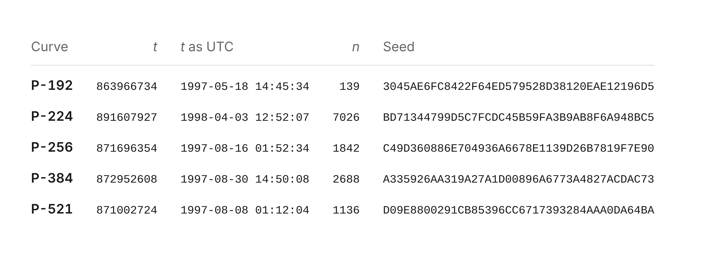
What this means

This is not a cryptographic break, new attack, or weakness in the ECDSA curves. In fact, this makes us more confident the curves were chosen without any backdoors or intentional weaknesses. For many years, people have been suspicious of the origins of the NIST curve parameters. They were presented to NIST without any mention of how they were chosen, leaving people wondering if they may have been chosen to have deliberate backdoors in them. These findings make that much less plausible. The seeds were generated in a very simple way: a common pseudorandom number generator initialized from the clock, which anyone can now reproduce. That leaves much less room for subversion and that we can be confident the parameters are secure.

How it was found

Searches for the phrase, built from the rumors, had come up empty. Claude tried a different angle: anticipating how the software that generated the curves must have worked. Claude guessed the software used a pseudorandom number generator (PRNG) that shipped with 1990s C libraries. These old PRNGs are weak enough that their output can be recognized. Recognizing that output would reveal which PRNG was used and possibly allow recovery of its initialization state.

Claude wrote a scanner that slid along each published seed one bit at a time and tested whether adjacent chunks were consecutive outputs of a 1990s-vintage generator. The scan covered 34 combinations of generator and output slices. At that point, Claude noticed a pattern in the top bits for some seeds: they were all zero. Written as five 32-bit words, four of the ten seeds have a 0 in the top bit for all 20 words. That would happen by chance with probability 1/5810. That was a signature of the linear congruential generator lrand48, which only returns the top 31 bits of a 48-bit state. The pattern is visible by eye once you know to look for it. To recover the state, Claude took the first word, tried all 2¹⁷ values of the 17 hidden bits, and checked that the next four words followed. That worked for all four seeds under discussion.
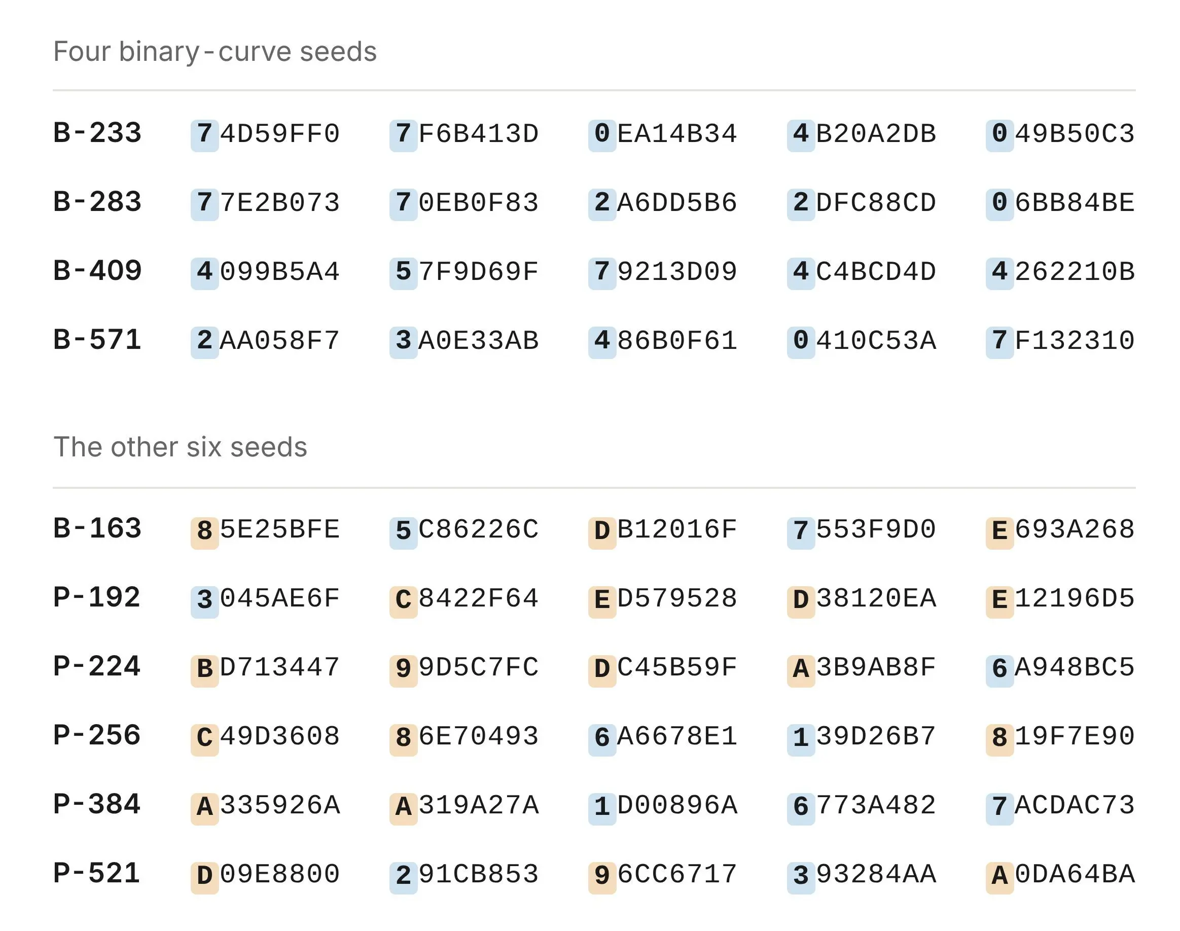
The prime-curve seeds came from the same lrand48 generator but kept fewer bits of each output. Claude had to recover the internal state of the PRNG from those bits. It turns out recovering the state of a truncated linear congruential generator is a textbook lattice problem, solved with the Lenstra–Lenstra–Lovász (LLL) basis reduction algorithm. Claude didn’t know which bits of the state the seeds might show, so it ran the solver over every window. Five NIST prime-curve seeds plus five more from the ANSI X9.62 standard all had the same pattern: lrand48() >> 23. Each recovered 48-bit state regenerates all 160 bits of its seed, which does not happen by chance.
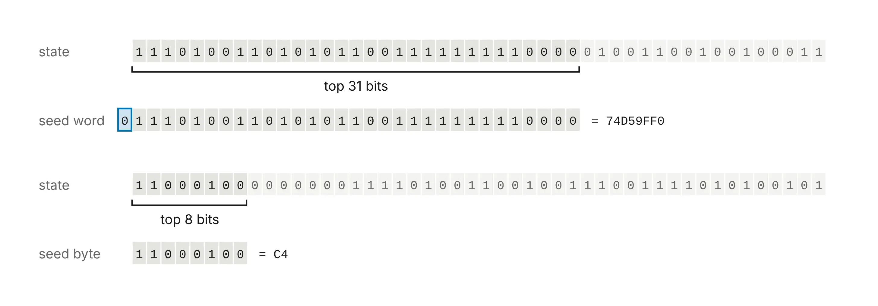
This linear congruential generator runs backwards as easily as forwards, so for each seed Claude stepped the state back until it reached the form that it would have been initialized by srand48, with the low 16 bits equal to 0x330E. The internal PRNG state of that form would come up once every 65,536 steps, so reaching one is not evidence on its own.

However, for the ten prime-curve seeds, every srand48 initialization was a Unix timestamp representing a date between May 1997 and April 1998. They were using the weak PRNG seeded by Unix timestamp. The four binary-curve initializations read as February 1984. With the timestamps doubled, they map to April 17, 1998, two weeks after the P-224 run. So, the program may have halved the clock.

Claude’s internal thinking at the time was:

This is astonishing: it solves the 25-year-old mystery. Hmm wait. Let me be skeptical: am I in some sort of simulated/test environment? … The seeds match my memory of actual values … Hmm, is it plausible in reality? As of my knowledge … the bounty was unsolved. … All top bits clear—20 bits, chance 1e-6. So indeed real-world. Wow, it's a real discovery.

Hmm wait. Let me be careful about the plausibility: is it suspicious that such an obvious thing wasn’t discovered in 25 years? It’s verified by direct computation on my side: 160-bit match from a 32-bit seed + small index: no chance coincidences (10 × 160 bits). It’s real.

Claude found some base points too

But wait, there’s more… Each curve also comes with a base point, G, the fixed point that every ECDSA public key is a multiple of. The seed found above does not determine this G, and so another question arises: how were these base points generated?

While checking the seeds, Claude also found where some of the base points came from. The base points of the six curves generated in May 1997 (P-192 and the five ANSI X9.62 example curves prime192v2, prime192v3 and prime239v1 to v3) come from the random number generator in FreeLIP, Arjen Lenstra's long-integer arithmetic package. Early versions of Victor Shoup's NTL library shipped the same code.

The recipe here is simple:

  1. Seed the generator with a small integer.
  2. Throw away seven outputs.
  3. Generate candidate x-coordinates from 26-bit outputs reduced mod p.
  4. Repeat step 3 until x is on the curve.

Claude found the generator seeds are 20000 for P-192, 20420, 20507 and 20509 for prime239v1 to v3, and 20512 and 20517 for prime192v2 and v3.
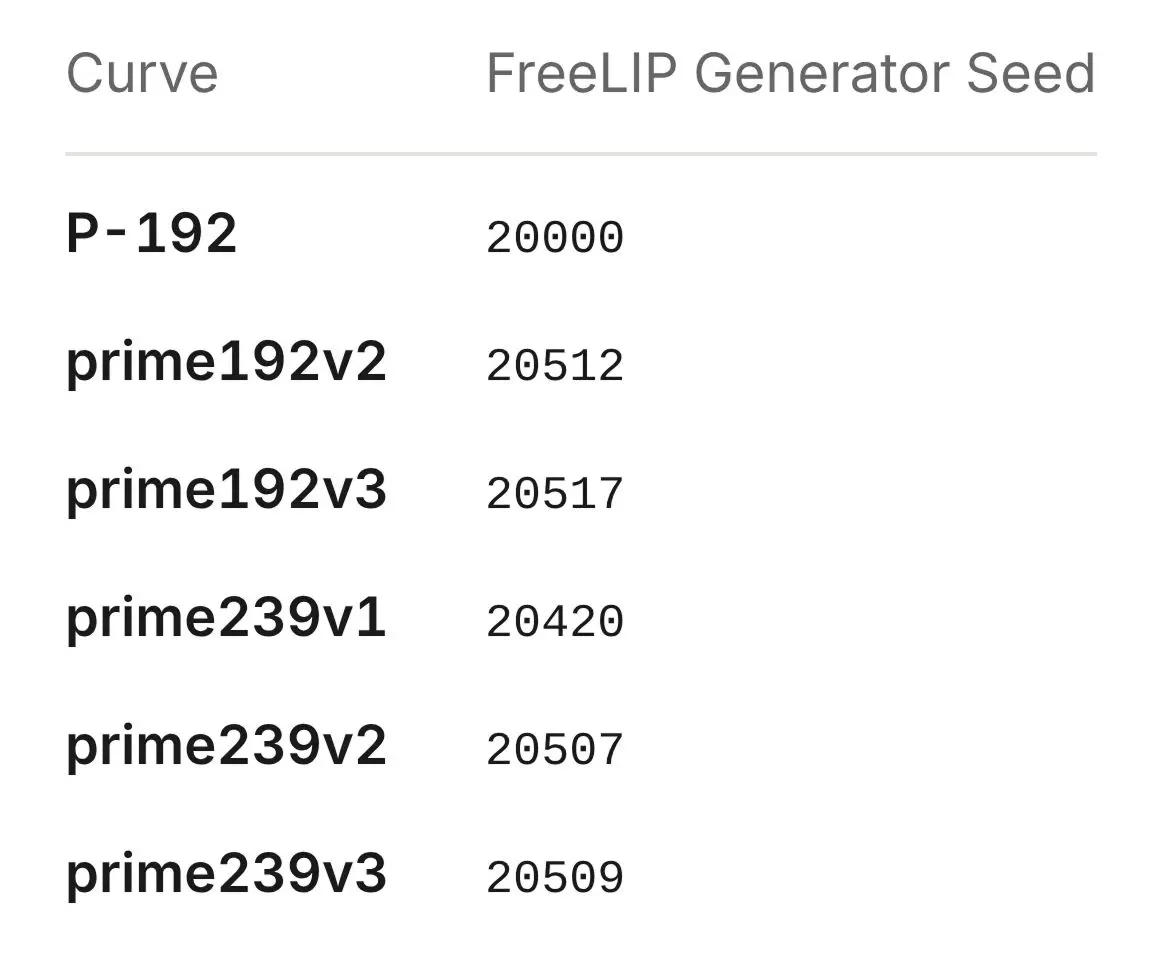
As far as we know, no NIST base point has been explained before. The base points of P-224, P-256, P-384 and P-521 don’t fit this recipe; we weren’t able to explain how they were selected.

Open questions

Not every 20-byte candidate seed could generate a viable curve and we observed that some potentially viable curves were skipped. For P-256, the published seed is candidate 1842, but candidate 876 of the same run also gives a prime-order curve of the right size and with parameters chosen the same way as on the published curve. P-224's run passed over three such curves, and the two runs behind the ANSI X9.62 example curves passed over seven more (see figure). We do not know what criteria may have been used, or whether this was an unintentional artifact.
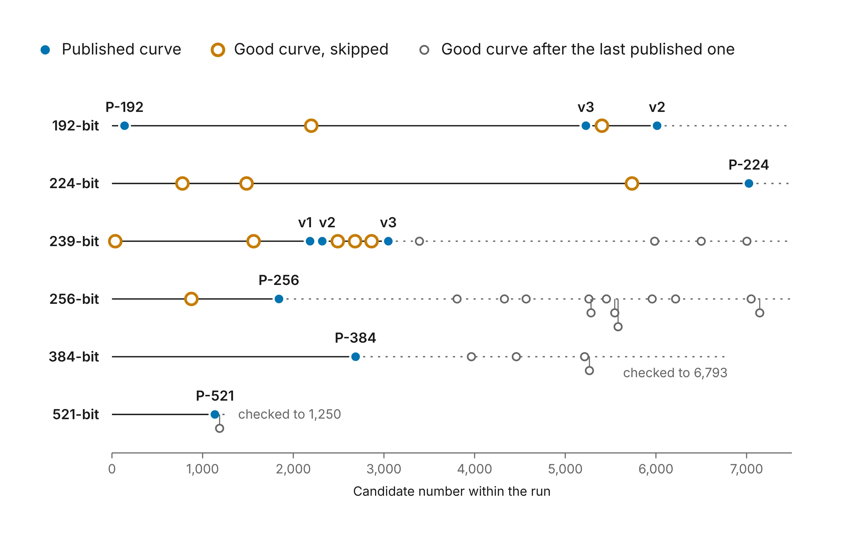
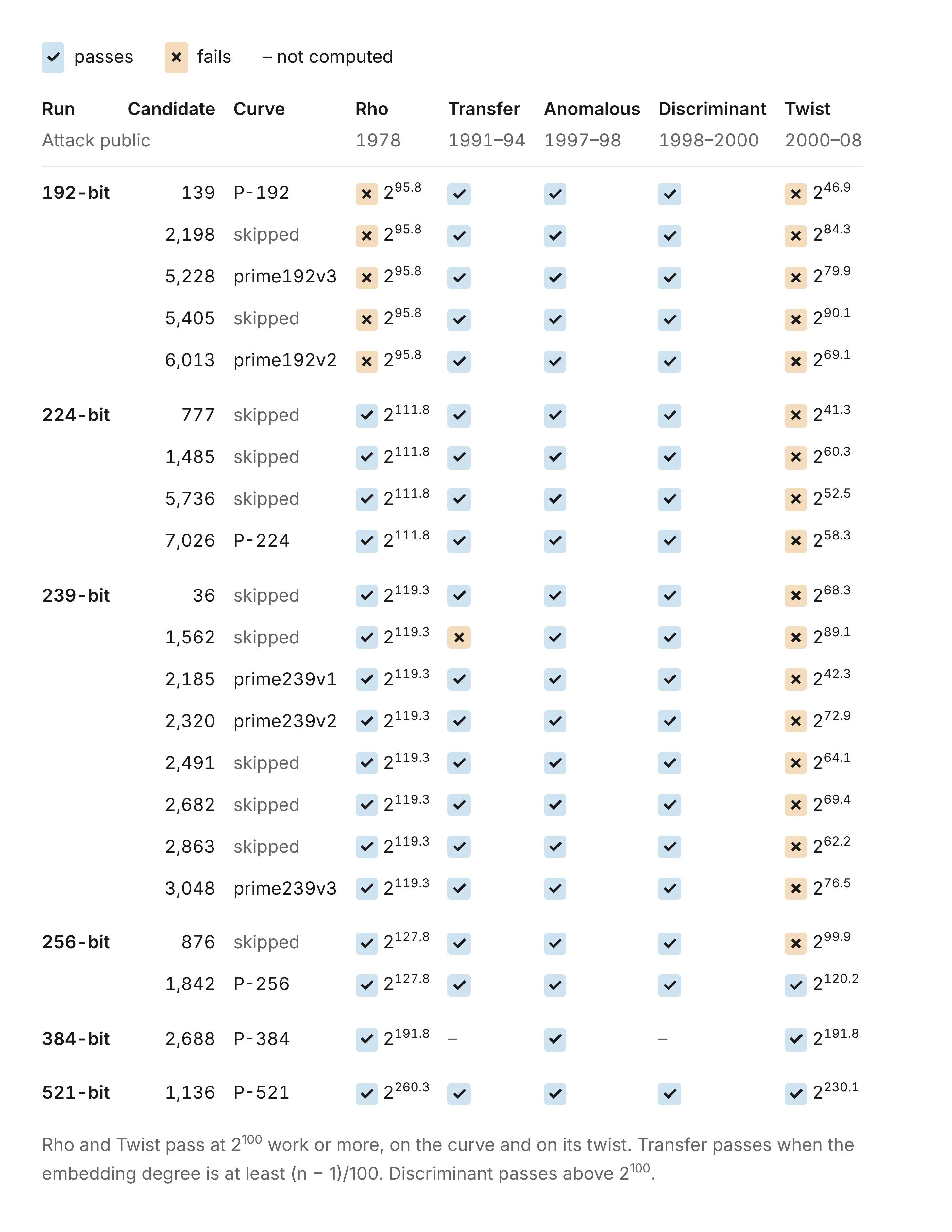
Because the number of skipped candidates is small, we do not believe it is plausible that weakened curves were selected. That would imply that weakened curves are common and easy to find. It is still conceivable that these curves were selected to have a specific property in principle by searching over timestamps to the random number generator. However, you would only need to do that if you were going to disclose the timestamp as some evidence that the seed was innocuously generated. Nothing in the numbers shows how many runs there were.

There is also one seed we were unable to recover. The fifth binary seed, B-163, fits nothing Claude has tried and remains unexplained. Finally, we don’t know how the base points for P-224, P-256, P-384, and P-521 were generated. The same goes for the NIST binary curves.

The bounty

The $36,864 for finding the seeds will be donated to the Internet Security Research Group.

Who we are

This work was conducted at Anthropic by John Wood, Henry de Valence, Ava Howell, Zack Voase, Lucy Sweet, Amir Omidi, Paul Crowley, Iain McGinniss, Nicholas Carlini, and Steve Weis.

Acknowledgements

We would like to posthumously recognize Jerry Solinas who took being labeled an “evil Internet meme” and the “Yo La Tengo of NSA bogeymen” with good humor. Also thanks to Filippo Valsorda for organizing the NIST Elliptic Curves Seeds Bounty.

Code to reproduce the seeds

from datetime import datetime, timezone

def unix(when):
    return int(datetime.fromisoformat(when).replace(tzinfo=timezone.utc).timestamp())

def candidate(t, n, per, shift, width):
    x, out = (t << 16) | 0x330E, ""                      # the state srand48(t) sets
    for i in range(per * n):
        x = (0x5DEECE66D * x + 0xB) % 2**48              # one step of lrand48
        if i >= per * (n - 1):
            out += "%0*X" % (width, x >> shift)
    return out

PRIME = {  # srand48(time); 20 bytes per candidate: lrand48() >> 23
    "prime239v1": ("1997-05-15 15:49:03", 2185),
    "prime239v2": ("1997-05-15 15:49:03", 2320),
    "prime239v3": ("1997-05-15 15:49:03", 3048),
    "P-192":      ("1997-05-18 14:45:34", 139),
    "prime192v3": ("1997-05-18 14:45:34", 5228),
    "prime192v2": ("1997-05-18 14:45:34", 6013),
    "P-521":      ("1997-08-08 01:12:04", 1136),
    "P-256":      ("1997-08-16 01:52:34", 1842),
    "P-384":      ("1997-08-30 14:50:08", 2688),
    "P-224":      ("1998-04-03 12:52:07", 7026),
}
BINARY = {  # srand48(time / 2), if that reading is right; 5 words per candidate: lrand48()
    "B-233": ("1998-04-17 15:24:18", 155),
    "B-283": ("1998-04-17 15:27:44", 32),
    "B-409": ("1998-04-17 15:30:18", 60),
    "B-571": ("1998-04-17 15:32:08", 73),
}
for name, (when, n) in PRIME.items():
    print(f"{name:10} {when} {n:5} {candidate(unix(when), n, 20, 40, 2)}")
for name, (when, n) in BINARY.items():
    print(f"{name:10} {when} {n:5} {candidate(unix(when) // 2, n, 5, 17, 8)}")

The output of this code:

prime239v1 1997-05-15 15:49:03  2185 E43BB460F0B80CC0C0B075798E948060F8321B7D
prime239v2 1997-05-15 15:49:03  2320 E8B4011604095303CA3B8099982BE09FCB9AE616
prime239v3 1997-05-15 15:49:03  3048 7D7374168FFE3471B60A857686A19475D3BFA2FF
P-192      1997-05-18 14:45:34   139 3045AE6FC8422F64ED579528D38120EAE12196D5
prime192v3 1997-05-18 14:45:34  5228 C469684435DEB378C4B65CA9591E2A5763059A2E
prime192v2 1997-05-18 14:45:34  6013 31A92EE2029FD10D901B113E990710F0D21AC6B6
P-521      1997-08-08 01:12:04  1136 D09E8800291CB85396CC6717393284AAA0DA64BA
P-256      1997-08-16 01:52:34  1842 C49D360886E704936A6678E1139D26B7819F7E90
P-384      1997-08-30 14:50:08  2688 A335926AA319A27A1D00896A6773A4827ACDAC73
P-224      1998-04-03 12:52:07  7026 BD71344799D5C7FCDC45B59FA3B9AB8F6A948BC5
B-233      1998-04-17 15:24:18   155 74D59FF07F6B413D0EA14B344B20A2DB049B50C3
B-283      1998-04-17 15:27:44    32 77E2B07370EB0F832A6DD5B62DFC88CD06BB84BE
B-409      1998-04-17 15:30:18    60 4099B5A457F9D69F79213D094C4BCD4D4262210B
B-571      1998-04-17 15:32:08    73 2AA058F73A0E33AB486B0F610410C53A7F132310

Code to reproduce selected base points

M, A = 2**107 - 1, pow(3, 121, 2**107 - 1)       # zrandom: state = state * 3^121 mod (2^107 - 1)
P192 = 2**192 - 2**64 - 1
P239 = 2**239 - 2**143 - 2**95 + 2**47 - 1

CURVES = [  # name, LIP seed, p, b, published Gx   (a = -3 throughout)
    ("prime192v1", 20000, P192,
     0x64210519e59c80e70fa7e9ab72243049feb8deecc146b9b1,
     0x188da80eb03090f67cbf20eb43a18800f4ff0afd82ff1012),
    ("prime239v1", 20420, P239,
     0x6b016c3bdcf18941d0d654921475ca71a9db2fb27d1d37796185c2942c0a,
     0xffa963cdca8816ccc33b8642bedf905c3d358573d3f27fbbd3b3cb9aaaf),
    ("prime239v2", 20507, P239,
     0x617fab6832576cbbfed50d99f0249c3fee58b94ba0038c7ae84c8c832f2c,
     0x38af09d98727705120c921bb5e9e26296a3cdcf2f35757a0eafd87b830e7),
    ("prime239v3", 20509, P239,
     0x255705fa2a306654b1f4cb03d6a750a30c250102d4988717d9ba15ab6d3e,
     0x6768ae8e18bb92cfcf005c949aa2c6d94853d0e660bbf854b1c9505fe95a),
    ("prime192v2", 20512, P192,
     0xcc22d6dfb95c6b25e49c0d6364a4e5980c393aa21668d953,
     0xeea2bae7e1497842f2de7769cfe9c989c072ad696f48034a),
    ("prime192v3", 20517, P192,
     0x22123dc2395a05caa7423daeccc94760a7d462256bd56916,
     0x7d29778100c65a1da1783716588dce2b8b4aee8e228f1896),
]

def base_point_x(seed, p, b):
    state = seed                         # zrstarts(seed)
    def limb():                          # zrandom(2^26): low 26 bits of the new state
        nonlocal state
        state = state * A % M
        return state % 2**26
    for _ in range(7):                   # seven single-limb draws come first
        limb()
    limbs = -(-p.bit_length() // 26) + 1 # zrandomb(p): limbs of p plus one, top limb first
    tries = 0
    while True:
        x = 0
        for _ in range(limbs):
            x = x << 26 | limb()
        x %= p
        tries += 1
        if pow(x**3 - 3*x + b, (p - 1) // 2, p) == 1:   # is x on the curve?
            return x, tries

for name, seed, p, b, gx in CURVES:
    x, tries = base_point_x(seed, p, b)
    print(f"{name:20} seed {seed}  tries {tries}  matches published Gx: {x == gx}")

The output of this code:

prime192v1           seed 20000  tries 2  matches published Gx: True
prime239v1           seed 20420  tries 3  matches published Gx: True
prime239v2           seed 20507  tries 2  matches published Gx: True
prime239v3           seed 20509  tries 1  matches published Gx: True
prime192v2           seed 20512  tries 5  matches published Gx: True
prime192v3           seed 20517  tries 1  matches published Gx: True

License

To the extent possible under law, the authors have waived all copyright and related or neighboring rights to the code on this page, dedicating it to the public domain under CC0 1.0 Universal (https://creativecommons.org/publicdomain/zero/1.0/).
The Daily Front Page 3 of 31
Friday, October 16, 2026 The Daily Front No. #261016 — The Work AI Has Yet to Measure
article

90% of US working hours are spent on tasks not covered well by AI benchmarks

by speckx·▲ 511 points·435 comments·mercor.com ↗
AI benchmarks have multiplied in recent years, but coverage of economically valuable work remains limited.

AI benchmarks have multiplied in recent years, but coverage of economically valuable work remains limited. To measure this, we compiled relevant benchmarks to measure their coverage of American jobs. This Benchmark Map is our first step toward building a comprehensive, continuously updated resource for understanding AI capabilities across the economy.

The Benchmark Map

Each tile represents one of the 923 O*NET occupations making up the US labor force, grouped into 22 job families. Occupations are shaded according to the share of their tasks which are represented in our initial list of AI benchmarks. A single benchmark prompt can be mapped to multiple O*NET tasks.

In our data set: only 208 of 923 occupations have a task with at least 5 benchmark prompts, and 6 of 22 job families have no such occupations.

Our findings suggest that 90% of American working hours are spent on tasks with little or no coverage from existing benchmarks. This makes it very hard to know how good AI models are at the work Americans actually do.

The coverage of existing benchmarks is not random, either. Our map suggests that the AI community is focusing on the largest labor markets first:

Each point shows the estimated probability that an O*NET task with a given AI-exposure tag belonging to an occupation with a given wage-bill will be covered by at least 5 prompts in our benchmark index. AI-exposure tags are binary and come from Eloundou et al. (2023). Occupation wage-bills are calculated from BLS estimates of the mean wage and number of Americans working in each occupation, assuming a 40 hour work week. Estimated coverage probabilities come from a task-level logistic regression of coverage probability on AI-exposure and log occupational wage bill. Error bars are pointwise 95% delta-method confidence intervals based on standard errors clustered at the occupation group level.


For example, benchmarks in our initial list heavily cover AI-exposed lawyers’ tasks, but barely cover any of the O*NET tasks of similarly AI-exposed legal secretaries or court clerks. The long tail of smaller, middle-income knowledge work jobs appears undercovered.

As we build out our coverage of model capabilities across the economy, we hope to both surface and help fill more gaps in our understanding of what models can do.

Methodology in brief

To break down the economy into sectors, occupations, and tasks, we used the US Department of Labor’s O*NET taxonomy. O*NET divides the US workforce into 923 occupations; for each occupation, O*NET attempts to provide a comprehensive list of “tasks” which make up the occupation, totaling 18,797 tasks across all occupations.

Example — 6 of the 22 tasks O*NET associates with Lawyers

  1. Prepare, draft, and review legal documents, such as wills, deeds, patent applications, mortgages, leases, and contracts.
  2. Advise clients concerning business transactions, claim liability, advisability of prosecuting or defending lawsuits, or legal rights and obligations.
  3. Interpret laws, rulings and regulations for individuals and businesses.
  4. Analyze the probable outcomes of cases, using knowledge of legal precedents.
  5. Present evidence to defend clients or prosecute defendants in criminal or civil litigation.
  6. Supervise legal assistants.

To measure benchmark coverage, we start with a list of 29 benchmarks selected for their quality and economic relevance. (The full list and selection criteria are in the Benchmark Index tab). In selecting benchmarks for this list, we prioritized:

  • Public Availability. Included benchmarks have at least 25 publicly available tasks. We also include Mercor’s APEX benchmarks, where we have access to held-out benchmark prompts and are therefore able to map them to O*NET tasks.
  • Agentic Tasks. Included benchmarks ask models to perform agentic tasks, rather than answering questions or advising the user on how to complete a task.
  • Economic Realism. Benchmark tasks resemble tasks which humans (or agents) are frequently asked to do in real-world enterprises. Economically valuable tasks are prioritized over academically complex ones.
  • Economic Diversity. We capped the number of included benchmarks per job family, in significant part to account for the massive overrepresentation of software engineering and research tasks in popular benchmarks.
  • Balanced Difficulty. Benchmarks are not yet saturated by frontier models.

Following work by Wang et al., we then ask an LLM judge to tag each benchmark prompt with as many O*NET tasks as it thinks correspond to that prompt. We validate our LLM tagging with human expert tags on Mercor’s APEX benchmarks, a subset of this list of 29. On the Benchmark Map, an O*NET task counts as “covered” if our LLM judge has mapped it to at least 5 prompts from our 29 benchmarks.

To estimate the total share of working hours Americans spend on tasks covered by benchmarks on this list, we combine our coverage estimates with Hatgis-Kessell et al.’s LLM-derived estimates of the working time share of each O*NET task.

A more detailed account of our methodology can be found in the Methodology tab.

Limitations

Our estimates of total economic coverage, and of patterns in coverage, all come from the initial list of 29 benchmarks we chose. This is not a complete or perfectly representative sample of the broader universe of unsaturated, public, agentic economic benchmarks. Any incomplete list will necessarily bias down estimates of economic coverage, and it is difficult to bound that bias. We want to stress, therefore, that these results are provisional. We will update them as we expand the initial benchmark list.

We also capped the number of included benchmarks in each job family in order to maximize breadth of coverage. We think this makes our estimate of economy-wide benchmark coverage more accurate, at the cost of biasing down our estimates of coverage in the most-benchmarked job families (e.g. software engineering).

By selecting for unsaturated benchmarks, we risk understating benchmark coverage on O*NET tasks which are easier for LLMs to complete. On the other hand, including saturated benchmarks would risk overstating benchmark coverage if saturation is downstream of lower task realism. The latter claim seems likely, given that benchmarks often overstate LLM performance in real-world deployments. We think that the bias from including saturated benchmarks would be greater than the bias from excluding them, but neither option is ideal.

Finally, while we outline our benchmark selection criteria in the Benchmark Index tab, several criteria (like “Economic Realism”) are difficult to formalize and introduce some subjectivity in our choices.

Patterns in coverage

The benchmarks in our index have relatively deep and narrow coverage of the overall economy. They disproportionately focus on the economic tasks most exposed to AI automation (as measured by Eloundou et al.), with O*NET tasks rated as “exposed” about 6x more likely to be represented on benchmarks than tasks rated “unexposed”. This makes sense: benchmarks are designed to measure AI progress, and AI progress is most plausible on the most AI-exposed tasks. This explains why benchmarks are full of tasks in Software Engineering and Financial Analysis while sparse on tasks in Truck Driving and Gas Plant Operation.

But even after controlling for AI-exposure, O*NET tasks from occupations with larger wage bills are significantly overrepresented among benchmark prompts:

Each point shows the estimated probability that an O*NET task with a given AI-exposure tag belonging to an occupation with a given wage-bill will be covered by at least 5 prompts in our benchmark index. AI-exposure tags are binary and come from Eloundou et al. (2023). Occupation wage-bills are calculated from BLS estimates of the mean wage and number of Americans working in each occupation, assuming a 40 hour work week. Estimated coverage probabilities come from a task-level logistic regression of coverage probability on AI-exposure and log occupational wage bill. Error bars are pointwise 95% delta-method confidence intervals based on standard errors clustered at the occupation group level.

After controlling for occupation and AI-exposure score, O*NET “task importance” is another predictor of benchmark coverage. In particular, O*NET tasks come with domain expert estimates of the importance of the task for its occupation on a scale of 1-5. We find that the tasks scored most important are about 6–10x more likely to be represented on benchmarks than those scored least important:

Each point shows the estimated probability that, controlling for occupation, an O*NET task with a given AI-exposure tag and a given quintile O*NET importance score is covered by at least 5 prompts in our benchmark index. AI-exposure tags are binary and come from Eloundou et al. (2023). Importance quintiles are calculated from O*NET importance scores. Estimated coverage probabilities come from a task-level logistic regression of coverage probability on AI-exposure and importance quintiles, with occupation fixed effects. Error bars are pointwise 95% delta-method confidence intervals based on standard errors clustered at the occupation group level.

The plots above suggest a reasonable allocation of the relatively limited resources devoted to high-quality, economically relevant benchmarks so far; it’s natural to prioritize making benchmarks which cover the most important and AI-exposed tasks in the occupations with the largest wage bills. But barring a significant increase in the number and diversity of such benchmarks, these patterns will result in significant blind spots in our view of economically valuable model capabilities.

Can O*NET + benchmarks tell us how good AI is at your job?

Measuring model capabilities by job occupation is essential – for enterprises deciding which models fit their needs, for policymakers forecasting the economic impact of AI, and for Americans thinking about their careers. Unfortunately, this is a hard problem to solve.

We could just try averaging model performance on all benchmark prompts relevant to a given job. But as our Benchmark Map suggests, benchmarks cover some economic tasks much more intensively than others. A simple average would give too much weight to frequently benchmarked tasks.

O*NET offers a way to potentially reduce this bias. If we average model performance on occupation-relevant benchmark prompts weighted by O*NET classification, so that each O*NET task is equally weighted in our occupation average, we get a step closer to a number that represents real economic performance.

As a first step, we try this approach on Mercor’s APEX benchmarks for four occupations: investment banking, law, accounting, and software engineering. We compare O*NET-weighted scores to simple averages of model performance on tasks related to each occupation. The resulting weighted and unweighted scores are generally quite similar:

For each occupation, we take all prompts across APEX benchmarks related to that occupation. Darker bars show a simple average of model scores on those prompts for each occupation. Then, we sort the prompts by O*NET task. For each O*NET task with at least 5 corresponding APEX prompts, we average model scores on those prompts to get a task-level score. Next, we average each task-level model score to get occupation-level scores which weight performance on each O*NET task equally. (If an O*NET task has fewer than 5 prompts, we drop it from the average). Lighter bars show these weighted scores for each occupation.

In this case, at least, O*NET weighting changes very little. Model performance on APEX prompts is similar across the O*NET tasks included in the weighted scores above, which limits the value of reweighting. However, less than ⅓ of the O*NET tasks relevant to the 4 occupations above have enough APEX coverage to be included in our weighted scores. We are hopeful that applying O*NET weighting to a much larger set of benchmarks will result in high-quality occupation-specific model scores, and are working toward that goal.

However, even if we incorporate tasks from dozens of benchmarks, several obstacles remain:

  1. How do we navigate low statistical power?

    The sheer breadth of work done in the US economy means that for any O*NET occupation and task, we have relatively few benchmark items. This means that our estimates are inherently underpowered, and just one or two low-quality items can severely bias our scores.

  2. How do we account for the varying difficulty and fidelity of tasks?

    Some benchmark items are highly saturated, whereas others are still unsolved. This is partly a function of time (as older benchmarks were designed for less performant models and simpler environments) and partly a function of quality (some benchmark items are simplistically graded, have minor mistakes, or can be reward hacked). We do not yet have an explicit way of weighting by quality.

  3. Can evals that primarily measure AI automation generalize to augmentation?

    In the real world, AI models are still primarily used by humans, rather than automating entire job functions end-to-end. Therefore, measuring the real-world occupation capabilities of a model should ideally include measuring how much the model augments human productivity. We have completed some early work in this direction, but finding a methodology that scales remains elusive.

  4. Can every O*NET occupation and task be measured with benchmarks?

    Knowledge-based work is well-suited to measurement through benchmarks because it is largely done on digital machines, like laptops and phones. Dingel and Neiman estimate that only 37% of US jobs could feasibly be done entirely from home, suggesting that ~63% of jobs involve some tasks with a physical-world component which would be hard to incorporate into current benchmarks. For now, this may not be a meaningful oversight – with the rapid development of robotics capabilities, we anticipate a significant need for physical task benchmarks.

We are actively working on these problems; if you are too, please reach out!

We are indebted to Wang et al. for the O*NET tagging methodology, and thank Nathan Lambert for feedback on a draft of this work.

The Daily Front Page 4 of 31
Friday, October 16, 2026 The Daily Front No. #261016 — Review by Machine
article

How the Claude Code team does code review

by pretext·▲ 358 points·332 comments·claude.dev ↗
We didn't remove review. But we did move most of the reading to machines.

We've said before that Claude writes about 90 percent of Claude Code's own code. So how do we review code at the volume we produce it? Does anyone read code anymore? And if something breaks, who catches it?

This post covers the code review flow on the Claude Code team and how it has evolved. From June to September, merged pull requests to Claude Code's codebase more than doubled while the share that had to be reverted fell by more than 40 percent.

We didn't remove review. But we did move most of the reading to machines, optimized for human time and attention, and invested heavily in making it fast and easy to undo mistakes.

RETHINKING THE PURPOSE OF CODE REVIEW

When agents write code, the number of changes goes up, fast. In Anthropic's monorepo, changes landing per day went from about 2,500 in May to more than 30,000 in September this year.

Claude Code lives in its own repository, separate from the monorepo, but it's seeing a lot of pressure too. When you are shipping this fast, manual, line-by-line code review is incredibly difficult if not impossible.

Code review does two jobs:

  1. Find and fix issues before they ship
  2. Build shared context and codebase understanding across the team

This article mainly focuses on finding and fixing issues, but we will come back to the second job near the end.

We think "did a human read the code?" is an imprecise proxy for "what could go wrong with this change, and which check—automated or human—is the right one to catch it?"

Asking that question also changed when review happens. Before, review was a gate at the end of the road: write the code, open a PR, wait for your colleague.

Now, review runs continuously, more like spellcheck while you write. Most changes have been reviewed and fixed by Claude at least once before a human is asked to look. This catches most routine mistakes, and saves team attention for higher-level questions and scrutiny.

THE SCARCE RESOURCE: HUMAN TIME AND ATTENTION

We want to preserve human time and attention for issues only humans can solve and make sure automated checks catch the rest. At our current rate of change, there is still an incredible amount of work for humans to do, and our team encounters new and novel challenges almost daily.

Human time covers both sides of review's cost: the time people spend reviewing, and the time they spend fixing what bad code breaks. Cutting the first doesn't help if the time just shows up in the second.

So the goal is that most pull requests in the Claude Code repos (the CLI, the desktop and web apps, and the mobile apps) merge with at most one human in the loop, who can be the author, with no increase in reverts or incidents. To measure human time, we track human approvals per PR (median and 95th percentile), human comments, and how long a PR waits on a person. Revert and incident rates are the guardrail: if they rise, we haven't saved human time, we've only moved it.

THE LIFE OF A CHANGE

A typical change, from an engineer's laptop (or a Claude session in Slack), goes through multiple layers of code review.

FIG A Most of the path is automated; a person's attention goes where the risk is

LAYER BY LAYER

FIG B Each layer catches some problems and misses others. Few get through all of them, and rollback handles the rest.

1. The work is verified before anyone else looks

Most review now happens before a PR exists. We give Claude something it can run—like tests, a build or a screenshot to compare against the design—and ask it to show the output instead of saying it's done. Then a subagent reviews the diff with fresh context. Both habits come from our best-practices guide.

Before opening a PR, many of us also run a few internal skills: one hunts for bugs, one simplifies the diff, and one checks the behavior end to end. UI changes also get checked against our design guidelines.

Boris Cherny, who created Claude Code, has called giving Claude a way to verify its work probably the most important thing for getting good results. He estimates it makes the final result two to three times better, and writes, "Verification looks different for each domain. It might be as simple as running a bash command, or running a test suite, or testing the app in a browser or phone simulator."

When the automated reviewer keeps flagging the same thing, we fix it at the source: in the skill, with a lint rule, or with updates to instructional files such as:

  • CLAUDE.md tells Claude what the project is: the stack, the conventions, the goals and the non-goals. Every review loads it, so in a large codebase we keep it short and point to other docs from there. The reviewer also flags code that breaks a convention in it, and changes that make a line in it out of date.
  • REVIEW.md, written by code owners, tells the reviewer what matters in their part of the code. We check separately whether the reviewer actually follows it. The good ones are short. They say what failure looks like in that repo (for docs it's "it lies," for config it's "it misroutes"), cap the nits, list paths to skip, and ask for a file and line as evidence instead of a guess from a name. They also ask for a summary that starts with a count and says plainly when there's nothing to fix.

2. AI review on every pull request

Every pull request gets a Claude review before a person looks. It reads the diff against the whole repo and the PR's stated intent, and asks: does the change solve its problem, fit the system, or break something else?

On a bug fix, it looks for the root cause. The public version, Code Review for Claude Code, is now generally available on Team and Enterprise plans, and /code-review runs a lighter version locally.

When we launched the research preview, the share of internal PRs getting substantive review comments went from 16% to 54%. Most PRs over 1,000 lines get findings, and most small ones come back clean. Admins set each repo to Quick, Standard, or Deep. Deep is worth it where one missed bug costs more than the extra review time.

Findings get verified by other agents before humans review them. Several agents look for bugs at the same time. Then a separate group votes on each finding, and it only gets posted if enough of them agree it's real. Findings that are only about style, diagnostics, or cleanup get dropped. We A/B tested those filters on our own PRs before keeping them. What's left shows up as inline comments sorted by severity. Each is tagged Important, Nit, or Pre-existing, so a bug the PR didn't introduce doesn't look like the author's fault.

Every finding has to be answered. You either fix it or resolve the thread with a reason. Often an agent picks up the fix overnight, so the author comes back to a PR that's already been through another round.

3. Security review that can block

Security gets its own automated review too. A PR can't merge while any finding from the bug review or the security review is still open. You either fix it or close the thread with a short reason, which is how you clear a false positive.

If a later commit fixes the issue, the finding clears on its own. You can set up the same thing with the open-source security review GitHub Action or the /security-review command. Setup is covered in automated security reviews in Claude Code.

4. Automated checks that block

The usual: lint, type checks, tests on every platform, and a build. (We wrote about scaling CI for this volume here.) A typical CLI pull request may run dozens of checks before anyone looks at it. The PR template asks how the change was tested and how to undo it. Claude can fill that in, but the person who asked for the change signs off on it.

5. Human approval, scaled by risk

A docs fix and an auto-updater change carry different risk, so they get different review.

Risk Examples Human approvals
Low Docs, copy, internal-only features, additive changes behind a flag None required once automated review and security checks are green
Medium Ordinary product changes, and changes to sensitive areas such as caching, the auto-updater, or system prompts One person
High The highest-risk code, plus a small set of paths that always need two people Two people

The change sets the tier, not the author. A classifier reads the change and picks its risk tier. A second classifier asks whether this particular change needs another person even when its tier says it doesn't. Some paths always need a person, anything owners have listed as sensitive and any CI workflow file.

Only trusted authors get the lighter paths. Only authors on the repo's trusted list get the lighter paths, mostly the team that owns it. Everyone else needs a second person to approve. An agent's approval never counts as a person's, either. Automated review can clear a low-risk change, but it can't fill a slot that calls for a human.

Whoever prompted the change is on the hook for it. On an agent-written PR, the person directing the agent counts as one of the required reviewers, the same as if they'd typed the code themselves.

An approval covers one specific commit. If new commits land that the system can't vouch for, like an agent's push or a merge someone resolved by hand, the approval has to be given again.

6. Merge queue, flags and a gradual release

The merge queue re-runs every check against main with the change applied, so two PRs that pass separately can't combine into a broken main. New behavior usually ships behind a flag to Anthropic employees first, and our heavy use often surfaces regressions before users do. Public releases go to the latest channel first. The stable channel trails it.

7. Fast detection, fast rollback

Some mistakes will still get through, so the last layer is about catching them fast. Flags turn off without a deploy. Claude Code has a weekly on-call rotation, and incident reviews ask which layer should have caught the issue.

Noticing a bad merge still depends on the author and on-call as well as the revert and incident dashboards. We don't yet have circuit breakers that tighten approval when those numbers move; engineers here want them before more code moves to zero-human merges.

One colleague said slowing down does lower your error rate, but mostly because you're doing less of everything. We'd rather get faster at noticing and fixing problems.

HOW WE MAKE THE REVIEWER BETTER

Our code review process is constantly improving in a loop.

Any incidents are now an eval. The team collected past PRs that caused incidents, with their fix-forwards and reverts, and had engineers who know that code confirm each bug and where it lived. The reviewer runs against that set daily.

FIG C The eval grows with every incident, and every change to the reviewer is scored against all of it.

We measure noise by watching what people do with the comments. It's easy to catch more bugs if you don't mind flagging a lot of non-bugs, so we need a check on that. We sort every comment the reviewer leaves by how the person on the PR responded: they fixed it, said it was wrong, said the behavior was intentional, or decided it didn't matter. We also run the reviewer on PRs we know are clean and count how often it reports something that would have led someone to make a harmful change. Our priority, written down, is catching real bugs first and cutting review rounds second.

Noise costs more when the author is an agent. A person can wave off a nit in seconds. An agent fixes it, which means another commit and another round of review.

Review has to converge. An agent author and an agent reviewer can keep each other busy indefinitely. One CLI PR went through more than fifty rounds of review and fixes overnight before its author stopped it.

When we ran git blame on what the reviewer kept flagging, about 59% of it was code that had been there since the reviewer's first pass. The reviewer was rarely finding new bugs, it was finding a few more old ones each round.

We made it worse ourselves. We'd gotten used to running several rounds by default, since each pass catches something new. This can be worthwhile on a risky change, but not on every PR. The team now tracks rounds-to-pass alongside recall, and changed re-review:

  • A round cap. After three rounds, the reviewer asks the author to step back and reconsider the approach.
  • Diff-only re-review after the first few passes.
  • Flag the class of bug, so the author fixes every instance, not one line.
  • No repeats of findings already posted.

Review agents also run nightly over existing code, helping us catch old bugs before they show up somewhere else.

FIG D Fewer review rounds per internal pull request after the convergence changes

WHERE HUMANS STAY IN THE LOOP

Pulling a senior engineer out of deep work to catch a routine mistake costs far more than an automated review. At Anthropic, our jobs have moved from reading every diff to the decisions machines are bad at:

  • Should we build this at all? Direction, taste and scope. One team that declared its review bottleneck solved still kept human review for changes from outside the team, so someone asks "should we even do this?"
  • Risky code such as billing, the auto-updater and CI workflows.
  • Architecture that sets a pattern others will copy.
  • Reading the evidence. Test output, the command that ran and what it returned, a screenshot, the reviewer's findings. If you can't say what the checks would miss, ask for a real review rather than a quick approval.
  • Owning the outcome. A person is accountable for every change that ships, whoever typed it.

FIG E People moved from reading every diff to the decisions machines are bad at

SHARING CONTEXT ACROSS THE TEAM

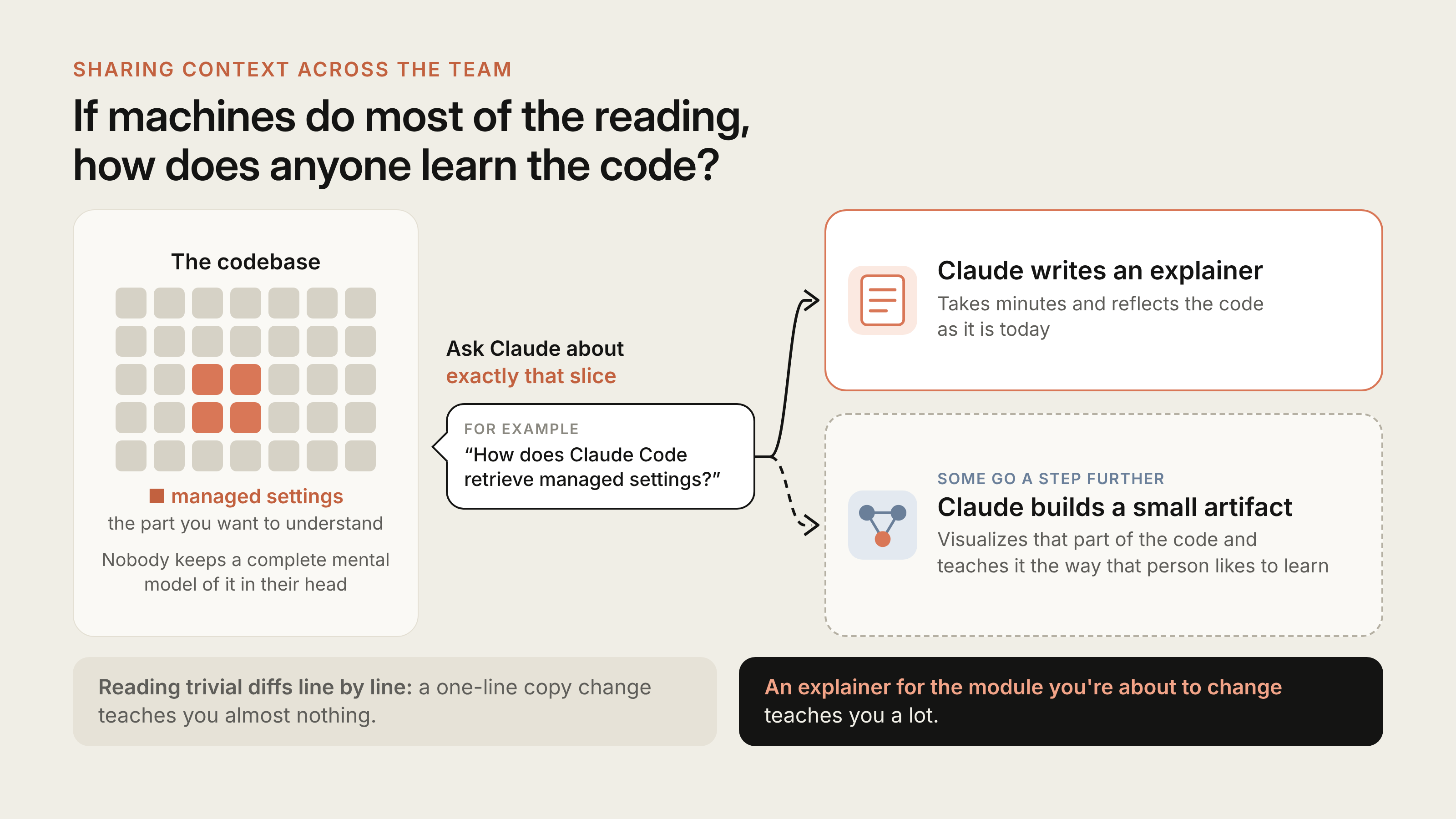
Code review's second job has always been to spread codebase understanding. Reading a teammate's diff is how you learn what changed and how the pieces fit. If machines do most of the reading, how does anyone learn the code?

We don't have a formal process for this. Nobody on the team keeps a complete mental model of Claude Code in their head, and we don't think anyone needs to. When someone wants to understand a part of the codebase, they ask Claude to write an explainer for exactly that slice. It takes minutes and reflects the code as it is today.

Diagram titled "If machines do most of the reading, how does anyone learn the code?" On the left, a grid stands for the codebase, with a few squares highlighted as managed settings, the part you want to understand; nobody keeps a complete mental model of it in their head. An arrow labeled "Ask Claude about exactly that slice", with the example question "How does Claude Code retrieve managed settings?", leads to two outcomes: Claude writes an explainer, which takes minutes and reflects the code as it is today; and, for some, Claude builds a small artifact that visualizes that part of the code and teaches it the way that person likes to learn. Along the bottom: reading trivial diffs line by line, a one-line copy change teaches you almost nothing; an explainer for the module you are about to change teaches you a lot.

Some of us go a step further and have Claude build a small artifact that visualizes that part of the code and teaches it the way that person likes to learn.

If the goal is to spend human attention well, this beats reading trivial diffs line by line. A one-line copy change teaches you almost nothing. An explainer for the module you're about to change teaches you a lot. Our culture of defaulting to working on open Slack channels helps too, since you see what others are building while they build it.

"YOU LAND IT, YOU OWN IT"

If you land a small or medium change and something still goes wrong, it's a team norm that you usually fix it. A few things keep this from going badly:

  • Changes are small, so they're easy to review, debug and revert.
  • Everything is reversible. Flags, reverts and staged releases undo most mistakes in minutes.
  • Blast radius sets the bar. Expensive code gets more people and more checks.
  • Regressions surface fast through telemetry and internal use.
  • It isn't blame. Owning a fix means you have the most context; incident reviews look at the system.

Ownership is also shared. Much of the team works in open channels where anyone can see what others are building, pick up a thread, or point a Claude at a gap, and feedback comes from people who don't own the code too. That openness is a big part of how quality stays high without a gate on every line.

WHEN WE CHANGE DIRECTION

Agents make it cheap to start things, so some work shouldn't land. Usually someone in the channel asks why, points at an earlier decision, or suggests a simpler route, and the author closes or reshapes the PR.

Since the code was fast to write, closing the PR doesn't feel like a loss. The trick is to raise a different direction in the thread early, not as a blocking comment on a finished PR.

HOW YOU CAN ADOPT THIS PROCESS

Most of the pieces to do this with your team exist today.

Before the pull request

  • Give your agent checks it can run, listed in a short CLAUDE.md, plus hooks that run formatters and linters.
  • Run /code-review and /security-review locally, or a fresh-context subagent review.
  • Add a REVIEW.md, and move repeated review comments into it.

On every pull request

  • Require CI, and add "Testing", "Risk" and "How to revert" to your PR template.
  • Add an AI reviewer (Code Review for Claude Code, or the Claude Code GitHub Action) on one repo, tune REVIEW.md for a few weeks, then widen.
  • Add automated security review, and require every review thread resolved before merge.
  • Match review effort to risk: a quick pass on routine changes, a deep one where a missed bug is expensive (Quick, Standard or Deep in Code Review).
  • Cap review rounds; after the first few, re-review only the new diff.

Approval

  • Write down risk tiers, set from the change rather than the author; start strict and loosen with evidence.
  • Keep the lighter approval paths for authors you trust.
  • Use CODEOWNERS and branch protection so auth, billing, CI and release workflows, and installers always need a person.
  • Never let a bot's approval replace a required human's; dismiss approvals on new commits.

Merge and after

  • Use a merge queue, feature flags, internal use first, staged releases and one-step rollback.
  • Turn incidents and reverts into an eval set, and rescore the reviewer whenever its prompts, tools or model change.
  • Measure human time, with revert and incident rates as the guardrail.

WHERE THIS IS GOING

Code Review's announcement said approving a pull request is still a human call; the product posts findings, not approvals. Our own repos go further, letting owners decide which low-risk changes merge on automated checks alone, and that line keeps moving.

When a review misses something, we ask what the model didn't have in front of it and put the fix into a CLAUDE.md, a skill or a new check. The goal hasn't changed: less human time per change, and no more reverts than before.

If your team lets agents open pull requests, we'd like to hear which checks you've automated, which still need a person, and what you think we have wrong.

With thanks to Emma Webb, Michael Segner and Amie Rotherham for their reviews.

The Daily Front Page 5 of 31
Friday, October 16, 2026 The Daily Front No. #261016 — Pixels by Hand
article

I love software rendering

by speckx·▲ 326 points·205 comments·jamesfmackenzie.com ↗
I love software rendering.

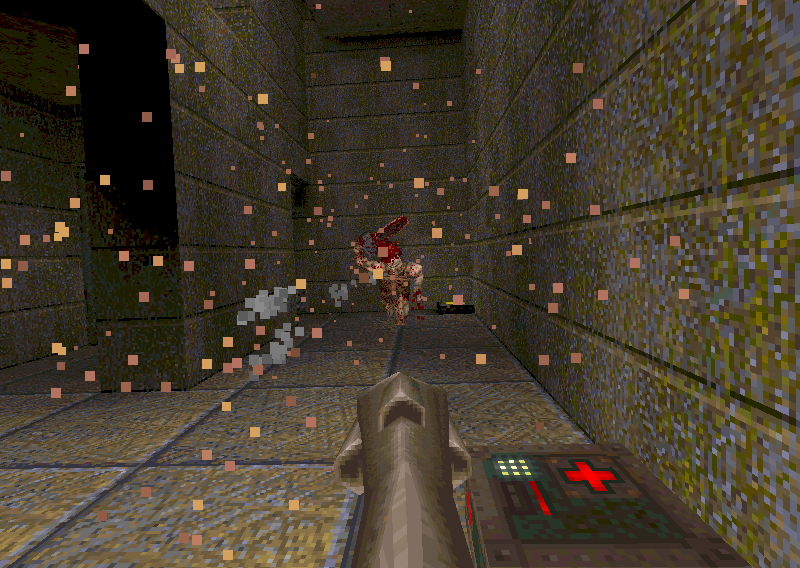
An ogre caught by a rocket in a Quake corridor, square particles flying through the air

Quake in its DOS software renderer, where even the particles are square. All the screenshots in this post are my own captures.

I love software rendering. The best DOS experience I’ve had in a long while was Quake in its software renderer at 800×600, running at a locked 60fps on my Dell OptiPlex 380. It’s one of the best-looking things I’ve seen a DOS game do.

That’s not how most people remember those games looking. In the 90s you either ran them in software at a low resolution, or you bought a 3D card and played the accelerated version. Today there’s a third option: run the software renderer on a machine fast enough to push it at resolutions nobody could use back then.

What software rendering is

In a software-rendered game, the CPU draws every pixel. There’s no 3D card involved: the game works out each frame in its own code and writes it straight to video memory. Doom, Duke Nukem 3D, Blood and the original Quake all work this way.

When 3D cards arrived, many games got accelerated versions. GLQuake came after Quake, and Blood and Tomb Raider got 3dfx modes. Those versions hand the drawing to the graphics card, and they look different.

Why I like the look

It’s sharp. Software renderers generally sample textures pixel by pixel, so every texel stays a crisp square. Early 3D cards smoothed textures with bilinear filtering, which looked impressive in 1997 but turns everything soft and blurry to my eye now.

A Quake rune on a wall, every texel a crisp square

It’s gritty. Most of these games ran in 256 colours, with lighting done through lookup tables into that palette. Shadows fall off in visible steps rather than smooth gradients. Technically that’s colour banding, a limitation. In practice it gives the games a rough, grimy texture that I really like, and that hardware rendering smooths away.

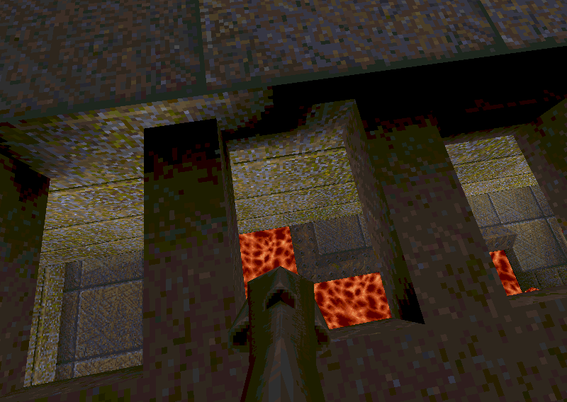
Lava glowing through openings in a grimy stone wall in Quake

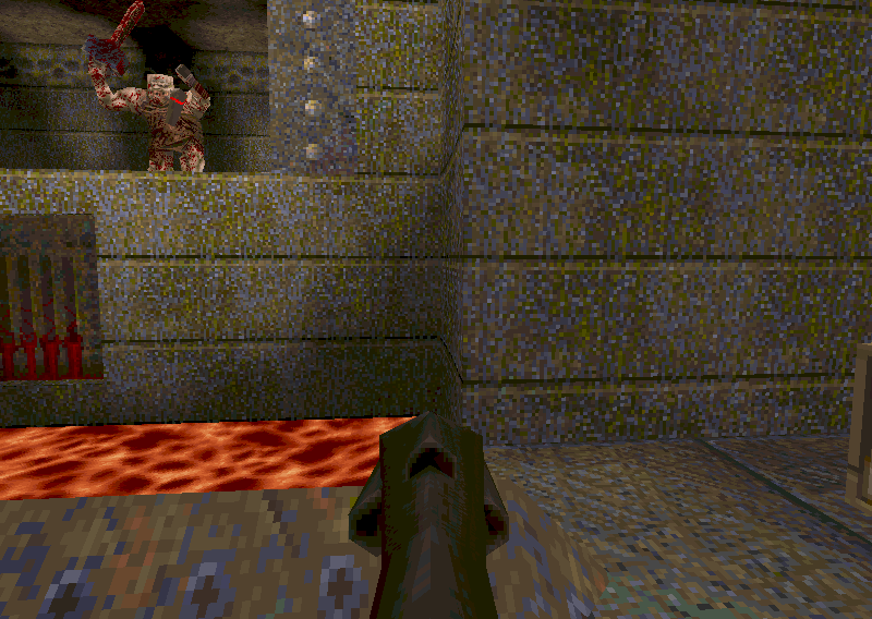
An ogre with a chainsaw on a ledge above a lava pool in Quake

It’s how the games were built. Quake was released with its software renderer, and GLQuake followed. Doom and the Build engine games were designed around their software renderers from the start.

It isn’t always the better option. When I got a Voodoo 2 running in a modern PC, Blood ran fast in its 3dfx mode, but the VESA software modes were the better-looking option. Tomb Raider went the other way: its underwater sections look noticeably better accelerated than in the DOS software renderer. So it’s a preference, not a rule. But for most of the games I care about, I’d pick the software renderer.

It’s not just nostalgia, either. Ion Fury, a Build engine game from 2019, still ships with a software renderer.

The catch: it needs a fast PC

Software rendering scales with the CPU. Every extra pixel is work for the processor, so the high VESA resolutions that many late DOS games offered were well beyond the hardware of the day.

Modern hardware can power through most of it. On the OptiPlex 380, Quake at 800×600 holds a locked 60fps. But the heaviest games still push even very fast machines. In his video on the Portwell RUBY-9719, Rasteri shows Build engine games needing far more power at high resolutions, to the point where even a 3.3GHz quad-core Xeon “isn’t quite enough to run Shadow Warrior at full 1600 by 1200”.

So if you want to see these games at their best, you want the fastest machine you can get that still runs them.

Why it needs native DOS

There are other ways to get software rendering on a modern PC. Source ports of Doom and Quake run software renderers on Windows, and Ion Fury runs on Windows natively. They’re great.

What I’m after is the original DOS versions running as they were released, on real hardware. DOSBox is the obvious alternative, but some DOS titles struggle in DOSBox, while on real hardware they behave exactly as intended.

That leaves one more problem: sound. A fast machine running native DOS needs a sound card the games can talk to, and modern PCs don’t have one. That’s a story of its own.

Games worth trying

  • Quake, in software at 800×600 or higher
  • Duke Nukem 3D and Blood, the Build engine games, at high VESA resolutions
  • Screamer

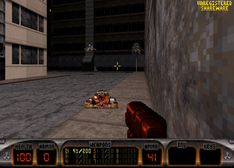
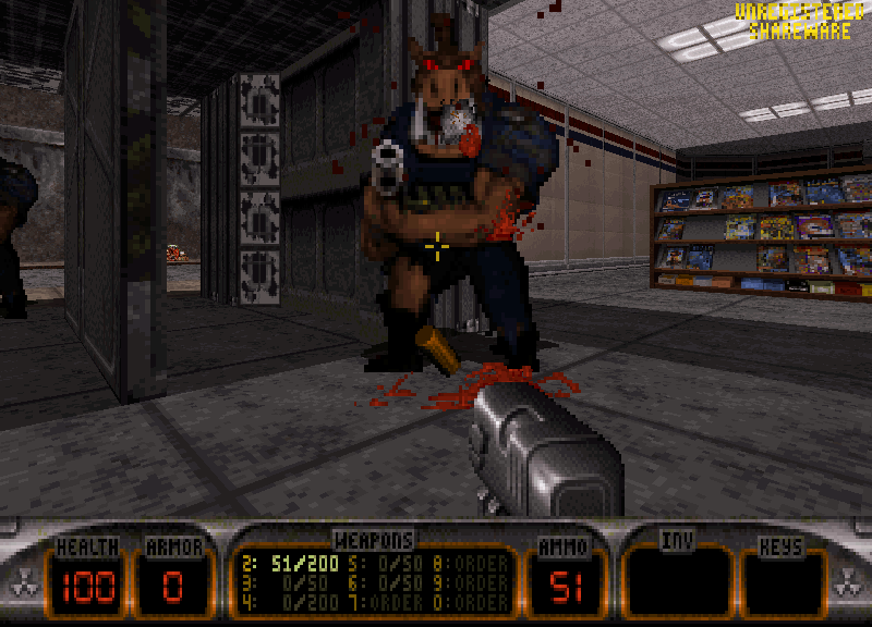
A city street in Duke Nukem 3D's first level A Pig Cop in a store in Duke Nukem 3D

The Daily Front Page 6 of 31
Friday, October 16, 2026 The Daily Front No. #261016 — The Desk-Sized Supercomputer
article

Apple ML Research: Muse Spark Open with MLX on Mac Studio

by antipaul·▲ 323 points·161 comments·machinelearning.apple.com ↗
enabling anyone to run new inference and fine-tuning methods on their own hardware

The MLX logo

MLX on Mac with Apple silicon lets AI researchers and developers experiment locally with the latest models and methods in a private environment. The open-source array framework leverages the unified memory architecture of Apple silicon, enabling anyone to run new inference and fine-tuning methods on their own hardware and explore other AI techniques. In a previous post, we highlighted the advantages of the M5 architecture and its GPU Neural Accelerators.

In this post, we show how to run the latest frontier-class model — Muse Spark Open, with nearly a trillion parameters — right from your desk, using the latest version of MLX, released today. On a cluster of four Mac Studios, Muse Spark Open generates over 36 tokens per second (see Figure 1), well above average human reading speed.

Beginning on a single Mac Studio (up to 512GB of unified memory), then scaling out across multiple Macs with the RDMA over Thunderbolt driver, below we share an overview of the range of models you can now run on Mac Studio.

Figure 1: Muse Spark Open decode speed in tokens per second, on Mac Studio with M5 Ultra, at a context size of 8,192 tokens. Higher is better. We report performance for three parallelization schemes: pipeline parallelization over two Mac Studio computers (2 M5 Pipeline), and tensor parallelization over two (2 M5 Tensor) and four Mac Studio (4 M5 Tensor) computers.

Running Large Language Models with MLX

We benchmark several popular open-weight LLMs on Mac Studio, using the MLX LM package, as described in our prior post. We compare two generations of Mac Studio: the recently released M5 Ultra and the previous generation, M3 Ultra. The M5 generation features the GPU Neural Accelerator, which supports dedicated matrix multiplication operations, essential for many machine learning workloads.

We evaluate three frontier-class models (Table 1) spanning a wide range of sizes (in billions of parameters, B): the newly released Muse Spark Open (816 B), Mistral Medium 3.5 (128 B), and Qwen 3.8 (27 B). Muse Spark Open is a mixture of experts (MoE) model, which keeps only a fraction of its experts — and thus parameters — active, reducing compute at inference, and it is evaluated in NVFP4 precision. Mistral Medium 3.5 and Qwen 3.8 are dense architectures, where all parameters are active at inference, and they are evaluated in their native floating-point precision (FP8 and BF16, respectively).

Model Total Parameters Active Parameters Native Precision Evaluation Precision
Muse Spark Open 816B 42B BF16 NVFP4
Mistral Medium 3.5 128B 128B FP8 FP8
Qwen 3.8 27B 27B BF16 BF16

Table 1: Language models used in this post. Models ship in various precision formats; we evaluate Qwen 3.8 and Mistral Medium 3.5 in their native precision, and Muse Spark Open in 4-bit (NVFP4) precision.

Our evaluation measures three metrics across a range of context sizes: time to first token (TTFT, in seconds), generation throughput (in tokens/second), and peak power usage (in watts). All the performance numbers in this post were obtained with mlx_lm.benchmark. For example, running Qwen 3.8 with 8,192 tokens of context and generating 128 tokens is performed with the command line:

mlx_lm.benchmark --model Qwen/Qwen3.8-27B -p 8192 -g 128 -b 1

A popular use of local LLMs on Mac Studio is running agentic experiences in a private environment, including agentic coding applications that often need large contexts. We therefore report performance at both 8,192 and 65,536 context sizes.

Raw TTFT and decode throughput are reported in Table 2 and Table 3, respectively.

Inference Performance on a Single Mac Studio

Qwen 3.8 27B and Mistral Medium 3.5 128B fit comfortably on a single Mac Studio with 512GB, taking up to 68GB and 158GB of RAM in the large context size (65,536 tokens) setup. In Figure 2, we compare their inference performance on a single Mac Studio with 512GB of RAM, both on M3 Ultra and M5 Ultra.

Time to first token (TTFT) is essentially compute bound, and that is where the Neural Accelerators in the M5 Ultra GPU shine: the specialized hardware support for fast matrix-multiplication of the GPU Neural Accelerator directly translates into significant speedups for TTFT, up to 4.6× faster compared to an M3 Ultra (see Figure 2). That makes the Mac Studio with M5 Ultra the desktop of choice when it comes to handling tasks involving very large contexts.

Generation speed (in tokens per second) is memory-bandwidth bound. The M5 Ultra chip delivers 1.2 TB/s of unified memory bandwidth, up from 819 GB/s for the M3 Ultra. Here again, that translates directly into generation speed (see Figure 3), with the Mac Studio with M5 Ultra reporting 1.6× faster tokens/s.

Figure 2: Time to first token (TTFT) speedup on M5 Ultra over an M3 Ultra baseline, for Qwen 3.8 and Mistral Medium 3.5, at context sizes of 8,192 and 65,536 tokens. The M5 Ultra GPU Neural Accelerator shines on compute-bound workloads.

Figure 3: Decode speedup on M5 Ultra over an M3 Ultra baseline, for Qwen 3.8 and Mistral Medium 3.5, at context sizes of 8,192 and 65,536 tokens. Decode is memory-bandwidth bound, and the M5 Ultra’s 1.2 TB/s of unified memory bandwidth (vs 819 GB/s on the M3 Ultra) is a key advantage.

The Mac Studio is also energy-efficient for LLM inference (see Figure 4): peak power consumption is about 200W for the Mac Studio with M3 Ultra, and 300W for the Mac Studio with M5 Ultra — a fraction of the power used by a common toaster. More importantly, that modest amount of power consumption means a Mac Studio can be deployed for AI work in any home or office environment.

Figure 4: Peak power consumption (in watts) during Qwen 3.8 and Mistral Medium 3.5 inference, at a context size of 65,536 tokens, on Mac Studio with M3 Ultra and with M5 Ultra.

While both the Qwen and Mistral models fit on a single Mac Studio with 512GB of RAM, Muse Spark Open would require more than 1.6TB of RAM in its native precision (BF16) for the model parameters alone. In a 4-bit quantized (NVFP4) format, the model memory footprint is lowered to about 493GB. Add the memory needed for intermediate computations during inference, and the model cannot fit on a single machine. It requires parallelization across multiple Mac Studio computers.

Pipelining Inference Across Two Mac Studio Computers

Very large frontier-class models like Muse Spark Open will not fit on a single machine. It is, however, possible to store half of the model on one Mac Studio and the other half on another. We can then pipeline the model’s inference across two computers: the first Mac Studio executes the first half of the model’s layers, then sends the output to the second Mac Studio, which executes the second half. This parallelization scheme is called pipeline parallelization (see Figure 5) and is extremely simple to implement, requiring only minimal code changes.

Figure 5: MLX supports two approaches to splitting large models across multiple computers. With pipeline parallelization, a model is split across depth, while with tensor parallelization, a model is split across width.

MLX supports different parallelization schemes, as described in the MLX distributed documentation. These rely on fast inter-machine communication: macOS 26.2 introduced a low-latency RDMA driver over Thunderbolt 5, and MLX (v0.30.1 and later) builds on top of this driver and provides new communication collectives (jaccl, pronounced “jackal”) for different parallelization schemes. In our setup, the two Mac Studios are connected with two Thunderbolt cables (to double the link bandwidth), providing the RDMA-over-Thunderbolt link that jaccl uses. Once the hosts are set up, MLX provides mlx.launch, a helper command to launch jobs across multiple nodes:

mlx.launch --hostfile hostfile.json --backend jaccl --env MLX_METAL_FAST_SYNCH=1 -- \
mlx_lm.benchmark --model mistralai/Mistral-Medium-3.5-128B -p 8192 -g 128 -b 1 --prefill-step-size 8192 --pipeline

In this command, --backend jaccl specifies the RDMA Thunderbolt driver backend. The --env MLX_METAL_FAST_SYNCH=1 flag enables an experimental MLX feature for fast CPU-GPU synchronization, reducing communication overhead between the CPU (which initiates the Thunderbolt communication) and the GPU (which does the compute).

In general, decode inference speed with pipeline parallelization (see Figure 7) is very similar to that of a single machine, since the layers are still evaluated sequentially. Communication overhead is also very low, as only the intermediate outputs between the two sets of layers need to be exchanged.

It is however notable that for very large contexts (65,536 tokens in our benchmark), pipeline parallelization ends up faster than a single node for prefill — up to ~1.8× faster (see Figure 6). This is because MLX segments large contexts into smaller chunks (here, 8,192 tokens, as set by --prefill-step-size 8192) and pipelines the prefill across the machines: while the second machine computes the later layers of chunk kkk, the first machine computes the earlier layers of chunk k+1k+1k+1, so consecutive chunks overlap in time. For even better compute parallelization, we next turn to tensor parallelization.

Figure 6: Time to first token (TTFT) speedup of two M5 Ultras with pipeline parallelization over a single M5 Ultra baseline, for Qwen 3.8 and Mistral Medium 3.5, at context sizes of 8,192 and 65,536 tokens. Splitting the context (here into 8,192-token chunks) lets MLX overlap computation across the two machines — hence the speedup at 65,536 but not 8,192.

Figure 7: Decode speedup of two M5 Ultras with pipeline parallelization over a single M5 Ultra baseline, for Qwen 3.8 and Mistral Medium 3.5, at context sizes of 8,192 and 65,536 tokens. Pipeline parallelization leaves decode speed essentially unchanged.

Tensor Parallelization for Faster Inference

Tensor parallelization (see Figure 5) distributes the LLM’s width across several computers, in contrast to pipeline parallelization, which distributes the model across its depth. Each machine now holds a fraction of each of the layers of the model, such that per-layer computation is parallelized. When efficiently implemented, tensor parallelization improves inference speed. However, tensor parallelization is more complex to implement than pipeline parallelization: each layer must be parallelized, which increases code complexity. The scheme also involves many small communication operations: for each input token and for each layer, one must broadcast inputs and aggregate outputs. As a result, a very low-latency communication technology like Thunderbolt RDMA, supported by MLX jaccl, is critical for this approach to yield any speedup.

With MLX’s high-level mlx.launch helper, it is easy to switch to tensor parallelization. The Mac Studio computers are connected in a Thunderbolt mesh, with each pair of machines linked peer-to-peer by two Thunderbolt cables. Assuming the hosts are set up, we simply launch the benchmark across multiple machines with:

mlx.launch --hostfile hostfile.json --backend jaccl --env MLX_METAL_FAST_SYNCH=1 -- \
mlx_lm.benchmark --model meta-models/Muse-Spark-Open-816B-A42B-NVFP4 -p 8192 -g 128 -b 1

Figure 8 and Figure 9 show the speedups obtained with two or four Mac Studio computers with M5 Ultra, relative to a single-machine baseline (or, for Muse Spark Open, the pipeline parallelization baseline). Notably, dense architectures scale better across multiple computers.

With a small number of machines, the communication overhead of tensor parallelization can offset some of its compute benefits at very large contexts, though this applies to prefill only. This shows up with Muse Spark Open, where separate normalization of the experts’ outputs adds some prefill communication, enough that at very large contexts (65,536 tokens), two-machine tensor parallelization lags behind two-machine pipeline parallelization. The approach however pays off as machines are added, as seen with four M5 Ultras. Decode is unaffected: Muse Spark Open sustains a significant decode speedup under tensor parallelization even at large contexts, comparable to dense models like Qwen 3.8 and Mistral Medium 3.5.

The two-cable mesh also pays off during prefill, where the extra link bandwidth is felt. For Muse Spark Open on four M5 Ultras at a 65,536-token context, two cables per link cut TTFT from about 50.5s (one cable) to 40.6s — the two-cable value reported in Table 2, the one-cable run being an additional experiment.

Figure 8: Time to first token (TTFT) speedup of two or four M5 Ultras with tensor parallelization over a single M5 Ultra baseline, for Qwen 3.8, Mistral Medium 3.5, and Muse Spark Open, at context sizes of 8,192 and 65,536 tokens. Muse Spark Open does not fit on a single machine, so its baseline is the two M5 Ultra pipeline configuration.

Figure 9: Decode speedup of two or four M5 Ultras with tensor parallelization over a single M5 Ultra baseline, for Qwen 3.8, Mistral Medium 3.5, and Muse Spark Open, at context sizes of 8,192 and 65,536 tokens. Muse Spark Open does not fit on a single machine, so its baseline is the two M5 Ultra pipeline configuration.

Model M3 Ultra M5 Ultra 2 M5 Pipeline 2 M5 Tensor 4 M5 Tensor
Muse Spark Open — — 8.4 8.2 4.8
Mistral Medium 3.5 95.9 24.6 24.5 14.4 7.5
Qwen 3.8 18.2 4.1 4.1 3.1 1.7

Table 2: Time to first token (TTFT) in seconds for Qwen 3.8, Mistral Medium 3.5, and Muse Spark Open, at context sizes of 8,192 and 65,536 tokens. Lower is better. We report a single M3 Ultra, a single M5 Ultra, two M5 Ultras (pipeline and tensor parallelization), and four M5 Ultras (tensor parallelization).

Model M3 Ultra M5 Ultra 2 M5 Pipeline 2 M5 Tensor 4 M5 Tensor
Muse Spark Open — — 15.74 24.99 36.73
Mistral Medium 3.5 4.95 7.70 7.70 13.69 23.37
Qwen 3.8 12.46 19.69 19.44 33.27 50.89

Table 3: Decode speed in tokens per second for Qwen 3.8, Mistral Medium 3.5, and Muse Spark Open, at context sizes of 8,192 and 65,536 tokens. Higher is better. We report a single M3 Ultra, a single M5 Ultra, two M5 Ultras (pipeline and tensor parallelization), and four M5 Ultras (tensor parallelization). Decode speed was measured over 128 generated tokens following the context.

Local Agentic AI on Mac

Recently, agentic AI on Mac has gained considerable traction, with agentic coding tools seeing widespread adoption among developers. With MLX, powering these tools locally is as simple as launching a server with the mlx_lm.server tool. For example, a server running Muse Spark Open on port 8080 is started with:

mlx.launch --hostfile hostfile.json --backend jaccl --env MLX_METAL_FAST_SYNCH=1 -- \
mlx_lm.server --model meta-models/Muse-Spark-Open-816B-A42B-NVFP4 --port 8080

As with mlx_lm.benchmark, the mlx_lm.server helper can be prefixed with mlx.launch to parallelize computation across multiple Mac Studios. From there, agentic AI can be enabled with tools like OpenCode, which can be easily configured to use that local LLM server:

{
  "$schema": "https://opencode.ai/config.json",
  "model": "meta-models/Muse-Spark-Open-816B-A42B-NVFP4",
  "provider": {
    "mlx": {
      "npm": "@ai-sdk/openai-compatible",
      "name": "Local MLX",
      "options": {
        "baseURL": "http://127.0.0.1:8080/v1"
      },
      "models": {
        "meta-models/Muse-Spark-Open-816B-A42B-NVFP4": {
          "name": "Muse Spark Open 816B (MLX)"
        }
      }
    }
  }
}

Many other local agentic AI experiences can be enabled through a similar approach.

Conclusion

Over the past year, we have worked on several key innovations in MLX to make it easier and more efficient to run state-of-the-art LLMs locally on recent Apple silicon. These include software support for the Neural Accelerators in the GPU of the M5 family of chips, low-latency communication across several Macs using RDMA over Thunderbolt, and efficient implementations of recent popular architectures such as mixture of experts (MoE). Each of these helps on its own, but it is their combination with the latest Apple silicon — Mac Studio with M5 Ultra, Neural Accelerators in the M5 Ultra GPU, 512GB of unified memory, and RDMA over Thunderbolt 5 — that now lets us run models like Muse Spark Open with more than 800B parameters locally, at up to 4.6× the start-up (time-to-first-token) speed of the previous generation of Mac Studio.

Get Started with MLX

The Daily Front Page 7 of 31
Friday, October 16, 2026 The Daily Front No. #261016 — Memory, Layer by Layer
article

You could have invented transformers from memory

by speckx·▲ 316 points·73 comments·alexwang.ai ↗
Every layer is a memory store

Every layer is a memory store

Large language models today can recall obscure facts from every corner of the world. Most recently, I was running late for a friend’s board game night, so I asked Astra to remind me the rules to Dune: Imperium. It gladly narrated them to me as I drove over and helped me remember the rules well enough for me to play again. We’re so used to asking models about anything that we take their vast knowledge for granted.

How do models remember so much information? And how much can they store?

In this post, I’ll go through an intuitive way to look at linear maps, MLPs, and self-attention as different kinds of memory stores. From this intuition we can derive some heuristics for how much memory each layer can store.


The key property that characterizes a “good” memory store is its ability to recall what it stored. After all, even if we could store infinitely many facts, it’s not very helpful if we can’t recall them when we need to. The more memories we store, the more they interfere with each other when we try to recall one. So throughout the post we’ll focus on one quantity, the interference-to-signal ratio, which measures how much the other memories get in the way during recall. The number of memories a store can hold before the interference grows as large as the signal is its capacity.

We’ll develop this perspective and show how you can go from a linear layer to something better, an MLP, which improves both capacity and recall, and then all the way to self-attention, which has very good recall and can store a potentially unbounded number of memories. With 64-dimensional keys, that’s a jump from about 64 memories, to about 2,700, to over a million.

Here are the terms we’ll use throughout. A memory store is a function $f$ that holds $M$ memories, for $i = 1, \ldots, M$. A memory is one key-value pair: a key $k_i \in \reals^{d_k}$, used for lookup based on similarity, and a value $v_i \in \reals^{d_v}$, which is what we want to retrieve. To use $f$, we query it with an input $x$, and it recalls an output $f(x)$. A good memory store recalls $v_i$ when we query it with $k_i$, or with another vector similar to $k_i$. In the literature, a memory store that recalls by similarity is called an associative memory.

An outer product memory store

The most basic memory store is linear: it simply accumulates memories via outer products,

$$W = \sum_{i=1}^{M} v_i k_i^\transpose = V^\transpose K$$

where the rows of $K \in \reals^{M\times d_k}$ and $V \in \reals^{M\times d_v}$ are the keys $k_i^\transpose$ and the values $v_i^\transpose$.1

To store a new memory $(k, v)$, we simply add $vk^\transpose$ to the existing weights.2

Aside: a gradient descent step writes a memory

Take a linear layer $y = Wx$ inside a network with a scalar loss $L$, and let $\bar y = \grad L(y)$ be the gradient of the loss with respect to the layer’s output. The gradient with respect to $W$ is $\bar y x^\transpose$, so a step with learning rate $\eta$ is

$$W \leftarrow W - \eta, \bar y x^\transpose.$$

This recurrence is a memory update: it updates the weights with a new memory with key $x$ and value $-\eta\bar y$. For more on this view, see Irie, Csordás & Schmidhuber, who express a linear layer trained by gradient descent as attention over all of its training inputs.

To query the memory store with an input $x$, we multiply the input by the matrix:

$$f(x) = V^\transpose K x = \sum_{i=1}^{M} v_i,(k_i^\transpose x).$$

So recall is a lookup by similarity to the stored keys: we compare the query with every key, and return the sum of the values weighted by those similarities.

Recall picks up interference

So storing memories is easy: just keep adding outer products to the weights. But what happens when we try to recall one?

Let’s assume for simplicity that every key is normalized to have length 1, i.e. $k_j^\transpose k_j = 1$. Then

$$f(k_j) = \underbrace{v_j}{\text{signal}} + \underbrace{\sum{i\neq j} v_i,(k_i^\transpose k_j)}_{\text{interference}},$$

meaning we get back the value of the target memory, the one whose key we queried with, plus interference from every other memory whose key is similar to the query.

If the keys were all orthonormal, the interference would be zero and recall would be exact. But $\reals^{d_k}$ only has $d_k$ orthogonal directions, so we cannot get perfect recall once we store more memories than the key dimension: $M > d_k$.

What is the outer-product store’s capacity? Here’s an intuitive argument. There are $M-1$ interference terms. If the keys are random unit vectors, each similarity $k_i^\transpose k_j$ is about $\pm 1/\sqrt{d_k}$. If the values are random too, with similar lengths, the $M-1$ interference terms add up like a random walk, so the interference’s squared length is about $(M-1)/d_k$ times the signal’s, and

$$\frac{\norm{\text{interference}}}{\norm{\text{signal}}} \sim \sqrt{\frac{M}{d_k}}.$$

Setting this ratio to 1 gives a capacity of

$$M \approx d_k,$$

once we store as many memories as the key dimension, the interference is as large as the signal, drowning it out.

Retrieving a character from memory. The recall worsens as the number of memories grows.

How do we reduce interference?

Even below its capacity of about $d_k$ memories, the outer-product store produces significant interference during recall.3 To raise the capacity, or recall more cleanly below it, we need to reduce interference.

The brute-force way is to make the key dimension $d_k$ larger, since a linear store’s capacity grows with $d_k$. How large $d_k$ can be is governed by hardware constraints.

Alternatively, we can make algorithmic improvements. We can store memories more carefully: the outer-product store adds each memory without looking at the others, so it does nothing to cancel their interference. Or we can recall more selectively: every memory in a linear store contributes interference, even when its key has low similarity to the query, so we can improve recall by suppressing the less similar keys.

In the rest of the post, we’ll see that storing outer product memories more carefully gives us the optimal linear memory store, which has about twice the capacity. Recalling selectively via nonlinearities gives us MLPs and self-attention.

The optimal linear memory store

The outer-product store writes each memory without regard to the others. Instead, we can choose the weights $W$ so that recall fits all of the stored memories at once. This is a linear regression problem:4

$$\operatorname*{minimize}W \sum{i=1}^M \norm{W k_i - v_i}_2^2.$$

When we store more memories than the key dimension, $M > d_k$, the least-squares solution is

$$W = \parens^{\sum_i v_i k_i^\transpose}\parens^{\sum_i k_i k_i^\transpose}^{-1} = V^\transpose K,(K^\transpose K)^{-1}.$$

This is the outer-product store $V^\transpose K$ with one change: before we compare the query with the keys, we multiply it by $(K^\transpose K)^{-1}$, which undoes the keys’ covariance $K^\transpose K$. This whitens the keys, so the store no longer overweights directions that many keys share.

When $M \leq d_k$, the regression can fit every memory exactly, as long as the keys are linearly independent. So the optimal store recalls with no interference at all, even when the keys aren’t orthogonal.

When $M > d_k$, we start to get interference, since there are only $d_k$ directions for the memory store to work with. For random keys and values, our interference-to-signal ratio becomes

$$\frac{\norm{\text{interference}}}{\norm{\text{signal}}} \approx \sqrt{\frac{M}{d_k} - 1}.$$

This ratio equals 1 at

$$M = 2d_k,$$

so the optimal store’s capacity is twice as large as before!

Aside: deriving the optimal linear memory store

When $M \leq d_k$. If the keys are linearly independent, the $M\times M$ matrix of inner products between keys, $KK^\transpose$, is invertible, and

$$W = V^\transpose (KK^\transpose)^{-1} K$$

fits every memory exactly. When $M < d_k$, the problem is underconstrained and has infinitely many solutions, and this one is the min-norm solution. The rows $\tilde k_i^\transpose$ of $(KK^\transpose)^{-1} K$ are known as the dual basis for the rows of $K$: by construction, $(KK^\transpose)^{-1} KK^\transpose = I$, so $\tilde k_i^\transpose k_j = \delta_{ij}$. Then $f(k_j) = \sum_i v_i, \tilde k_i^\transpose k_j = v_j$, so there is no interference and we have perfect recall.

When $M > d_k$. Setting the gradient of the objective to zero gives $W K^\transpose K = V^\transpose K$, so $W = V^\transpose K,(K^\transpose K)^{-1}$. Both solutions are $W = V^\transpose (K^\transpose)^\pinv$, where $A^\pinv$ denotes the pseudoinverse of $A$: $(K^\transpose)^\pinv = (KK^\transpose)^{-1} K$ when the keys are linearly independent, and $(K^\transpose)^\pinv = K(K^\transpose K)^{-1}$ when they span $\reals^{d_k}$.

Now we can analyze the interference of $f(k_j) = V^\transpose K,(K^\transpose K)^{-1} k_j$. For a stored key $k_j$, the weight on each value $v_i$ is $k_i^\transpose (K^\transpose K)^{-1} k_j$, which is exactly entry $(i, j)$ of the $M\times M$ matrix $P = K(K^\transpose K)^{-1} K^\transpose$:

$$f(k_j) = \sum_{i=1}^M v_i, P_{ij} = \underbrace{P_{jj}, v_j}{\text{signal}} + \underbrace{\sum{i\neq j} P_{ij}, v_i}_{\text{interference}}.$$

$P$ is the projection onto the column space of $K$, a $d_k$-dimensional subspace of $\reals^M$. Two facts about projections help us analyze the interference-to-signal ratio:

  • The signal term: By the cyclic property of the trace, $$\sum_{j=1}^M P_{jj} = \trace{K(K^\transpose K)^{-1} K^\transpose} = \trace{(K^\transpose K)^{-1} K^\transpose K} = \trace{I_{d_k}} = d_k,$$ so the $M$ signal weights add up to $d_k$. If the keys are random, no key is special, so $P_{jj} \approx d_k/M$.
  • The interference term: $P$ is a symmetric projection matrix, so $P^\transpose P = P^2 = P$. Then $$\sum_{i\neq j} P_{ij}^2 = \sum_{i=1}^M P_{ij}^2 - P_{jj}^2 = (P^\transpose P){jj} - P{jj}^2 = P_{jj} - P_{jj}^2 \approx \frac{d_k}{M} - \parens^*{\frac{d_k}{M}}^2.$$

If the values are random with similar lengths,

$$\frac{\norm{\text{interference}}}{\norm{\text{signal}}} \approx \frac{\sqrt{P_{jj} - P_{jj}^2}}{P_{jj}} = \sqrt{\frac{M}{d_k} - 1}.$$

Compared to the outer-product store’s $\sqrt{M/d_k}$, the $-1$ is the $d_k$ memories’ worth of interference that the optimal store cancels.

We can check our predictions numerically. We randomly sample $M$ memories with unit-length keys in $d_k = 64$ dimensions, query the memory store with one of the stored keys, and measure the interference-to-signal ratio.

The outer-product store reaches its capacity at $M \approx d_k = 64$. The optimal store recalls exactly up to $M = d_k$. Past that, its interference rises from zero like $\sqrt{M/d_k - 1}$, and the store reaches its capacity near $M = 2d_k = 128$, as predicted. Since it cancels a fixed number of memories’ worth of interference, the gap between the two stores shrinks as $M$ grows.

This optimal memory store is still linear in the similarities though. It must scale small and large similarities by the same factor. To do better, we need to change how the store recalls.

MLP as a nonlinear memory store

A linear memory store recalls

$$f(x) = \sum_{i=1}^M v_i (k_i^\transpose x).$$

If we had a way to suppress the weight when $k_i^\transpose x$ is small, then we can reduce the amount of interference from low similarity keys.

Let’s pass each similarity through a nonlinear function $\sigma$ before computing the weighted sum of values:

$$f(x) = \sum_{i=1}^{M} v_i,\sigma(k_i^\transpose x) = V^\transpose \sigma(Kx).$$

We just rediscovered a two-layer MLP from first principles! The rows of the first weight matrix are the keys, the columns of the second weight matrix are the values. Sukhbaatar et al. pointed out this resemblance between feedforward layers and memory stores, and Geva et al. found that the feedforward layers in trained transformers often work this way, with keys firing on recognizable patterns in the input.

Ideally, the gating function $\sigma$ is chosen such that when the similarity is low ($k_i^\transpose x \sim 0$ or even when $k_i^\transpose x < 0$), its corresponding term in the sum gets suppressed to reduce interference. A ReLU activation zeros out keys with negative similarities, and adding a bias allows shifting that threshold5. A squared ReLU activation further suppresses the keys with similarities close to zero. A similarity of 0.1 becomes 0.01, while a similarity of 1 stays 1. In fact, squared ReLUs are one of the lesser known but established-at-scale improvements to MLP activations (So et al.).

A squared ReLU MLP is a GLU MLP whose gate and input projection share weights, since $\operatorname{ReLU}(Kx)^2 = \operatorname{ReLU}(Kx) \odot Kx$. The SwiGLU MLPs in today’s language models give the gate its own weights and use a Swish activation in place of the ReLU.

In practice, MLPs store facts in superposition: many facts share the same weights, and the output is a blend of many memories. Garcia et al. build one explicitly: the hidden units of a GLU MLP compute random features $\phi(x)$ of the input, the second weight matrix is an outer-product store $\sum_i v_i \phi(k_i)^\transpose$ over those features, and the MLP stores far more facts than it has hidden units. Still, trained transformers’ ReLU MLPs can activate as few as 1% of their hidden units for a given input, so each recall draws on a small fraction of the memories (Li et al.).

The transformer authors already knew this

The original transformer paper made this connection too, but only in v2 and v3 on arXiv. There, Vaswani et al. describe the feedforward layer as “a kind of attention,” with the rows of its two weight matrices as the keys and values, and ReLU in place of softmax. They even tried replacing the feedforward layers with attention over learned key-value parameters, and got about the same translation quality: one version did slightly worse, another slightly better, though the first one trained about 30% slower. The passage is gone from every later version of the paper. We’ll get to how self-attention relates to all this below.

Reducing interference with higher powers

Squaring the similarities works because it shrinks low similarity weights much more than large ones. We can push this further with $\sigma(s) = \operatorname{ReLU}(s)^p$. The signal stays the same, since $1^p = 1$, while an interference term with similarity $1/\sqrt{d_k}$ shrinks to $d_k^{-p/2}$. The $M$ interference terms add up like a random walk, so the interference-to-signal ratio is

$$\frac{\norm{\text{interference}}}{\norm{\text{signal}}} \approx \sqrt{\frac{M}{d_k^p}}.$$

This means the capacity is about

$$M \approx d_k^p$$

memories, geometrically more than before!

Since the interference grows like $\sqrt{M}$, the lines are nearly parallel on a log-log plot. Only their height changes, and with it the capacity, where each line crosses 1:

  • Linear: the capacity is $M \approx d_k = 64$.
  • ReLU: zeroing the negative similarities shrinks the interference by $\sqrt 2$, so the capacity grows to $M \approx 2d_k = 128$.
  • Squared ReLU: each interference term shrinks from about $1/\sqrt{d_k}$ to about $1/d_k$, so the capacity grows to $M \approx 2d_k^2/3 \approx 2700$, about 40 times the linear store’s.
  • SwiGLU MLP, with the gate sharing the input projection’s weights as in the squared ReLU, $\sigma(s) = \operatorname{Swish}(s)\cdot s = s^2/(1 + e^{-s})$: its capacity nearly matches the squared ReLU’s.
  • Cubed ReLU: each interference term shrinks to about $d_k^{-3/2}$, so the capacity grows to $M \approx 2d_k^3/15 \approx 35000$.

Self-attention as a non-parametric memory store

Raising the weights to a power increases the capacity to about $d_k^p$. But what if we could push this to the limit? Rather than pick one power, we can use infinitely many of them. Indeed, the exponential is a weighted sum of every power,

$$e^{\beta s} = 1 + \beta s + \frac{(\beta s)^2}{2} + \frac{(\beta s)^3}{6} + \cdots = \sum_{p=0}^{\infty} \frac{(\beta s)^p}{p!},$$

with the sharpness $\beta$ setting the weight on the higher powers. Here is the same experiment with $\beta = \sqrt{d_k}$, the value self-attention uses,6 for the exponential and its series truncated after 2, 3 and 4 terms.

With 2 terms, the capacity is about 40, below the linear store’s, since the constant term gives every key a weight of about 1. With 3 terms it’s about 450, and with 4 terms about 3,100, close to the squared ReLU’s. The full exponential stays far below the dashed line, so its capacity is past the edge of the chart.

To find the exponential’s capacity, we query with a stored key $k_j$, so the target memory has similarity 1 and weight $w_j = e^\beta$. Every other memory has weight $w_i = e^{\beta s_i}$, where for random unit keys the similarity $s_i$ is roughly Gaussian with mean 0 and variance $1/d_k$. With random values of similar lengths,

$$ \begin{aligned} \frac{\norm{\text{interference}}}{\norm{\text{signal}}} &\approx \sqrt{\sum_{i\neq j} \parens^*{\frac{w_i}{w_j}}^2} && \text{interference terms add up like a random walk} \ &= \sqrt{\sum_{i\neq j} e^{2\beta (s_i - 1)}} && w_i / w_j = e^{\beta s_i} / e^\beta \ &\approx \sqrt{M, e^{-2\beta}, \ev{e^{2\beta s}}} && \text{average over the } M \text{ other memories} \ &= \sqrt{M, e^{-2\beta}, e^{2\beta^2/d_k}} && \ev{e^{ts}} = e^{t^2/(2d_k)} \text{ for } s \sim \mathcal{N}(0, 1/d_k) \ &= \sqrt{M}, e^{\beta^2/d_k - \beta}. \end{aligned} $$

Setting the ratio to 1 gives a capacity of

$$M \approx e^{2\beta(1 - \beta/d_k)},$$

growing exponentially with $\beta$ as long as $\beta$ is well below $d_k$, rather than polynomially in $d_k$ like before! With $\beta = \sqrt{d_k} = 8$, the capacity is about $e^{14} \approx 1.2$ million memories, nearly 20,000 times the linear store’s. A longer run of the same experiment puts the capacity at about 1.2 million too.

In practice, we may not want to naively exponentiate numbers in our implementation, since small numbers can underflow and large numbers can overflow. Fortunately, the interference only depends on the ratios between weights, as the chain above shows, so we can divide every weight by their sum without changing the interference-to-signal ratio, while ensuring numerical stability:

$$f(x) = \sum_{i=1}^{M} v_i,\frac{\exp(\beta,k_i^\transpose x)}{\sum_j \exp(\beta,k_j^\transpose x)} = V^\transpose \operatorname{softmax}(\beta K x).$$

This is self-attention.7

Unlike an MLP, whose keys and values are trained weights, self-attention computes its keys and values from the tokens in its context. Each token stores one memory, so the number of memories $M$ is the context length. That’s what makes self-attention non-parametric: its memories aren’t parameters, and the store grows with the context.

Handling many key-value pairs in long context

Since $\beta$ determines how hard we suppress less similar keys, we can increase $\beta$ as the number of key-value pairs increases. Why not just make $\beta$ huge? As $\beta \to \infty$, softmax becomes a hard argmax that picks only the most similar key, which isn’t differentiable, and a very large $\beta$ already makes training work poorly, since the softmax saturates and the gradients to every other key vanish. So we raise $\beta$ only as much as $M$ requires. Scaling the attention logits with $\log M$ is a trick for long contexts that does this. There are a few versions of it, and each sets $\beta$ relative to a fixed reference length $L$, usually the training length, so that $\beta$ keeps its trained value when $M = L$:

  • Su (2021) derives a scale of $\log M$ from keeping the attention’s entropy constant as $M$ grows, normalized to match standard attention at $M = L$. The logits are multiplied by $\log M / \log L$ at every length. Scalable-Softmax has the same form, multiplying the logits by $s \log M$ with $s$ learned.
  • The original Qwen models use LogN-Scaling, which applies the same factor only once the context is longer than $L$.
  • Qwen2.5-1M uses YaRN’s attention scaling, which multiplies the logits by $(0.1 \log(M/L) + 1)^2$, so it grows like $(\log M)^2$.

Qwen’s rule and Su’s rule coincide past the reference length $L$, where the interference-to-signal ratio falls as the store grows, to about 0.004 at 2 million memories. YaRN’s faster-growing scale pushes the ratio down to about $10^{-4}$. In each case, scaling $\beta$ with $\log M$ allows for essentially an unbounded number of memories with distinct keys to be stored.

Closing thoughts

Here are the memory stores we visited, with their capacities when we query with a stored key and the keys and values are random:

Memory store $f(x)$ Capacity Capacity at $d_k = 64$
Outer product $V^\transpose K x$ $d_k$ 64
Optimal linear $V^\transpose K (K^\transpose K)^{-1} x$ $2d_k$ 128
ReLU MLP $V^\transpose \operatorname{ReLU}(Kx)$ $2d_k$ 128
Squared ReLU (GLU MLP) $V^\transpose \operatorname{ReLU}(Kx)^2$ $2d_k^2/3$ about 2,700
SwiGLU MLP $V^\transpose \parens^*{\operatorname{Swish}(Kx) \odot Kx}$ about $2d_k^2/3$ about 2,900
Cubed ReLU $V^\transpose \operatorname{ReLU}(Kx)^3$ $2d_k^3/15$ about 35,000
Self-attention, $\beta = \sqrt{d_k}$ $V^\transpose \operatorname{softmax}(\beta K x)$ $e^{2\sqrt{d_k} - 2}$ about 1.2 million
Self-attention, $\beta \propto \log M$ $V^\transpose \operatorname{softmax}(\beta K x)$ not reached in our experiments more than 2 million

We started from a heuristic memory store, the outer-product memory, and gradually built our way up to all the standard layers we see today in modern transformers. This perspective also allowed us to estimate how they differ in their capacity, their ability to act as vector-valued key-value stores.

I should mention that this capacity estimate is only one way to look at the architecture of modern neural networks. Our capacity estimate only counts how many random vectors a single layer can recall before the interference dominates the signal. In fact we haven’t actually considered the training data at all, which affects what actually is being represented in the keys and values! There are other works which account for the trained layers, measuring stored information in bits. Morris et al. estimate that GPT-style models memorize about 3.6 bits per parameter, and find that once a model fills its capacity, it starts to generalize and memorizes less of each training example. Allen-Zhu & Li find that language models store about 2 bits of factual knowledge per parameter, even when quantized to int8.

From here, there are many related directions which are also fascinating:

I’ve always been drawn to memory, maybe because I viscerally feel how limited my own is. Perhaps part of me hopes that by understanding how machines remember, I’ll learn something about myself too.


  1. Sometimes this accumulation of keys and values is called “Hebbian learning”, since the strength of the synapses (weights) is increased by inputs (keys) and outputs (values) that fire together (are correlated). ↩︎
  2. This outer-product memory store is used for the state of linear attention, also called fast weights: each token stores the memory $(k, v)$ by adding $v k^\transpose$ to a matrix that later tokens query (Katharopoulos et al.; Schlag, Irie & Schmidhuber). ↩︎
  3. This is for recalling a clean value vector. If each value only needs to point toward the right answer among a fixed set, like selecting the most likely token, a recall just has to land closer to the right answer than to the wrong ones, and a $d\times d$ matrix can hold about $d^2$ facts (Nichani, Lee & Bietti). ↩︎
  4. We can also use this regression objective to design short-term memories that a sequence model writes during the forward pass, like linear attention and self-attention. See my work on test-time regression. ↩︎
  5. For random keys, a ReLU reduces the interference by a factor of $\sqrt 2$. A random key’s similarity is equally likely to be positive or negative, so the ReLU zeroes about half of the weights and leaves the other half unchanged. That halves the interference’s variance, the sum of the squared weights, so the interference itself shrinks by a factor of $\sqrt{2}$. See Zhong et al. for a full derivation. ↩︎
  6. Transformers divide the similarities by $\sqrt{d_k}$ rather than multiplying. But their queries and keys have length about $\sqrt{d_k}$, so a matching pair has $q^\transpose k \approx d_k$. Our keys and queries have unit length, so a matching pair has similarity 1. Hence we scale by $\beta = \sqrt{d_k}$ . ↩︎
  7. In transformer notation, the similarity is $k_i^\transpose q$ with $q = W_Q x$, scaled by $1/\sqrt{d_k}$. I fold $W_Q$ into the keys. Keys and queries in a transformer have length about $\sqrt{d_k}$, so that scaling matches $\beta = \sqrt{d_k}$ for unit-length keys like ours. ↩︎
The Daily Front Page 8 of 31
Friday, October 16, 2026 The Daily Front No. #261016 — Northbound, With a Driver
article

Waymo in Toronto

by ChrisArchitect·▲ 311 points·414 comments·waymo.com ↗
Waymo is officially heading to Canada!

Waymo is officially heading to Canada! We’re laying the groundwork for our fully autonomous ride-hailing service in Toronto, investing in local facilities and jobs, with the goal of welcoming our first riders in 2028.

In the coming days, you’ll start to see Waymo vehicles on the streets of Toronto as we begin driving manually. We are taking a rigorous, phased, safety-first approach starting with high-definition mapping of local street networks and testing with trained autonomous specialists behind the wheel. This validation period will ensure the Waymo Driver adapts seamlessly to Toronto’s distinct driving conditions.

“Expanding into Canada marks an important milestone in Waymo’s global journey,” said Waymo co-CEO Tekedra Mawakana. “Toronto is one of the world’s great cities — innovative, diverse, and forward-looking. We’re proud to bring the Waymo Driver to Canada’s largest city and to partner with the vibrant business, arts and cultural communities that share our commitment to safer streets and more accessible mobility.”

To serve Toronto, we’re partnering with Element Fleet Management, a Toronto-headquartered company and global leader in intelligent fleet and mobility solutions that will provide end-to-end fleet management services. Together with Element and our partners, we’ll invest in hundreds of roles over time spanning fleet maintenance, validation driving, customer service, and other operations functions that support our service. This deep partnership builds on Waymo’s existing ties to Canada, which includes our long-term investor relationship with the Canada Pension Plan Investment Board and our manufacturing partner, Magna International.

"As a Canadian company, we are proud to be expanding our partnership with Waymo to help bring autonomous ride-hailing to Toronto,” said Laura Dottori-Attanasio, Chief Executive Officer, Element Fleet Management. Together with Waymo, Element will help create employment opportunities providing the fleet expertise, operational capabilities, and intelligent mobility solutions needed to support autonomous fleets reliably and at scale."

As one of North America’s fastest-growing metropolitan regions, Toronto has both evolving mobility demands and a dynamic and growing number of tools. From bike lanes to public transit, Waymo’s all-weather Driver can provide an additional option that complements the city’s transportation ecosystem. The data from over 400 million fully autonomous kilometres driven shows the Waymo Driver was involved in 95% fewer (20x fewer) crashes involving serious injury or worse compared to humans in the cities where we operate.

Safety and accessibility are fundamental to Waymo's mission to be the world's most trusted driver, and we're proud to collaborate with leading accessibility and mobility advocacy organizations, including BALANCE for Blind Adults, CNIB, Community Living Toronto, Connected Canadians, and Epilepsy Ontario, among others.

“Innovation that removes barriers to independence is at the heart of everything we do. Waymo’s history of partnering with the sight loss community to build accessible solutions is encouraging and their decision to engage with us early reflects the kind of approach that leads to real results,” said Michelle McQuigge, CEO, BALANCE for Blind Adults.

We can't wait to help residents and visitors explore everything Toronto has to offer. If you’re ready to experience Waymo in Toronto, please sign up for updates to be among the first to ride when we’re ready: waymo.com/waymo-in-canada.

Waymo arrive officiellement au Canada ! Nous préparons le lancement de notre service de transport par véhicules autonomes à Toronto. Nous investissons dans les infrastructures locales et dans la création d’emplois en vue d’accueillir nos premiers passagers en 2028.

Au cours des prochains jours, vous commencerez à voir des véhicules Waymo circuler dans les rues de Toronto, avec un conducteur au volant. Notre démarche est rigoureuse et axée avant tout sur la sécurité. Nous procédons par étapes, en commençant par cartographier le réseau routier local en haute définition, puis en effectuant des essais avec des spécialistes qualifiés de la conduite autonome au volant. Cette phase nous permettra de vérifier que le Waymo Driver s’adapte aux conditions de conduite propres à Toronto.

« Notre arrivée au Canada marque une étape importante dans le développement international de Waymo », a déclaré Tekedra Mawakana, codirectrice générale de l’entreprise. « Toronto est l’une des plus grandes métropoles du monde : une ville innovante, diversifiée et résolument tournée vers l’avenir. Nous sommes fiers d’introduire le Waymo Driver dans la plus grande ville du Canada et de collaborer avec les communautés dynamiques des affaires, des arts et de la culture qui partagent notre engagement envers des rues plus sécuritaires et une mobilité plus accessible. »

Pour assurer notre service à Toronto, nous faisons équipe avec Element Fleet Management, une entreprise dont le siège social se trouve à Toronto et qui est un leader mondial des solutions intelligentes de gestion de flottes et de mobilité. Element nous fournira des services complets de gestion de flottes. Avec Element et nos autres partenaires, nous investirons progressivement dans la création de centaines d’emplois liés à l’entretien de la flotte, aux essais sur route, au service à la clientèle et à d’autres activités nécessaires à l’exploitation de notre service. Ce partenariat s’inscrit dans la continuité des liens que Waymo a déjà tissés avec le Canada, notamment avec l’Office d’investissement du régime de pensions du Canada (Investissements RPC), un investisseur de longue date, et Magna International, son partenaire manufacturier.

« En tant qu’entreprise canadienne, nous sommes fiers d’élargir notre partenariat avec Waymo afin de contribuer à l’arrivée des services de transport de personnes à la demande par véhicules autonomes à Toronto, a déclaré Laura Dottori-Attanasio, présidente et cheffe de la direction d’Element Fleet Management. Ensemble, Element et Waymo contribueront à créer des possibilités d’emploi en mettant à profit l’expertise d’Element en gestion de flottes, ses capacités opérationnelles et ses solutions de mobilité intelligente pour soutenir le déploiement à grande échelle de flottes de véhicules autonomes, tout en assurant la fiabilité de leurs opérations. »

Toronto figure parmi les régions métropolitaines dont la croissance est la plus rapide en Amérique du Nord. Les besoins en matière de mobilité y évoluent et les options de transport se multiplient. Des pistes cyclables au transport en commun, le Waymo Driver, conçu pour fonctionner par tous les temps, pourrait offrir une option supplémentaire en complément des moyens de transport existants. Selon les données recueillies sur plus de 400 millions de kilomètres parcourus en conduite entièrement autonome, les véhicules Waymo ont été impliqués dans 95 % moins d’accidents entraînant des blessures graves ou plus graves que les véhicules conduits par des humains dans les villes où le service est offert. Cela représente 20 fois moins d’accidents de ce type.

La sécurité et l’accessibilité sont à la base de la mission de Waymo : devenir le service de conduite autonome auquel le public fait le plus confiance au monde. Nous sommes fiers de collaborer avec des organismes de premier plan qui œuvrent en faveur de l’accessibilité et de la mobilité, notamment BALANCE for Blind Adults, l’Institut national canadien pour les aveugles (INCA), Community Living Toronto, Connected Canadians et Epilepsy Ontario.

« L’innovation qui favorise l’autonomie est au cœur de tout ce que nous faisons. L’expérience de Waymo en matière de collaboration avec des personnes ayant une déficience visuelle pour concevoir des solutions accessibles est encourageante. Sa décision de nous consulter dès le début montre qu’une telle approche peut donner des résultats concrets », a déclaré Michelle McQuigge, PDG de BALANCE for Blind Adults.

Nous sommes ravis d’aider les résidents et les visiteurs à découvrir tout ce que Toronto a à offrir. Si vous avez envie de faire l’essai du Waymo Driver à Toronto, inscrivez-vous pour recevoir nos mises à jour et être parmi les premiers informés du lancement de notre service : waymo.com/waymo-in-canada.

The Daily Front Page 9 of 31
Friday, October 16, 2026 The Daily Front No. #261016 — Console Intelligence
repository

Llama.cpp on a jailbroken PS5: run any GGUF model natively on the console

by Anon84·▲ 296 points·74 comments·github.com ↗
★ 442⑂ 24 forks C++

llama.cpp on a jailbroken PS5: run any GGUF model natively on the console, starting with Qwen 3.8

PS5LM

PS5LM

Your PS5 runs the language model. Every device on your network uses it.
llama.cpp on the console's GPU, with OpenAI and Anthropic APIs and a screen made for the TV.

Get the app · Website · Get started · Issues

New: decision models, powered by Ollaya. PS5LM now runs Jev-like decision models (d1, Clef, OpenJev and more) on the GPU and answers the same /v1/systemone API as Ollaya: typed decisions with calibrated probabilities, in a fraction of a second.

PS5LM is for anyone with a jailbroken PS5 who wants a private model server at home. It loads a GGUF model onto the console's GPU and serves it to your laptop, your phone and your coding tools. It needs no PC while it runs, no cloud and no account.

Qwen 3.5 9B generating on a PS5, with the requests streaming across the TV
Qwen 3.5 9B answering requests from a laptop on a PS5 Slim. Click for the video.

Home: the model, its speed and the live requests Models: the ones suggested for the PS5 Home with a decision model Console: temperature, power and load over time API: the endpoints and an example Settings: a list of choices under the row
Home, Models, Console, API and Settings on the TV.

A model server under your TV

  • It runs on the GPU. llama.cpp's Vulkan backend on the console's RDNA 2 GPU, with 11.4 GB of the shared memory for the model and its context. Every architecture and quantization llama.cpp knows comes along.
  • It answers your network. OpenAI's /v1/chat/completions, Anthropic's /v1/messages (Claude Code works against it) and a chat page in any browser. Point a client at http://<console>:8081 and use any model name: the loaded one answers.
  • It decides, too. Load a decision model and the console answers TypeSafe's /v1/systemone: choice, score and yes-or-no questions about text and images, the API Ollaya serves on a PC.
  • It shows its work. Every request streams across the TV as a chat: which device asked, what it asked, and the reply as it is written. Square sends a demo and Triangle opens a keyboard, so the console can be tried from the couch.
  • It watches the console. A Console page charts temperature, power, GPU and CPU load over the last two minutes or the last hour, beside a table of every reading.
  • It picks what fits. The planner reads each GGUF and gives it the longest context and best cache that fit the memory free. A Suggested list holds models measured on the console, and the app downloads from Hugging Face by itself, to internal storage, the M.2 drive or a USB drive.
  • It reads images. Models with an image projector (Gemma 4, MiniCPM-V, d1) take pictures in chat and in decisions.

Model Size On a PS5 Slim Qwen 3.5 0.8B, Q4_K_M 0.5 GB 207 tokens a second Qwen 3.5 9B, Q4_K_M 5.3 GB 55 tokens a second Qwen 3.8 27B, UD-Q2_K_XL 9.2 GB about 20 tokens a second, 64k context d1 Omni 600M, a decision model 1.1 GB 3 questions in 0.3 s; a 720p image and 7 questions in 2.9 s

Decision models, powered by Ollaya

Ollaya runs open decision models on a PC the way Ollama runs language models. PS5LM brings the same idea to the console: a decision model reads a state and answers typed questions in one forward pass, with no text generated.

curl http://<console>:8081/v1/systemone -H 'Content-Type: application/json' -d '{
  "state": "I was charged twice this month. Refund me or I cancel.",
  "questions": {
    "intent": {"type": "choice", "instructions": "What does the customer want?",
               "criteria": {"refund": null, "information": null, "cancel": null}},
    "angry":  {"type": "noul", "instructions": "Is the customer angry?"}
  }
}'

The Suggested list has d1 Omni 600M, d1 3B and Clef Flash. Any GGUF that carries llama.cpp's decision metadata loads the same way, and the app labels it a decision model.

Try it

You need a PS5 on firmware 7.00 to 13.60, jailbroken, with these payloads loaded:

Payload For kstuff-lite the kernel patches homebrew runs on required etaHEN homebrew support required ShadowMountPlus puts PS5LM on the home screen from /data/homebrew required elfldr (port 9021) temperature, power and real free space, through ps5-exporter recommended ftpsrv (port 2121) installing the app, copying models from a PC recommended

  1. Download ps5lm-app-vX.Y.Z.zip from the latest release and unzip it.
  2. Copy the PPSA99575 folder to /data/homebrew over FTP. ShadowMountPlus adds PS5LM to the home screen.
  3. Open PS5LM, go to Models > Suggested and get a model. Or copy a .gguf to /data/PS5LM/models, or to PS5LM/models on a USB drive.
  4. Load it. Once Home says Ready, open http://<console>:8081 in a browser, or point your OpenAI or Anthropic client at it.

To update, copy the new folder over the old one. Settings, models and downloads stay in /data/PS5LM. Using it from coding tools (opencode, Codex, Claude Code) is in docs/CLI.md.

Where Button Does Everywhere L1 / R1 Home, Models, API, Console, Settings Home Cross change the model Home Square / Triangle send a demo request / type a message Models D-pad, Cross choose a section and a model; load, unload or download it Models, Search L2 / R2, Square change the search; check whether a file fits Models, Downloads Cross, Square pause or resume; cancel (press twice) or clear Console L2 / R2 the last two minutes / the last hour Settings D-pad, Cross choose a category and a row; flip it, or pick from its list Settings, Diagnostics Square, Triangle app or server log; errors only

Want to tinker?

C++ on ps5-homebrew-ui, llama.cpp with ggml-vulkan on PS5_Vulkan's RADV, built on Linux.

Building · Console notes · Porting · Research · Models that fit · Roadmap · Changelog · The original payload

Thanks


GPL-3.0-or-later, see LICENSE. llama.cpp keeps its MIT licence, Manrope its OFL. No Sony SDK files, keys, firmware or model weights are in this repository.

PS5LM is not affiliated with Sony Interactive Entertainment. "PlayStation" and "PS5" are trademarks of Sony Interactive Entertainment.

The Daily Front Page 10 of 31
Friday, October 16, 2026 The Daily Front No. #261016 — The Codec Contest
article

JPEG XL vs. AVIF for web use-cases

by farlight·▲ 268 points·184 comments·jakearchibald.com ↗
For lossy photos on the web, AVIF almost always produces smaller files than JPEG XL.

Conclusions

I'll go into full detail, with examples and benchmarks, but for those of you who don't have the time, here are the headlines:

For lossy photos on the web, AVIF almost always produces smaller files than JPEG XL. At default effort settings, the best JPEG XL version is typically 15–25% larger than the equivalent AVIF. At maximum effort settings, the gap narrows a little, to typically 6–20%. There are outliers, where JPEG XL is close to, or even beats AVIF, so if you want the absolute best result for a particular image, it's worth trying both. See the F1 image for a typical example, and the weasel for an outlier.

The JPEG XL encoder matters a lot. jixel, a newer JPEG XL encoder, usually produces smaller files than libjxl, except when the image has detailed transparency. The people image is one example.

For screenshots and illustrations, AVIF is much better than JPEG XL. The equivalent JPEG XL is 30–90% larger at default effort settings, and 20–70% larger at maximum effort settings. Lossy AVIF handles these well - you don't need to use lossless formats unless you really need bit-exact results. See the screenshot and illustration examples.

For images with transparency, AVIF is much better than JPEG XL. The libjxl version is 31–44% larger at default effort settings, and 61–70% larger at maximum effort settings. jixel always encodes transparency losslessly, which makes its files 2–3x the size of AVIF's. See the data.

AVIF is generally faster to encode, and uses less memory, when you factor in file size. jixel is faster than AVIF and uses less memory, but its files are typically significantly larger, so AVIF is better on balance. See the F1 image for one example.

AVIF is faster to decode. JPEG XL typically takes 2–3x as long to decode at medium quality, but the gap narrows at very high qualities, where Chrome can sometimes decode JPEG XL faster. The people image is one example.

Higher effort settings are worth it for AVIF and jixel, but not libjxl. libjxl's higher efforts are much slower, use a lot more memory, and barely improve the result. Sometimes they produce larger files than the default effort. The screenshot is an example of this.

AVIF's 4:2:0 mode (half colour resolution) shouldn't be your default. It rarely reduces file size, and it makes higher qualities harder to reach. Although, it is quicker to encode and decode. Stick with 4:4:4 if you don't have time to check both. The F1 image is one example, and the screenshot is an exception.

Quality settings are reliable for all the encoders. With a single quality setting, the resulting quality varies a bit between images, but all the encoders vary in the same direction, and in ways that seem reasonable. See the data.

Progressive JPEG XL is basically free at high effort. jixel recently added support for early progressive previews, and at its slowest setting they cost little or nothing, but at its default setting the files are 12% bigger. Firefox and Chrome support progressive JPEG XL. Safari still renders the final image, but doesn't show progressive previews. However, is this type of progressive rendering a good user experience? See the examples and data.

AVIF supports progressive rendering! It's Chrome-only for now, but it's in progress for Firefox. It's more complex than progressive JPEG XL, but it gives you more control over what the preview looks like, the files are usually smaller, and they're much faster to decode. See for yourself.

For HDR, JPEG XL lacks gain maps, which is a significant limitation compared to AVIF. The JPEG XL format supports gain maps, but they aren't supported by browser decoders, and the encoding story is messy/experimental. When comparing non-gain mapped HDR content, the two quality metrics I used disagree a lot, but they agree that JPEG XL produces smaller files compared to AVIF. See the examples.

JPEG XL can make existing JPEGs 9–20% smaller, without further loss. It's also as fast or faster to decode, except for small images. See the data.

For lossless, JPEG XL is the clear winner. Lossless WebP is 9–17% larger for photos, and lossless AVIF is 30–120% larger. But lossless images are almost never what you want on the web. If you do use them on the web (like I do on this page), watch out for jixel's higher efforts - it often produces files that are too slow to decode. See the data.

Animated image formats continue to be a dumb idea. Please don't use them. Learn more, if you must.

For web use-cases, I'd currently default to AVIF 4:4:4, with the highest effort level I can be bothered with. If I felt AVIF was producing an unusually large file, I'd take a look at JPEG XL via jixel, and see if it did better.

Both AVIF and JPEG XL (via jixel) have seen massive improvements recently, so it's possible that this recommendation could change in future. There's been a lot of misinformation around this stuff, and your AI will happily deliver that misinformation to you. Instead, test things with your own images.

AVIF folks suggest that JPEG XL is technically limited compared to AVIF. That might be true, but in this article I'm focusing on results with today's implementations.

Methodology

I 'created' a benchmarking script, that encodes images using various codecs at various settings, and records various details.

I'm using the latest released versions of the image codecs, which at time of writing is:

  • avifenc 1.4.2
  • libjxl 0.12.0 (using its cjxl encoder)
  • jixel 0.4.2 (git f487299), a second JPEG XL encoder
  • cwebp 1.6.0 (lossless WebP is used later in the article)

I chose a selection of images, and encoded most of them to a width of 1598 pixels - which is 2x the maximum width images appear on this blog. This means they look sharp on high density displays, which most users have. As a result, if you're viewing this on a small or low density screen, you're not getting the full experience.

I ran these benchmarks on my 2024 MacBook Pro (M4 Pro).

Lossy - F1 image

When I first wrote about AVIF, I used an F1 car as the first image, so I figured I'd do that again!

I encoded the image at various codec qualities, and chose versions that were closest to particular SSIMULACRA2 scores - a perceptual image quality metric by the folks behind JPEG XL. 50 is considered medium quality, 70 high, 80 very high, and 90 visually lossless. Although, I'm not sure if these ratings take high density displays into account.

Throughout the article, the visual comparisons, like above, use each encoder's maximum effort, except in cases where maximum effort results in a larger file (yes, that happens).

For archival, I'd tend towards near-lossless qualities, but if I'm just displaying an illustrative image on my blog, performance is more important to me. I'm personally happy with the 70 result above. If you zoom in, you can see the quality loss, but if I was really concerned about the zoom-in case, I'd use something like the VisualViewport API to load in a higher resolution image when that happens, rather than make the download bigger for everyone.

At lower qualities you can see the difference in strategy between the codecs. The detail loss is around the same, but AVIF tends to smooth things out compared to the original, whereas JPEG XL seems to introduce rougher patterns.

Also, I feel that, at medium quality (50), the AVIF and libjxl look better than the jixel version. The jixel version has a lot of visible noise around the BWT logo, and the Microsoft text on the front wing is way less legible. It makes me wonder about the metric a bit.

Anyway, here's my interpretation of the results:

  • File size: AVIF wins. At default efforts, the best JPEG XL image is 14–17% larger than the AVIF image for the same quality. jixel is the better JPEG XL encoder at medium/high quality, and libjxl is slightly better at very high quality. At maximum efforts, the best JPEG XL image (jixel 'extraslow') is 6–15% larger than AVIF (s0).
  • jixel at its slowest setting slightly beats AVIF's default effort, with files 1–10% smaller. The biggest gain is at very high quality.
  • Encode time: AVIF wins. At default efforts, jixel is 12–36% faster than AVIF, but its files are 14–18% larger. To match the file size of AVIF's default, jixel needs its 'extraslow' setting, which takes 18–27x as long as AVIF. libjxl's default takes 1.5–2x as long as AVIF's default, and still produces bigger files.
  • Encode memory: AVIF wins. At default efforts, jixel uses around half the memory of AVIF, but again, its files are 14–18% larger. To match the file size of AVIF's default, jixel 'extraslow' uses ~10x the memory. libjxl's default uses 2–3x the memory of AVIF, and its higher efforts use ~7x.
  • Decode time: AVIF wins. JPEG XL takes 2–3x as long to decode at medium quality, narrowing to ~1.5–1.8x at very high quality. Safari's JPEG XL decoder is the slowest.
  • Higher effort is worth it for AVIF. AVIF's s5 gets you ~10% smaller files for ~3x the encode time.
  • Higher effort is worth it for jixel too, up to 'slow'. 'slow' gets you 9–13% smaller files than its default 'fast', for ~3.7x the encode time. 'extraslow' saves another 3–8%, but takes ~8x longer than 'slow' and uses ~9x the memory. Even so, AVIF still wins when given the same encode time: AVIF s5 takes about as long as jixel 'slow', and its files are ~13% smaller.
  • Higher effort isn't worth it for libjxl. libjxl's maximum effort is barely any better than its default, but takes ~18x longer.
  • AVIF's 4:2:0 mode doesn't help much. It's slightly faster to encode/decode, and uses less memory, but the files aren't meaningfully smaller, and it struggles to reach higher qualities.

JPEG XL becomes suddenly faster to decode at very high quality settings (but still slower than AVIF). I think this is due to an edge preserving filter that does more work at lower quality settings.

Lossy - people

I've heard people say that AVIF's tendency to smooth out details makes it bad for human faces, so I picked this image from Unsplash.

The results of the benchmark for this image:

  • File size: AVIF wins. At default efforts, the best JPEG XL image is 17–24% larger than the AVIF image for the same quality. jixel is the better JPEG XL encoder across the whole quality range this time. libjxl is 30–50% larger than AVIF, which is a much bigger gap than the F1 image. At maximum efforts, the best JPEG XL image (jixel 'extraslow') is 12–17% larger than AVIF (s0).
  • jixel at its slowest setting doesn't quite match AVIF's default effort this time. It's a few percent larger at medium/high quality, and only edges ahead at very high quality.
  • Encode time: AVIF wins. At default efforts, jixel is 18–33% faster than AVIF, but its files are 17–24% larger. Even jixel's 'extraslow' setting, which takes 25–39x as long as AVIF, only matches AVIF's default file size at very high quality. libjxl's default takes 1.5–2.2x as long as AVIF's default, and still produces bigger files.
  • Encode memory: AVIF wins. At default efforts, jixel uses around half the memory of AVIF, but again, its files are 17–24% larger. jixel 'extraslow' gets closest to AVIF's default file size, but uses ~10x the memory. libjxl's default uses 2–3.3x the memory of AVIF, and its higher efforts use ~7x.
  • Decode time: AVIF wins. JPEG XL takes 2–2.9x as long to decode at medium quality, narrowing to ~1.3–1.7x at very high quality. At the very top of the quality range, libjxl images decode as fast as AVIF in Chrome, but not in the other browsers.
  • Higher effort is worth it for AVIF. AVIF's s5 gets you 5–8% smaller files for ~3x the encode time. That's a smaller gain than the F1 image.
  • Higher effort is worth it for jixel too, up to 'slow'. 'slow' gets you 7–14% smaller files than its default 'fast', for ~3.9x the encode time. 'extraslow' saves another 4–6%, but takes ~10x longer than 'slow' and uses ~9x the memory. AVIF still wins when given the same encode time: AVIF s5 takes about as long as jixel 'slow', and its files are 8–17% smaller.
  • Higher effort is somewhat worth it for libjxl on this image. Unlike the F1 image, libjxl's maximum effort gets you 4–11% smaller files than its default. But it takes ~10x longer, and it still produces much bigger files than AVIF at its default effort.
  • AVIF's 4:2:0 mode doesn't help much. Same as the F1 image. ColorVideoVDP gives it a small (~4%) advantage, but SSIMULACRA2 doesn't.

At lower qualities, you can see the smoothing on the face, but it's the same for both AVIF and JPEG XL.

It's interesting that, at lower qualities, jixel decodes much slower in Safari.

Lossy - red panda

I threw this one in because it's the default image in Squoosh, but I guess the sharp lines of the hairs make it different to the previous images. In fact, even at medium quality, the difference from the original is much less perceptible to my eyes compared to the other images.

The results are much closer than the previous two:

  • File size: AVIF wins, narrowly. At default efforts, the best JPEG XL image (jixel) is only 2–6% larger than the AVIF image for the same quality. libjxl does much worse, at 10–18% larger. At maximum efforts, jixel 'extraslow' and AVIF s0 are roughly tied, with jixel up to 5% smaller at very high quality. However, ColorVideoVDP disagrees, and puts AVIF 5–12% ahead at maximum efforts.
  • Encode time: JPEG XL (jixel) wins, according to SSIMULACRA2. At default efforts, jixel is 19–35% faster than AVIF, and its files are only 2–6% larger. Comparing higher efforts, jixel 'slow' produces files the same size or slightly smaller than AVIF s5, in the same time or less. And jixel 'extraslow' matches or beats AVIF s0 while being 12–34% faster. But, since ColorVideoVDP gives AVIF more of a file size advantage, it isn't clear-cut. libjxl's default takes 1.3–1.9x as long as AVIF's default, and produces bigger files.
  • Encode memory: JPEG XL (jixel) wins, at lower efforts. At default efforts, jixel uses 37–48% less memory than AVIF, and its files are only 2–6% larger. jixel 'slow' uses about the same memory as AVIF s5 to produce a similar file size, but 'extraslow' uses ~9x the memory of AVIF s0. libjxl's default uses ~2x the memory of AVIF, and its higher efforts use 6–7x.
  • Decode time: AVIF wins. JPEG XL takes 2–2.4x as long to decode at medium quality. But the gap closes at very high quality, where jixel's files decode about as fast as AVIF in Firefox and Safari, and ~25% faster in Chrome.
  • Higher effort is less worth it for AVIF on this image. AVIF's s5 gets you 3–6% smaller files for 3–4x the encode time.
  • Higher effort is worth it for jixel, up to 'slow'. 'slow' gets you 6–14% smaller files than its default 'fast', for 3.5–4.3x the encode time. 'extraslow' saves another 2–9%, but takes 9–14x longer than 'slow' and uses ~9x the memory.
  • Higher effort isn't worth it for libjxl. libjxl's maximum effort gets you 1–2% smaller files than its default, but takes ~12x longer.
  • AVIF's 4:2:0 mode doesn't help. The files are the same size as 4:4:4.

Lossy - weasel

I've played with both codecs a lot, and for photos, what I've shown so far is representative, where AVIF beats JPEG XL. However, every now and then there's an outlier, such as this image.

  • File size: JPEG XL wins. At default efforts, the best JPEG XL image is 4–11% smaller than the AVIF image for the same quality. libjxl is the better JPEG XL encoder at medium/high quality, and jixel at very high quality. At maximum efforts, jixel 'extraslow' is 12–27% smaller than AVIF s0. This time, ColorVideoVDP agrees.
  • jixel's 'medium' setting is a big step up on this image. Its files are 11–25% smaller than AVIF's default, and 4–18% smaller than AVIF s0, the maximum effort.
  • Encode time: JPEG XL (jixel) wins. At default efforts, jixel is 28–38% faster than AVIF, and produces files that are around the same size or smaller. At higher efforts, it's even more one-sided: jixel 'medium' is 37–65% faster than AVIF s5, and produces files 9–23% smaller. libjxl's default takes 1.5–2.2x as long as AVIF's default.
  • Encode memory: JPEG XL (jixel) wins. At default efforts, jixel uses 14–24% less memory than AVIF, and produces files that are around the same size or smaller. AVIF s0 uses even more memory (~1.55x its default), and still produces bigger files than jixel 'medium', which uses 41–55% less memory than AVIF s0. libjxl's default uses 2.4–3.6x the memory of AVIF, and the maximum efforts of both JPEG XL encoders use 10–18x.
  • Decode time: AVIF wins, except in Chrome at higher qualities. JPEG XL takes 1.3–1.9x as long to decode in Firefox and Safari. In Chrome, JPEG XL takes ~1.25x as long at medium quality, but from high quality upwards, it's 11–36% faster than AVIF.
  • Unlike the previous images, jixel images aren't particularly slow to decode in Safari. In fact, they decode slightly faster than libjxl images.
  • Higher effort isn't really worth it for AVIF on this image. AVIF's s5 only gets you 1–3% smaller files for 3–4.5x the encode time. s0 gets you 7–8% smaller files, but takes ~50x as long.
  • Higher effort is worth it for jixel, up to 'slow'. 'medium' gets you 6–14% smaller files than its default 'fast', for 1.9–4.1x the encode time. 'slow' gets you 9–19% smaller files than 'fast', for 3.9–6.5x the encode time. 'extraslow' saves another 5–9%, but takes 8–18x longer than 'slow' and uses ~11x the memory.
  • Higher effort isn't worth it for libjxl. libjxl's maximum effort gets you 1–6% smaller files than its default, but takes 11–14x longer.
  • AVIF's 4:2:0 mode doesn't help. The files are the same size as 4:4:4.
  • All three encoders produce lower SSIMULACRA2 scores for this image. As in, with the same encoder quality value, they score lower. It seems like the encoders are pretty happy smoothing out some of the background noise, which seems fine.

Lossy - screenshot

Ok, let's try something other than a photo:

The results of the benchmark:

  • File size: AVIF wins, by a lot. At default efforts, the best JPEG XL image is 73–89% larger than the AVIF image at medium/high quality (jixel), and 29–44% larger at very high quality (libjxl). At maximum efforts, the best JPEG XL image (jixel 'extraslow' with patches) is 23–73% larger than AVIF (s0).
  • libjxl can't produce anything between SSIMULACRA2 ~45 and ~78 at its default effort (~45 and ~75 at higher efforts). jixel doesn't have this problem.
  • jixel's patches feature helps a lot with this image, but it's off by default. With patches, jixel's files are 10–29% smaller at its higher efforts, from SSIMULACRA2 ~65 upwards. Patches have no effect at jixel's default 'fast' setting.
  • Encode time: AVIF wins. At default efforts, jixel is ~50% faster than AVIF, but its files are 70–98% larger. libjxl's default takes 1.7–1.8x as long as AVIF's default, and still produces much bigger files.
  • Encode memory: AVIF wins. At default efforts, jixel uses ~40% less memory than AVIF, but again, its files are much larger. libjxl's default uses 1.2–2.2x the memory of AVIF. jixel 'extraslow' with patches gets closest to AVIF's file sizes, but uses ~7.5x the memory of AVIF's default.
  • Decode time: AVIF wins, by a lot. Taking the faster of the two JPEG XL encoders' output, JPEG XL takes 2–3.8x as long to decode, depending on browser and quality.
  • Higher effort is more worth it for AVIF on this image. AVIF's s5 gets you 6–13% smaller files for 2.5–3x the encode time, and s0 gets you 16–23% smaller files for 30–45x the encode time.
  • Higher effort is worth it for jixel, as long as you enable patches. 'medium' with patches gets you 11–44% smaller files than its default 'fast', for 3–4x the encode time. 'slow' with patches saves another 7–16% for ~1.7x the time of 'medium'. 'extraslow' with patches saves another few percent, but takes ~5x longer than 'slow' and uses ~4.5x the memory.
  • Higher effort is harmful for libjxl. At very high quality, libjxl's maximum effort produces files 33–40% larger than its default effort, and takes ~7x longer.
  • AVIF's 4:2:0 mode helps at higher qualities. At SSIMULACRA2 70 and above, it produces files 7–18% smaller than 4:4:4. At lower qualities, it makes no difference.
  • All three encoders produce higher SSIMULACRA2 scores for this image. Opposite to the weasel image. But, this seems correct. At SSIMULACRA2 70 the artifacts are pretty noticeable around the Firefox logo (to me, anyway), so I'd go with 80, which is where the codecs lean anyway.

Some developers, especially those who've been around as long as I have, seem to think things like screenshots need to be delivered in a lossless format. But I think this is because they're used to formats like JPEG and WebP (and seemingly JPEG XL) which handle this kind of image badly, whereas lossy AVIF handles them really well.

Lossy - illustration

In many cases, for largely flat-colour images, you'd use SVG. But sometimes that isn't possible (it's a screenshot), or undesirable, such as this case. This image, also from Unsplash, is still 1.1 MB as a compressed and minified SVG. This is due to the complexity of the shaded areas. As a result, a raster format wins on file size and decode/draw time.

At quality 50 in the demo above, the jixel has some pretty severe colour blocks, e.g. on the cat's face. Again, it makes me question the metric a bit.

The results of the benchmark:

  • File size: AVIF wins, by a lot. At default efforts, the best JPEG XL image (jixel) is 32–65% larger than the AVIF image up to SSIMULACRA2 80, and ~90% larger beyond that. At maximum efforts, the best JPEG XL image (jixel 'extraslow') is 22–55% larger than AVIF (s0) up to SSIMULACRA2 80, and more beyond that. ColorVideoVDP agrees, and puts the gap at 27–58%.
  • libjxl performs particularly badly with this image. At default efforts, it's 71–106% larger than AVIF.
  • Lossy AVIF can't reach SSIMULACRA2 90 with this image. Even at its maximum quality setting, it tops out at ~87, so the 90 example above isn't a totally fair comparison. JPEG XL can reach 90, but the result is 8–50% larger than JPEG XL's lossless version, so you may as well use lossless.
  • Encode time: AVIF wins. At default efforts, jixel is 35–44% faster than AVIF, but its files are 32–65% larger, which is a bad trade. jixel needs its 'slow' setting to get within 7–27% of AVIF's default file size, which takes 2.4–2.6x as long as AVIF. libjxl's default takes 1.3–2.3x as long as AVIF's default, and produces much bigger files.
  • Encode memory: AVIF wins. At default efforts, jixel uses ~37% less memory than AVIF, but again, its files are much larger. jixel 'slow' uses about the same memory as AVIF, and 'extraslow' uses ~12x. libjxl's default uses 1.5–3x the memory of AVIF.
  • Decode time: AVIF wins, by a lot. JPEG XL takes 2–4.6x as long to decode at medium/high quality, narrowing to 1.6–2.1x at very high quality.
  • Higher effort is more worth it for AVIF on this image. AVIF's s5 gets you 5–8% smaller files for ~2.7x the encode time, and s0 gets you 14–21% smaller files for 35–48x the encode time.
  • Higher effort is worth it for jixel, up to 'slow'. 'medium' only gets you 4–13% smaller files than its default 'fast', but 'slow' gets you 19–24% smaller files (up to 36% at very high quality), for ~4x the encode time. 'extraslow' saves another 2–3%, but takes 8–9x longer than 'slow' and uses ~11x the memory.
  • jixel's patches feature doesn't help with this image. Unlike the screenshot, the file sizes are identical with and without it, but it does increase encode time and memory.
  • Higher effort isn't worth it for libjxl. libjxl's maximum effort gets you 3–9% smaller files than its default, but takes 10–13x longer.
  • AVIF's 4:2:0 mode doesn't help. SSIMULACRA2 rates it slightly worse than 4:4:4, and ColorVideoVDP rates it slightly better (~3–4%).

Lossy - alpha

So far, all the images have been mostly opaque. What about an image with transparency?

There are a few things that make this one different:

  • jixel always encodes the alpha channel losslessly. It doesn't have a setting for alpha quality. This puts jixel at a big disadvantage with this image. AVIF by default compresses the alpha channel lossily, tracking the main quality setting. libjxl compresses the alpha channel losslessly by default, so watch out for that. For this benchmark, I set libjxl's alpha quality to the same as the main quality.
  • SSIMULACRA2 scores fully-transparent pixels as perfect, so with lots of transparency, the scores will be higher than they would be for an opaque image.

The results of the benchmark:

  • File size: AVIF wins, by a lot. At default efforts, the best JPEG XL image (libjxl) is 31–44% larger than the AVIF image for the same quality. At maximum efforts, it's 61–70% larger. Due to its lossless alpha, jixel is 1.9–3.1x the size of AVIF at default efforts.
  • Encode time: AVIF wins. libjxl's default takes 1.2–1.35x as long as AVIF's default, and produces much bigger files. jixel's default is ~2x faster than AVIF, but its files are around 2–3x the size.
  • Encode memory: AVIF wins. libjxl's default uses 2.4–2.7x the memory of AVIF's default, although in absolute terms, that's ~120 MB vs ~46 MB. jixel's default uses about the same memory as AVIF, but again, its files are much bigger.
  • Decode time: AVIF wins. libjxl's output takes 2–3x as long to decode at medium quality, narrowing to 1.4–1.8x at very high quality. jixel's output decodes faster than libjxl's, and at very high quality it's around the same speed as AVIF. Although, it's slow in Safari at lower qualities, taking ~2.4x as long as AVIF.
  • Higher effort is worth it for AVIF. AVIF's s5 gets you 4–7% smaller files for 2.3–2.9x the encode time, and s0 gets you 10–15% smaller files for 24–29x the encode time.
  • Higher effort barely helps jixel on this image. 'extraslow' only gets you 5–8% smaller files than its default 'fast', for 21–26x the encode time.
  • Higher effort is harmful for libjxl. libjxl's maximum effort produces files up to 8% larger than its default effort, and takes ~6.5x longer.
  • AVIF's 4:2:0 mode is harmful. It produces files 4–27% larger than 4:4:4, and can't get beyond SSIMULACRA2 ~79.

Lossy - small

The images so far have been a similar resolution. Are the results different with smaller images?

Not really. The results are pretty similar to the full-size F1 image:

  • File size: AVIF wins, by about the same margin. At default efforts, the best JPEG XL image is 13–18% larger. At maximum efforts, the gap is slightly bigger than the full-size image, at 12–20%.
  • Encode time & memory: AVIF wins, although libjxl's default is now around the same speed as AVIF's default. jixel's default is ~2x faster than AVIF, but its files are 13–18% larger, and this time it uses ~30% more memory. In any case, at default efforts, everything encodes in under 50ms, using under 40 MB, so these differences don't really matter at this size.
  • Decode time: AVIF wins, by a similar margin, but again, everything decodes in a few milliseconds.

Lossy - large

What about an 18 megapixel image?

Mostly the same story as the regular F1 image, but with a few differences:

  • File size: AVIF wins at medium/high quality, by more than the regular image. At default efforts, the best JPEG XL image is 18–46% larger, and at maximum efforts, 28–54% larger.
  • But JPEG XL catches up at very high quality. Around SSIMULACRA2 85, libjxl's default matches AVIF's default, and at maximum efforts, jixel 'extraslow' is ~6% smaller than AVIF s0. jixel 'slow' is 10–13% smaller than AVIF's default from SSIMULACRA2 80 upwards.
  • Encode time: AVIF wins at medium/high quality, but JPEG XL (jixel) wins at very high quality. AVIF's default takes ~0.5 seconds, whereas libjxl's default takes 1–2 seconds. jixel's default is ~2x faster than AVIF, but at medium/high quality its files are 29–57% larger. At very high quality, that drops to 6–12% larger, which seems like a reasonable trade-off for the speed. And jixel 'slow' produces files around the same size as AVIF s5, while being 33–41% faster.
  • Encode memory: AVIF wins, and the costs are now significant. AVIF's default uses ~560 MB. libjxl's default uses ~2.5 GB at medium/high quality. jixel's default uses ~35% less than AVIF, and 'slow' uses ~18% less than AVIF s5. At maximum efforts, libjxl uses 5–6.4 GB, and jixel 'extraslow' uses 6.8–8.3 GB.
  • Decode time: AVIF wins at medium/high quality, by a similar margin to the regular image. jixel images take over 5x as long as AVIF to decode in Safari at those qualities. At very high quality, JPEG XL decodes faster than AVIF in Chrome.

Quality stability

Another criticism I've heard levelled at AVIF is that its quality is unreliable. As in, a single quality setting is great for some images, but no good for others, meaning for automatically encoded images, you need to pick a higher quality setting to be safe, resulting in larger file sizes than necessary for some images.

For the images I've looked at so far, I encoded them with avifenc -q 50, cjxl -q 70, and jixel at quality 80, and recorded the resulting SSIMULACRA2 scores.

The behaviour of the codecs here seems really similar. All produce a range of SSIMULACRA2 scores, and they all go higher or lower for the same images.

And I think this is ok? Like, all three go for a lower quality for the Weasel picture, which removed noise without reducing quality of the image subject. With the screenshot, all go for a higher quality, which seems justified to my eyes.

Obviously this is a small sample size, but I haven't seen anything that suggests using a single quality setting is a risk, for any of the three codecs.

Also see Halide Compression's deeper dive into this.

Progressive

Both AVIF and JPEG XL are capable of showing something progressively as the image loads. Chrome and Firefox support progressive JPEG XL, whereas only Chrome supports progressive AVIF. So, and I say this through gritted teeth, this next demo is best viewed in Chrome (I have a Firefox patch in progress):

This is the 18 megapixel image again, so if you're viewing this on a device with a smaller screen, you're not getting the full effect.

Progressive AVIF and JPEG XL work very differently. With JPEG XL, you can opt into the data being stored in such a way that a decoder can render low resolution versions, before it brings in the higher resolution tiles. jixel recently added support for this too. It's called "progressive DC", and it's the most important kind of progressive rendering for JPEG XL.

With AVIF, progressions work more like frames of a video. You provide up to four frames, so that's three phases before the final image. Again, like a video, each frame can use data from the previous frame as an optimisation. An advantage of this is you can choose exactly how those frames look. In the example above, I went with a single preview frame: a 1/8th resolution version, with a bit of blurring. But, your preview frames can be completely different images if you really want.

There's a lack of data when it comes to progressive images and user experience, so these are just my reckons:

If you're on a bad connection, data doesn't arrive gradually like some throttling tools will have you believe. It tends to come in bursts. So, there's little benefit to progressive rendering on smaller images, and I'm not sure that many progressive phases is particularly useful.

I think that it's nice to have a representative preview for images that may take some time to load. I've experienced this personally, where a site or app has given me something clearly not-loaded, but with enough detail to know what's coming. That's useful to me, as I can decide things like, if it's worth waiting for the whole thing. This is also why I think things like BlurHash are cute, but useless. They're not a representative preview, so there's little a user can do with the information provided.

The preview frame I chose for the AVIF is enough to tell it's an open-wheel race car. If you know F1, you'll know what team it is. You might even know where the photo was taken. And it delivers that in ~11.5 kB.

The JPEG XL gets a BlurHash-like preview on screen in ~2 kB, but it takes until ~63 kB to match the preview quality of the AVIF. After that, it continues to improve gradually, providing a more detailed and higher quality image as more data arrives.

However, I'm not convinced this is a good user experience, as it presents the user with something they may mistake for fully-loaded, but poor quality. For example:

Here's a crop of the JPEG XL, 80% loaded. It seems reasonable that someone would look at that, and just assume I took the picture badly, leaving parts out of focus. You could probably convince me that blurring the ApeCoin logo is a societal benefit, but it still feels like a suboptimal user experience.

AVIF's system gives me more control, but it's also more complex.

Progressive overhead

I encoded the large F1 image with and without progressive rendering enabled, adjusting the quality setting to keep the SSIMULACRA2 score around 70:

  • With libjxl, progressive is basically free. In fact, it produced files 6–10% smaller. At default effort, it was also faster to encode, and used less memory. Decoding was ~10% faster in Firefox, but 12–20% slower in Chrome and Safari.
  • With jixel, it depends on the effort. For jixel, I used progressive DC, with the centre of the image loading first. At jixel's default ('fast'), progressive made the file 12% bigger. At 'extraslow', it made the file 10% smaller, and 11% faster to encode, although it used 17% more memory. Decoding was barely affected, other than being 7–9% slower in Chrome.
  • But ColorVideoVDP is less kind to progressive jixel. It rates jixel's progressive files slightly lower than the non-progressive versions, whereas it rates libjxl's progressive files slightly higher. Taking that into account, progressive jixel at 'extraslow' is only ~2% smaller than non-progressive, and at 'fast' it's around 18% bigger.
  • Regular progressive AVIF has a bigger cost when it comes to encoding. It uses around twice the memory, and at default effort (s6), it takes twice as long to encode. At s0, encode time is only 9% longer, but the file is 14% bigger. And this is pure encode time - it doesn't factor in how you might generate the preview frame, e.g. adding some blur.
  • Regular progressive AVIF is 29–44% slower to decode in Chrome, although the difference is smaller in other browsers (6–15%). Since Chrome is the only browser that supports rendering the progressive frames, that might explain it. Although Firefox and Safari are still having to decode the progressive frame, as the main image builds upon it.
  • With AVIF, making the final frame a keyframe fixes the decoding overhead, at the cost of a longer encode time. At maximum effort, it results in a smaller file too, only 3–5% bigger than the non-progressive version. You could call this cheating, as there's now no 'progression' in terms of data - it's just two images in one. But, if it's a better user experience, who cares?
  • Even with the overhead, progressive AVIF wins on decoding time, and usually on file size. The progressive AVIFs are 152–181 kB. jixel's 'extraslow' progressive JPEG XL is in that range at 166 kB, but jixel's default produces 252 kB, and libjxl's progressive files are 233–242 kB. The AVIFs decode 1.6–6x faster, with the biggest gap in Safari, which is particularly slow to decode jixel's files.

Lossy - HDR

Let's get back to lossy compression, but this time HDR! There are a few ways to encode HDR images, and we're going to look at two.

Perceptual Quantization (PQ) tells each pixel what to be. Each value maps to an absolute brightness, up to 10,000 nits, with the curve shaped so the data is spent where our eyes are most sensitive. If the image asks for colours and brightnesses the display can't show (no consumer display can hit 10,000 nits), the browser/OS has to tone-map it down, and how well that's done varies between platforms.

Gain maps are different. The main image is a regular SDR image (usually), and alongside it is a 'gain map', which applies a brightness and colour change to each pixel to achieve the HDR version.

This has two benefits:

  1. The same image will look exactly as you want on an SDR display - the gain map is simply ignored.
  2. If the display supports HDR, but maybe not as much as the image needs (for example, the screen is at low or maximum brightness), the browser/OS can apply as much of the gain map as it can handle.

CSS and <picture> let us serve an SDR or PQ image to the user via the dynamic-range media query, but then you're relying on tone mapping in cases where the browser signals HDR support, but it doesn't support the full range.

Although the JPEG XL format supports gain maps, no browser handles them, and the encoding story is messy.

AVIF supports gain maps, and you encode them by providing two images: the SDR image and the HDR image. It uses those to calculate and encode the gain map.

Your browser/screen doesn't support HDR, so the PQ images will look bad.

At medium brightnesses, on an HDR screen, the gain map and PQ images look the same. At maximum brightnesses, on my Pixel 10 Pro and 2024 MacBook Pro, the PQ images get a bit blown out, and the gain map image looks better. At low brightness on my Pixel 10 Pro, again the gain map image looks better.

This is because, at extreme brightness levels, the device doesn't have the full HDR headroom to display the image, and gain maps can handle these cases better. So, although gain maps seem to add a lot to the file size, I think it's worth it.

Maybe there's a future where tone mapping gets much better, and the advantage of a gain map becomes less significant.

Regular SSIMULACRA2 only understands SDR, so for this image, the scores come from an experimental HDR mode in fast-ssim2. That means these scores can't be compared to the SSIMULACRA2 scores elsewhere in this article. ColorVideoVDP handles HDR natively, and here it's modelling a 1,500 nit HDR monitor.

The two metrics disagree a lot with this image. And they don't factor in the benefits of gain maps, so treat these results as a comparison between the PQ variants:

  • File size: JPEG XL wins, but the metrics disagree on how much, and with which encoder.

    • According to HDR SSIMULACRA2, jixel's default ranges from 8% smaller to 3% larger than PQ AVIF's default, and libjxl is 5–33% larger. At maximum efforts, jixel 'extraslow' is up to 15% smaller than PQ AVIF s0.
    • According to ColorVideoVDP, libjxl is the clear winner. At default efforts, it's 28–53% smaller than PQ AVIF, and 17–37% smaller than gain map AVIF. At maximum efforts, it's up to 23% smaller than the best AVIF, but jixel 'extraslow' is roughly level with it, ranging from 12% smaller to 14% larger.
  • The metrics also disagree about gain maps. HDR SSIMULACRA2 says gain map AVIF is 31–38% larger than PQ AVIF, but ColorVideoVDP says gain map AVIF is 11–25% smaller than PQ AVIF.

  • Encode time: JPEG XL (jixel) wins. At default efforts, jixel is ~2x faster than PQ AVIF, and produces files around the same size or smaller, depending on the metric. libjxl's default is 5–47% slower than PQ AVIF, but given ColorVideoVDP's view of the file sizes, that's a reasonable trade. Gain map AVIF is the slowest, as it's calculating a gain map, then essentially encoding two images: ~3x slower than PQ AVIF.

  • Encode memory: JPEG XL (jixel) wins. At default efforts, jixel uses ~30% less memory than PQ AVIF. libjxl's default uses ~1.9x the memory of PQ AVIF, and gain map AVIF uses ~1.55x. At maximum efforts, libjxl uses ~6x the memory of PQ AVIF's default, and jixel 'extraslow' uses ~10x.

  • Decode time: AVIF wins. PQ and gain map AVIF decode at around the same speed. JPEG XL takes 1.2–1.7x as long to decode in Chrome, although it's slightly faster at the top of the quality range. In Safari, it takes 1.6–3x as long. Firefox is particularly slow with these HDR JPEG XL images, taking ~4x as long as AVIF at all qualities. We're working on it.

  • Higher effort is worth it for AVIF. For gain map AVIF, s5 gets you 9–12% smaller files for ~1.9x the encode time, and s0 gets you 14–20% smaller files for ~11x the encode time. For PQ AVIF, s0 gets you 14–19% smaller files, for 17–20x the encode time.

  • Higher effort is worth it for jixel, up to 'slow'. 'slow' gets you 7–32% smaller files than its default 'fast', for ~3.8x the encode time. 'extraslow' saves another 1–9%, but takes ~10x longer than 'slow' and uses ~8.5x the memory. jixel only has a few data points for this image, so these numbers are rough.

  • Higher effort isn't worth it for libjxl. libjxl's maximum effort gets you 2–7% smaller files than its default, but takes ~15x longer.

It will be interesting to see how JPEG XL handles gain maps once they're fully supported.

By the way, these are signs that indicate whether my cats are inside or outside, and the little display indicates how long until their next automated feed.

JPEG transcoding

JPEG XL allows you to convert an existing JPEG to JPEG XL without additional loss. I tested this with the F1 image at a range of sizes and JPEG qualities:

  • The JPEG XL is 9–20% smaller than the JPEG. The saving grows with resolution, from ~9% at 400 pixels wide to ~20% at 4,900 pixels wide. The saving is slightly smaller at higher JPEG qualities. libjxl and jixel produce practically identical file sizes.
  • For small images, JPEG XL is slower to decode than JPEG, taking 1.4–2.7x as long, depending on the browser. But it's just a millisecond or two.
  • For larger images, JPEG XL is faster to decode in Chrome and Safari. From ~1,000 pixels wide, it matches JPEG, and at the largest sizes, it decodes in around half the time. In Firefox, it ends up around the same speed as JPEG.
  • jixel's output is slightly slower to decode than libjxl's in Chrome and Firefox, by up to ~25%. But again, these are small numbers, at most a few milliseconds.

Of course, if you have the original, you'd be way better off creating a proper new lossy version with AVIF or JPEG XL, but it's pretty cool that the JPEGs end up smaller, and sometimes faster to decode. Although, I suppose this is just pointing to a missing optimisation in browser JPEG decoders.

Lossless

It is very rare to need lossless images on the web. As we've already seen, even for things like screenshots and illustrations, lossy AVIF handles them really well. Ironically, this page is one of the outliers, because I wanted to show the compressed versions vs their lossless counterparts. Thankfully, JPEG XL is great at lossless!

The results:

  • File size: JPEG XL wins. At default efforts, libjxl produces the smallest files for every image except the illustration, where WebP matches it. WebP is 9–17% larger for photos, and AVIF is 33–122% larger. At highest efforts, libjxl and jixel are within a few percent of each other, WebP is 5–44% larger, and AVIF is 29–176% larger.
  • Encode time: JPEG XL wins. libjxl's default takes 0.1–0.5 seconds, which is faster than WebP's default, and similar to AVIF's default, while producing smaller files than both.
  • Encode memory: JPEG XL wins or WebP wins, depending on the image. WebP's default uses around half the memory of libjxl's default (55–110 MB vs 110–250 MB), but libjxl's files are smaller. For photos, WebP can't match libjxl's default file size even at its maximum effort, which uses more memory than libjxl's default. For the screenshot, they use around the same memory, but libjxl's file is smaller. The illustration is the exception: WebP's maximum effort produces a file 20% smaller than libjxl's default, using the same memory.
  • Decode time: WebP wins or JPEG XL wins, depending on the image. WebP decodes photos in 17–39 ms in all browsers, and the screenshot in ~5 ms. libjxl's output takes 1–2.2x as long in Chrome, 1.4–2.7x as long in Firefox, and 2.1–3.2x as long in Safari. But for photos, JPEG XL's smaller files more than make up for this on a first load, unless the connection is really fast. For the screenshot and illustration, WebP's decode advantage wins. Lossless AVIF is particularly slow to decode, taking up to 4x as long as libjxl's output in Chrome.
  • Lossless AVIF is bad. It's significantly larger than the others, and slower to decode.
  • jixel's 'medium' setting is the sweet spot for file size. It beats libjxl's default on every image (0.5–23% smaller), and is within 2–3% of the best result for photos, taking 0.4–0.7 seconds. But it uses 470–670 MB of memory, and its output is slower to decode than libjxl's, particularly in Safari.
  • jixel's 'slow' and 'extraslow' output is very slow to decode for photos. ~200–290 ms, compared to 22–95 ms for libjxl's output. That's 2–13x slower, depending on the browser. It's also slow for the alpha image, at 80–123 ms compared to 14–27 ms for libjxl's output. This doesn't happen with the screenshot and illustration. This means, for my use-case on this page, I'd avoid it.
  • libjxl's maximum effort is very slow. It produces files 2–7% smaller than its default for photos, and ~25% smaller for the screenshot and illustration, but takes 9–46 seconds, which is 50–180x as long as its default. jixel gets the same results in a couple of seconds.
  • jixel's default 'fast' setting isn't great for lossless. It's the fastest encoder by far (40–80 ms), but its files are 16–32% larger than libjxl's default for photos, and ~80% larger for the screenshot and illustration.
  • jixel's patches feature helps a bit with the screenshot (4–9% smaller), but makes no difference to the illustration.
The Daily Front Page 11 of 31
Friday, October 16, 2026 The Daily Front No. #261016 — Windows, Wherever You Are
repository

Any window from your Mac, on your iPhone and iPad

by chanana·▲ 253 points·75 comments·github.com ↗
★ 2,977⑂ 147 forks Swift

Any window from your Mac, live on your iPhone or iPad. Touch, Apple Pencil, trackpad and keys. Free, open source, no servers.

Any window from your Mac, on your iPhone and iPad.

Sill shows a window from your Mac, or the whole desktop, on your iPhone or iPad. You use it there with touch, a trackpad, a keyboard or Apple Pencil. Sill for Mac captures the window, encodes it as HEVC video and sends it to the Sill app on your device. Your taps, clicks, scrolls and keys go back to your Mac. Your Mac and your device connect on the same network, over a USB cable, with Direct Wireless Connection when they share no network, or through your own VPN, such as Tailscale, with Remote Access. There is no account and no server in between.

getsill.app · Download for Mac · Support · Privacy · Terms

CI

Download on the App Store

Sill for Mac is a free, notarized download from getsill.app; with Homebrew, brew install --cask saffsanity/sill/sill installs the same download from Sill's own tap. Sill for iPhone and iPad is free on the App Store, and you can also build it from source (below).

Screenshots

These are the iPad screenshots from the App Store; on iPhone and iPhone Duo, Sill has layouts of its own.

"Your Mac, on your iPad." The Mac's Weather app on an iPad held sideways, under Sill's bar of window thumbnails and buttons. "Laptop mode." An iPad held upright, with the Mac's Clock app on top and Sill's bar, a row of keys and a trackpad below it. "Sharp and smooth." Sill's Settings panel on an iPad held upright, with the Mac's Quality, Resolution and Frame Rate settings. "Pair once. Private always." Sill's Connect to a Mac screen on an iPad, with a Mac listed as Wired and Add a Mac below it. "Launch any Mac app." Sill's Apps list on an iPad held sideways, with a search field, the apps open now and every app installed on the Mac. "Every window, one tap away." On an iPad held sideways, a window's thumbnail held in Sill's bar shows Close, Minimize and Full Screen.

Requirements

  • A Mac with Apple silicon, on macOS 14 or later.
  • An iPhone or iPad with iOS 17 or iPadOS 17 or later.
  • On your Mac, Sill asks for Screen Recording, to show your windows, and Accessibility, to click, scroll and type for you and to move and size the window it shows. On macOS 15 or later, also allow Local Network. On your iPhone or iPad, Sill asks for Local Network, to find your Mac, and for the camera when you scan your Mac's pairing code (you can type the code instead).
  • Your Mac and your device on the same network, joined by a USB cable, or near each other with Direct Wireless Connection on. Away from home, your own VPN, such as Tailscale, with Remote Access on.

How it works

  • Sill for Mac lives in the menu bar. When your device picks a window, or the whole desktop, Sill captures it with ScreenCaptureKit and encodes it as HEVC with VideoToolbox, on the hardware video encoder in your Mac (or, while that is busy, in software). It captures nothing while no device is connected.
  • The picture goes over an encrypted connection (TLS 1.3) straight to the Sill app on your iPhone or iPad, which decodes and shows it. When the encoder or the link falls behind, Sill drops frames rather than queue them, so the picture stays current.
  • Your input goes back the same way: taps and clicks, scrolls with momentum, the on-screen trackpad, keys and typed text, and Apple Pencil as the pointer. Sill for Mac turns it into mouse and keyboard events, which needs Accessibility. A keyboard attached to your device types on your Mac as soon as the picture shows, Esc included, and a trackpad or a mouse scrolls the window under its pointer. Three fingers swipe and pinch as on a Mac's trackpad: Mission Control, App Exposé, the Spaces, Apps and Show Desktop, through the keyboard shortcuts your Mac has for them.
  • On iPhone, held upright, the picture is on top with buttons, keys and a trackpad below. Larger Picture, in the settings panel, gives a window's picture the room of the window thumbnails, down to where the keyboard comes up; the Desktop keeps the usual layout. A window keeps its own shape until you set its text size with Aa, or turn on the virtual display; then your Mac makes it fill the taller picture.
  • The clipboard goes both ways while Share Clipboard is on, in both apps: text you copy on your Mac is ready to paste on your device, and Paste in Sill sends what you copied on your device to your Mac's clipboard, where you press ⌘V. Sill never reads your device's clipboard by itself, and copies a password manager marks as concealed stay on your Mac.
  • On iPhone Duo, Sill follows the hinge: open it flat and your Mac fills the inner display; half open, the picture is above the fold with a trackpad and keys below; closed, Sill runs on the cover display. Nothing you touch sits on the fold.
  • The menus of the app you use reach your device too: in the iPad's own menu bar on iPadOS 26 or later, and behind the Menus button in Sill's bar. Sill for Mac reads each menu from the app as you open it and chooses the item you pick, through Accessibility. When someone moves the mouse at your Mac, your device shows the pointer where it is.
  • Nearby, your device finds your Mac with Bonjour on your local network. Over a USB cable, your Mac shows as Wired and the connection uses the cable. With no shared network, Direct Wireless Connection (off by default) connects over peer-to-peer Wi-Fi, the way AirDrop does.
  • Pairing: you pair each iPhone or iPad with your Mac once. Tap your Mac on the device, and your Mac shows a code: scan it, or type its 12 digits. Over a USB cable the device pairs by itself. From then on each end knows the other's key, and every connection, nearby or away, is pinned to those keys. In Sill's Settings on your Mac, Devices lists the devices you paired, and you can remove any of them there.
  • Away from home, Remote Access (off by default) lets the devices you paired reach your Mac through your own VPN or a port you forward on your router; a device learns how the next time it connects at home with Remote Access on. A device away from home gets a quality of its own, Low at Standard resolution until you pick another there or in Sill's settings, so a slow connection never starts at your home quality; your home quality comes back as soon as a device at home connects. When your device comes home and your network lists your Mac, the session moves to your network by itself.
  • When the link can't keep up, Sill for Mac notices that it is holding frames back and tells your device, which says so over the picture and, in its Settings, offers a quality the link can carry.
  • Text size: Aa on your device resizes the window you stream on your Mac, through Accessibility, so its text shows at the size you pick, and keeps it at that size while it streams. The window goes back to its own size and place when Sill stops showing it: you pick another window or the Desktop, your last device disconnects, or you quit Sill. If you moved it on your Mac meanwhile, it keeps its new place.
  • The virtual display (off by default) moves a window you stream onto a display of its own on your Mac, so it keeps updating when other windows cover it. It uses a private macOS API, which is one reason Sill for Mac comes from the website and not from the Mac App Store.

Good to know: Sill shows one window, or the whole desktop, at a time, and it does not play sound from your Mac. The clipboard carries text only, up to 256 KB at a time, and only between apps that both have it. Your Mac needs to be awake, with Sill open. Sill may not be able to wake it. After a restart Sill opens only once someone logs in, with Launch at Login on. Only the iPhones and iPads you paired can connect, unless you turn off Require pairing in Settings › Devices; then any device on your network can, still encrypted. Pairing at home came with Sill for Mac 0.4.0 and Sill for iPhone and iPad 0.5 (2), and each needs the other: the iPhone and iPad app shows an older Sill for Mac as "Update Sill", and an older iPhone and iPad app can't connect to Sill for Mac 0.4.0 or later at home. Since 0.5.1 the two apps share one version number for each release. With Sill for Mac 0.3.1 or earlier, connections on your local network, over the cable and over Direct Wireless Connection are not encrypted, and anything that reaches your Mac there can connect without pairing: update it.

Tips

Sill is free, with no ads, no tracking and no subscription. If it is useful to you, a tip through GitHub Sponsors helps pay for the developer account. A tip unlocks nothing: every feature is free.

Building from source

You need a Mac with Xcode (Sill is built with Xcode 27; the iPhone and iPad app needs Xcode 27.1 or later, for the iPhone Duo's hinge and fold), selected as the active developer directory, with its license accepted.

Sill for Mac, from the repository's folder:

Scripts/make-app.sh --install --open

This builds Sill.app with SwiftPM, signs it with your Apple Development identity, replaces /Applications/Sill.app and opens it. If that was the Sill for Mac you downloaded, grant Screen Recording and Accessibility again and pair each device again: the download keeps its key and paired devices in the data-protection keychain, which only a Developer ID build with the project's provisioning profile reads, and a build of your own keeps them in your login keychain. Without --install it only builds .build/Sill.app. With no Apple Development identity it signs ad hoc, and then Screen Recording and Accessibility have to be granted again after every build.

For work on the host itself, swift run -c release SillHost runs the same host on the command line, with one difference: unless you add --pairing, its home door is plain and open, with no pairing and no encryption, and any device on your network can connect to it, so run it only while developing. The App Store's Sill for iPhone and iPad never dials such a door ("Update Sill"); a Debug build from this repository can (docs/DEVELOPMENT.md, Pairing at home). With --synthetic it streams a test pattern with no Screen Recording needed.

The iPhone and iPad app:

  1. Open iOSClient/Sill.xcodeproj.
  2. In the Sill target's Signing & Capabilities, pick your team, and change the bundle identifier me.saffer.sill to one of your own.
  3. Run it on an iPhone or iPad on the same network as your Mac, and tap your Mac. The first time, a Sill for Mac built from this repository asks you to pair: scan the code it shows, or connect the device with a USB cable.

docs/DEVELOPMENT.md has the rest: every command-line flag, the test tools and the simulator harness, permissions and how to reset them, Remote Access, troubleshooting and releases.

Contributing

Issues are welcome: bug reports, questions and ideas. For a pull request, keep to the conventions and decisions in CLAUDE.md: Swift and Apple frameworks only, no third-party dependencies, nothing that needs a server, and latency before picture quality. Open an issue before starting anything large. Before a pull request, Tests/checks/run-all.sh runs the same pure checks as CI, in about five minutes and with no device. Contributions are accepted under the project's license. Please report a security problem privately, as SECURITY.md says, not in a public issue.

License

Sill is licensed under the Apache License 2.0. Copyright 2026 Noah Saffer.

The Daily Front Page 12 of 31
Friday, October 16, 2026 The Daily Front No. #261016 — Radio Rules and Exceptions
article

eBay Restricts Listings of Radio Equipment, but Exempts Ham-Band-Only Gear

by 7402·▲ 227 points·199 comments·arrl.org ↗
new policy will not apply to gear that operates exclusively on amateur radio frequencies

Amateur radio operators from Florida’s Santa Rosa, Nassau, Lake, Pinellas, and Leon Counties played an important role in supporting emergency communications efforts during and following Hurricane Isaias, helping ensure that critical communication capabilities remained available throughout the storm.

In Santa Rosa County, volunteer amateur radio operators staffed the Emergency Operations Center (EOC) and the evacuation shelter at the Milton Community Center. These volunteers provided a communications link between the shelter and the EOC, relaying situational updates and maintaining readiness to support emergency communications should traditional systems become unavailable.

Amateur radio operators across the state also supported auxiliary communications efforts, providing additional capabilities to maintain contact with the State Emergency Operations Center in Tallahassee if conventional communication networks experienced disruptions.

"While traditional communications systems have become significantly more reliable over the years, amateur radio continues to serve as a dependable auxiliary communications resource," said Arc Thames, W4CPD, Santa Rosa County Community Emergency Response Team (CERT) and Amateur Radio Emergency Service (ARES) Program Manager. "When disaster strikes, our volunteers are trained, prepared, and ready to step in wherever we're needed. It's another layer of resiliency that helps protect our communities."

Thames also serves as the ARRL Northern Florida Section Emergency Coordinator and the Amateur Radio Liaison to the Florida Division of Emergency Management, supporting the coordination of amateur radio and auxiliary communications resources statewide.

"During tropical weather events impacting Florida, our Auxiliary Communications team provides volunteer operators to monitor amateur radio communications at the State Emergency Operations Center in Tallahassee," Thames explained. "This ensures that if someone is unable to reach emergency officials through traditional means, we have another way to receive and relay critical information. We always hope we're not needed, but we're glad to be there just in case when all else fails." — Thanks to ARRL Northern Florida SEC Arc Thames, W4CPD, for the above

The Santa Rosa County, Florida, emergency operations center was a hub of activity during the response to Hurricane Isaias.

[Photo courtesy Arc Thames, W4CPD]

eBay Restricts Listings of Radio Equipment, but Exempts Ham-Band-Only Gear

Online marketplace eBay has imposed new restrictions on listings of radio transmitting equipment in response to new FCC rules that took effect this week, but responded to ARRL that its new policy will not apply to gear that operates exclusively on amateur radio frequencies. The FCC’s rules are intended to use its equipment authorization program to protect against “national security threats to the communications supply chain” and cover a wide variety of products.

In its Third Report and Order issued on July 23, 2026, the Commission makes clear that online marketplaces share in the legal responsibility to assure that unauthorized RF devices are not offered for sale on their platforms. The rules took effect on October 13. Moving forward, equipment subject to FCC authorization must have its FCC ID number submitted to the marketplace and posted with its listing. There are exemptions for posts already online, “small sellers,” and used equipment, but initial messages to sellers from eBay suggested that an FCC ID would be required in order to post a listing for any equipment that transmits RF energy.

In response to a request from ARRL for a clarification relating to amateur radio equipment that does not require FCC authorization, an eBay spokesperson provided the following statement:

eBay allows the sale of devices capable of operating only on frequencies that the FCC has allocated for use by Amateur Radio Service licensees. As these devices do not require FCC equipment authorization, FCC IDs will not be required for these listings as an amateur licensee may use his or her license to operate such radios.
However, two-way VHF/UHF radio equipment capable of operating outside of the amateur frequency bands cannot be imported, advertised, sold, or operated within the United States, including on eBay, without an FCC equipment certification.
If eBay inadvertently takes action against listings for devices that don't require FCC IDs and are otherwise authorized, the affected seller should inform eBay and we will assess whether to remove restrictions from the listing.

It should be emphasized that the FCC did not change its underlying equipment authorization rules. Amateur radio equipment, except for commercial HF amplifiers, continues to not require FCC authorization.

Radio Club of America Announces Awards and Fellows for 2026

The Radio Club of America has brought together both wireless industry professionals and amateur radio operators for more than 100 years. Each year, it bestows prestigious awards and elevates several members to RCA Fellows. This year, as always, many of those on the list are hams. The award recipients include Dr. Charles C. Counselman, III, W1HIS, who developed technology for making highly accurate GPS positioning widely available; Jay Adrick, K8CJY, who helped develop digital television and serves as Board President of the National Voice of America Museum of Broadcasting; inventor Charles Kirmuss, WØCBK, who developed digital video and audio recording systems for public safety; Carole Perry Young Professional Award winner and electrical engineer Audrey McElroy, KM4BUN, a longtime proponent of youth in amateur radio; Dr. Ajay Poddar, AC2KG, an internationally-recognized leader in radio science and engineering; Dr. Henry Richter, W6VZA (SK), who developed the communications system for Explorer 1, the first US Earth satellite; and Anthony Rizi, NR1Z, a military and cybersecurity professional and college professor who is also active in ARISS, the Amateur Radio on the International Space Station program.

This year’s class of RCA Fellows include amateurs Rachel Jones, KO4HLC; Geoffrey Mendenhall, W8GNM; Nick Pennance, N1CKP, and Dominic “Nick” Tusa, K5EF. The award winners and new Fellows will be formally recognized at RCA’s 2026 Technical Symposium and Awards Banquet in New York City on November 21. Visit the club’s website for a complete list of awardees and their biographies.

PoPping In to 44Net Connect

Back in the earliest days of the internet, a whole block of IP (internet protocol) addresses — beginning with 44 — was set aside for amateur radio use. Most of that block of addresses is still there and is managed by ARDC, Amateur Radio Digital Communications. In December of 2025, ARDC launched 44Net Connect, a service intended to make it easy for hams to begin using 44Net addresses for such things as experimenting with digital modes, improving repeater infrastructure, setting up a home lab, and more. In the ensuing months, more than 2000 users have signed up and ARDC is now expanding access by doubling its number of “points of presence,” or “PoPs” around the world, adding new ones in Chicago, Los Angeles, and Sydney, Australia (current ones are in Frankfurt, Toronto, and Dallas). A PoP is a physical access point that connects different networks. “The additional PoPs will expand network capacity and bring nodes closer to users in different parts of the world,” explained Rebecca Key, KO4KVG, ARDC’s Communications Manager. “This can shorten the distance data travels, reducing latency, and improving the overall experience.”

“44Net Connect gives licensed hams a simpler way to get a static 44Net IP address without a complicated setup,” adds Key. “We’re seeing it used for everything from personal tinkering to club projects, education, and EmComm.”

You can find more information about 44Net Connect, including how to get started, in ARDC’s introductory blog post.

ARRL Announces Change in Rocky Mountain Division Leadership

Mel Parkes, NM7P, has resigned as Vice Director of the ARRL Rocky Mountain Division, effective October 10, 2026. Parkes was elected in 2025 to a three-year term that began January 1, 2026. He cited health and personal reasons for his resignation.

Previously, Parkes served as Utah Section Manager for 22 years, from 1999 until 2021.

ARRL President Rick Roderick, K5UR, has appointed Ed James, KA8JMW, of Edgewood, New Mexico, to be the new Vice Director, serving the remainder of Parkes’ term, which runs through December 31, 2028. An ARRL Life Member, James has served in multiple ARRL Field Organization positions, including Section Manager of New Mexico.

ARRL is governed by an all-volunteer Board of Directors. Elections are held annually for five of ARRL’s 15 Divisions, with Directors and Vice Directors serving 3-year terms.

Mel Parkes, NM7P, at the July 2026 Second Meeting of the ARRL Board of Directors in Windsor, Connecticut.

[Greg Sulla, KC1YNI, photo]

Amateur Radio in the News

“Out of this world opportunity - How students in L-D High School are preparing to speak to astronauts in space” / Black Hills Pioneer (Spearfish, SD), October 3, 2026 --

“Local schools take STEM education to space through amateur radio projects” / Alachua Chronicle (Alachua, FL), October 10, 2026 -- North Florida Amateur Radio Club is an ARRL Special Service Club

“University of Scranton Students ‘Tear Down Borders’ Through Amateur Radio” / University of Scranton Royal News (Scranton, PA), October 13, 20206 -- The University of Scranton Amateur Radio Club is an ARRL Affiliated Club

ARRL Live Events and Podcasts

Contesting for the Beginning Radio Amateur

Join Wayne Greene, KB4DSF, ARRL Director of Education and Learning, for the October episode of On the Air Live on Tuesday, October 27, at 8 PM Eastern. Wayne will introduce the fun and benefits of amateur radio contesting, with a special focus on how newly licensed hams can get started.

Contesting is more than chasing points and making contacts. It’s a great way to improve your operating skills, gain confidence on the air, learn about propagation, and become a more effective operator—all while having a lot of fun. Whether you’re interested in casual operating, awards, emergency communications, DXing, or eventually competing in major contests, contesting can help sharpen skills that carry across the hobby. The livestream will air on the ARRL's Learning Center, learn.arrl.org. Preregistration is required and can be accomplished through the Learning Center.

📅 Date: October 27, 2026

🕗 Time: 8 PM Eastern / 5 PM Pacific

👉 Register Now | ⏪ Previously Recorded Sessions

ARRL Audio News

Listen to ARRL Audio News, available every Friday. ARRL Audio News is a summary of the week's top news stories in the world of amateur radio and ARRL, along with interviews and other features. More info | Listen on Blubrry | Also available on iTunes and Apple Podcasts.

Get Ready for Contest Season

ARRL Director of Education and Learning and host of On the Air LIVE, Wayne Greene, KB4DSF, joins the podcast to talk about what goes into an on-air contest, and what you, as a new ham, can get out of participating in one. More info | Listen on Blubrry | Also available on iTunes and Apple Podcasts.

Announcements

The following America250 W1AW Portable Activations begin 0000z on Wednesdays, and end 2359z on Tuesdays (7 days total for each activation). See the complete schedule at www.arrl.org/america250-was. Review your award progress and order your certificate and endorsements at america250.arrl.org.

10/14/2026 California W1AW/6 (host NZ6Q)

10/14/2026 Georgia W1AW/4 (host AF4DN)

10/14/2026 Missouri W1AW/Ø (host NØAX)

10/21/2026 Arkansas W1AW/5 (host K5DB)

10/21/2026 Alaska W1AW/KL7 (host KTØW)

10/21/2026 Wisconsin W1AW/9 (host W9XT)

10/28/2026 Michigan W1AW/8 (host K8NGW)

10/28/2026 Nevada W1AW/7 (host NØCSM)

The Dog Day Radio Amateur Radio Club, KØDOG, is back on the air from the 1st through the 7th of November. In observance of International Dog Day in August, the club’s monthlong activities were all about the rescue and responsible care of dogs. In November, operators are calling CQ for one week in recognition of the selfless work of the volunteers, rescuers, veterinarians, shelter staffers and other supporters of animals in need of loving and responsible homes. The event coincides with National Animal Shelter Appreciation Week created by the Humane Society of the US. Listen for KØDOG on the HF bands, using CW and SSB. Share your own stories as adopters, foster caregivers and rescue workers. QSL cards are available for all confirmed contacts and SWLs who send an SASE. Visit KØDOG on QRZ.com to learn how you can donate professional services, funds, clean towels and sheets, or some toys and food.

The Nashua Area Radio Society, an ARRL Affiliated Club, will be holding its next online Ham Bootcamp on Saturday November 14th from 10 AM to 6 PM Eastern time. Ham Bootcamp is an online, interactive program to help new, inactive, and prospective hams learn the skills that they need to get on the air. The morning sessions are all about VHF and the afternoon sessions focus on HF. There is no fee to attend Ham Bootcamp. Advance registration is requested. Questions may be emailed to bootcamp@n1fd.org.

In Brief...

The 21st annual ARRL Online Auction gets under way tomorrow, October 16, and runs through October 22, with more than 200 items up for bid. The auction preview is already open. This year’s selection includes gear from QST “Product Review” articles, vintage books, pre-owned equipment, signed original sketches by Salty Walt Hudson, K4OGO, from Salty Walt’s Portable Antenna Sketchbook, and four popular mystery boxes contributed by the ARRL Lab team. Featured equipment includes the Icom IC-PW2 solid-state amplifier, Alinco DR-CS10HT 2-meter FM transceiver, and Elecraft KH1 QRP transceiver with the Edgewood package, along with many other items.

Proceeds from the annual auction benefit ARRL education programs, including efforts to license new hams, provide continuing technical and operating education, and develop instructional materials.

All bidders must register on the auction website at arrl.auctionanything.com. Your ARRL account username and password will not work on the auction site. If you have participated in a previous ARRL Online Auction, you may use your existing auction login information. If you have forgotten your auction User ID or password, click the Help tab for instructions. Before bidding, be sure your mailing address and other account information are up to date.

Nominations are open for the 2027 CWOps Award for Advancing the Art of CW. The purpose of the award is to recognize individuals, groups, and organizations that have made the greatest contribution(s) toward advancing the art or practice of radio communications by Morse code. Candidates for the award may be one or more of the following: Authors of publications related to CW; CW recruiters, trainers, mentors, coaches and instructors; public advocates of CW; organizers of CW activities; designers and inventors who advance the art or practice of CW, and other contributors to the art or practice of CW. The award is not limited to amateur radio operators or their organizations.

Nominations may be made by anyone and must include the nominee’s name, call sign (if applicable), and complete contact information; nominator’s name and contact information, and a detailed explanation supporting the nominee’s qualifications for recognition. Nominations must be emailed by February 15, 2027, to awards@cwops.org with a copy to secretary@cwops.org. The winner will be recognized with a plaque at the 2027 Dayton Hamvention®.

Six new amateur radio satellites built by three different AMSAT organizations were launched into orbit on October 1, riding aboard SpaceX’s Transporter-18 rideshare mission. The AMSAT News Service reports that the group includes three PocketQubes from AMSAT-DL in Germany, two satellites from AMSAT-EA in Spain, and another PocketQube from AMSAT Nepal. The spacecraft traveled aboard OSSIE-D, the first orbital transfer vehicle developed by Spanish space transportation company UARX Space. Following separation from the Falcon 9 upper stage, OSSIE-D began deploying its collection of small satellites, giving the worldwide AMSAT community a particularly strong presence on the mission.

The AMSAT-DL “PocketQubes” are satellites measuring just 5 centimeters on each side, intended to promote amateur radio and space technology through open-source communications, telemetry, and other experiments. AMSAT-EA’s two satellites offer voice communication capabilities. HADES-E2 carries a repeater with a 145.925 MHz uplink and 436.888 MHz downlink, while HADES-L features a 10-meter uplink, on 29.472 MHz USB, with an FM downlink on 436.665 MHz. AMSAT Nepal’s SanoSat-2, also a 5-centimeter PocketQube, carries a camera capable of transmitting images as SSDV packets using GFSK modulation, allowing amateurs to receive and reconstruct imagery from orbit. SanoSat-2 can also operate as a digital store-and-forward repeater through which amateur operators can upload messages for later transmission.

ARRL member and Amateur Extra Class operator Brian Daly, WB7OML, has been reappointed to both the FCC's Communications Security, Reliability and Interoperability Council (CSRIC) and the Technological Advisory Council (TAC). He has also been selected to continue serving as Co-Lead of the TAC Emerging Wireless Broadband Working Group, which is examining technologies and policies that will influence the future of wireless broadband communications. Daly is an AT&T Fellow and Radio Club of America Fellow. The appointments place him among a select group of experts advising the FCC on issues ranging from communications security and network resilience to emerging wireless technologies and future spectrum needs. Daly says his continued service reflects the longstanding tradition of amateur radio operators contributing technical expertise, innovation, and public service at the highest levels of communications policy and technology development.

Jamboree on the Air (JOTA) is this weekend, October 17 and 18, and as we’ve been reporting, radio scouting groups are preparing to help Scouts around the world get on the air. ARRL Puerto Rico Section Public Information Coordinator Angel Santana, WP3GW, reports that multiple amateur radio groups on the island will be working with Scouts from nearly 20 different troops to help them make radio contacts and earn their radio merit badges. According to Santana, this is Puerto Rico’s largest-ever JOTA activation.

ARRL member Carol Laferty Dantzler, K4SAF, of Clearfield, Kentucky, was presented with a plaque on September 26 in recognition of her 69 years as a licensed amateur radio operator. Carol has been licensed since 1957. She has earned ARRL’s 5-Band DXCC and 5-Band Worked All States awards, as well as the Young Ladies Radio League’s Worked All States - YL award. Carol is also an ARRL card-checker for Kentucky. She was presented with the plaque at the Paintsville, Kentucky, Hamfest by ARRL Kentucky Section Manager Bob Selbrede, K6ZZ.

Open Positions at ARRL

Come join the headquarters staff of ARRL The National Association for Amateur Radio®! We are currently seeking qualified applicants for the following positions:

Technical Editor

RFI Lab Engineer

Public Relations and Outreach Manager

Membership Marketing Analyst
Instructional Specialist

Full details may be found on the ARRL HR web page at www.arrl.org/careers.

ARRL is an equal opportunity employer.

The ARRL Solar Report

Look for improved propagation on the upper HF bands, as both the sunspot numbers and 10.7-centimeter radio flux remain near or above 100. According to NOAA’s Space Weather Prediction Center (SWPC), the increase in activity is being fueled primarily by sunspot Region 4551, which is described as the largest and most complex of six sunspot regions currently visible on the surface of the Sun. Mostly quiet geomagnetic conditions are expected as well, with some disturbances possible late next week.

The Australian Space Weather Forecasting Centre predicts mostly normal HF propagation conditions worldwide.

The W3LPL Propagation Forecast from the Daily DX is predicting significantly improved DX conditions on 10 and 12 meters for as many as the next 10 days, with excellent conditions on 17, 15, and 20 meters as well. DX openings on 30 meters should begin in late afternoon each day, followed by 40 meters around an hour before sunset, and 80 meters just after sunset.

Keep listening for DXpeditions and other activity from rare DX locations as stations get tuned up for the CQ World Wide SSB DX Contest on October 24 and 25.

Predicted 10.7-centimeter solar flux: Oct 15, 105; Oct 16, 100; Oct 17-18, 95; Oct 19-20, 100; Oct 21, 105, Oct 22, 100. (Source: NOAA SWPC)

Share your reports and observations. Send your tips, questions, or comments to w2vu@arrl.org.

For more information concerning radio propagation, visit the ARRL Technical Information Service, read "What the Numbers Mean...," and check out the Propagation Page of Carl Luetzelschwab, K9LA.

A propagation bulletin archive is available. For customizable propagation charts, visit the VOACAP Online for Ham Radio website.

Solar image on October 15, 2026

[Photo courtesy NOAA Space Weather Prediction Center]

Just Ahead in Radiosport

  • October 15 -- VHF-UHF FT8 Activity Contest NA (digital)
  • October 15 - 16 -- Walk for the Bacon QRP Contest (CW)
  • October 17 -- 902 MHz and Up Sprint (CW, phone, digital)
  • October 17 -- Feld Hell Sprint (digital)
  • October 17 -- Argentina National 7 MHz Contest (phone)
  • October 17 - 18 -- JARL WW RTTY Contest (digital)
  • October 17 - 18 -- New York QSO Party (CW, phone, digital)
  • October 17 - 18 -- Worked All Germany Contest (CW, phone)
  • October 17 - 18 -- Stew Perry Topband Challenge (CW)
  • October 17 - 26 -- DX Marathon Sprint (CW, phone, digital)
  • October 18 - 19 -- Illinois QSO Party (CW, phone, digital)
  • October 18 - 19 -- Run for the Bacon QRP Contest (CW)
  • October 19 - 23 -- ARRL School Club Roundup (CW, phone, digital)
  • October 24 - 25 -- CQ World Wide DX Contest, SSB (phone)
  • October 26 -- RSGB FT4 Contest (digital)
  • October 28 -- SKCC Sprint (CW)
  • October 28 -- UKEICC 80m Contest (CW)
  • October 30 -- Zombie Shuffle (CW)
  • October 31 - November 1 -- ARRL EME Contest (CW, phone, digital)
  • October 31 - November 1 -- Russian WW MultiMode Contest (CW, phone, digital)
  • October 31 - November 1 -- UK/EI DX Contest, SSB (phone)

Remember to visit the ARRL Contest Calendar for more events and information.

Upcoming ARRL Conventions and Major Events

ARRL Section, State, and Division Conventions (next 60 days)

Search the ARRL Hamfest and Convention Database at www.arrl.org/hamfests to find events in your area.

October 16 – 18 | Pacificon, hosting the ARRL Pacific Division Convention, San Ramon, California

October 24 | ARRL Day in the Park, hosting the ARRL Mississippi Section Convention, Ridgeland, Mississippi.

October 30 – 31 | Stone Mountain Hamfest, hosting the ARRL Georgia State Convention, Lawrenceville, Georgia.

November 7 | Superstition ARC Superfest, hosting the ARRL Arizona State Convention, Mesa, Arizona

November 14 | Montgomery Hamfest, hosting the ARRL Alabama State Convention, Montgomery, Alabama

December 11 – 12 | Tampa Bay Hamfest, hosting the ARRL West Central Florida Section Convention, Plant City, Florida

The Daily Front Page 13 of 31
Friday, October 16, 2026 The Daily Front No. #261016 — Bots at Brood War
show hn

Show HN: Gemini 4 Argon plays StarCraft

by __cayenne__·▲ 225 points·101 comments·starskirmish.com ↗
StarSkirmish is a benchmark where LLMs write bots for StarCraft: Brood War

TL;DR

  • StarSkirmish is a benchmark where LLMs write bots for StarCraft: Brood War
  • Each LLM gets one hour to write a Protoss bot in C++, which is then evaluated against other LLMs' bots and established human written bots
  • StarSkirmish tests long horizon reasoning and agentic coding as LLMs must incorporate learnings from practice games to improve their StarCraft bot

StarSkirmish Bench v0.2

The StarSkirmish Bench evaluates how strong of a StarCraft bot can each LLM write given 1 hour of wall clock time. v0.2 updates StarSkirmish Bench v0.1 with flagship models from OpenAI, Anthropic, Google and Meta, each running in its lab's 1st party CLI harness.

An LLM’s score reflects its win rate against a roster of competitive human written bots and demo bots.

StarSkirmish Bench v0.2

1 hour runs, in its 1st party CLI harness. Scores are average win rates (0–100) of each model's 5 runs against a roster of competitive human written bots.

Gemini 4 Argon runs at high, the highest reasoning effort available to it; every other model runs at max.

GPT-6 Astra is the top scoring StarSkirmish Bench v0.2 LLM, a clear step ahead of GPT-6.1 Sol in second. Gemini 4 Argon, Claude Opus 5.5 and Claude Fable 5.1 are functionally tied behind them, all scoring between 37 and 39.

StarSkirmish Bench vs. Cost

StarSkirmish Bench score against the average API cost of one 1 hour run. Cost is on a log scale.

Muse Wonder Full's pricing is based on Muse Wonder's API pricing.

GPT-6.1 Sol offers uniquely good value: it is the only LLM in the most attractive quadrant, scoring second at just over a tenth of GPT-6 Astra's cost per run.

No Signs of Saturating

The strongest human written bots are still well ahead of every model. Against Stardust, PurpleWave and BananaBrain, the best model, GPT-6 Astra, wins only 7% of its games.

Win rates vs the top human written bots

Average win rate of each model's 5 bots against top human written bots Stardust, PurpleWave, and BananaBrain.

1 hour reasoning limits are a factor, but these matches are played on three 2 player maps. Real human written bot tournament conditions are significantly harder.

New AI Model Highlights

Google and Meta's new flagships replace v0.1's Gemini 3.8 Flash and Muse Spark 1.3: Gemini 4 Argon places 3rd, and Muse Wonder Full 7th. GPT-6 Astra and Claude Opus 5.5 were covered in v0.1.

AI Model Behaviors

Each run's agent trace records how it spent its hour. The strongest predictor of a model's score is how much it practiced against the 7 strongest bots on the roster.

Win Rates vs. Practice Against Strong Bots

StarSkirmish Bench score against the number of practice games a model's median run played against the 7 strongest roster bots during the hour. The dashed line is a linear fit across the 9 models.

GPT-6 Astra, GPT-6.1 Sol and Gemini 4 Argon start playing these bots early in the hour, while their own bots still lose to them. Muse Wonder Full, Claude Haiku 5.5 and GPT-6 Luna rarely or never do. Claude Fable 5.1 is the outlier: it scores 37 while practicing almost entirely against weaker bots.

Run-to-Run Variance

Win rates of each model's 5 runs. Each dot is one run's final bot; the line spans the lowest to the highest run, the bar marks their mean (the model's Bench score) and the band one standard deviation (σ).

Results also vary between runs of the same model. Gemini 4 Argon varies far more than the other labs' flagships: its best and worst runs are 18 points apart, against 9 for GPT-6 Astra and 8 for Claude Opus 5.5.

Implementation Details

Objective

Each LLM writes a Protoss bot in C++ against BWAPI 4.4.0, played on OpenBW. Games are Protoss versus Protoss on three ladder maps: Heartbreak Ridge, Benzene and Destination. A game ends when one side's buildings are all destroyed. Games that reach the 60 minute cap (86,400 frames) are decided as on the BASIL ladder: the higher kills + razings score wins.

The LLM starts from a skeleton bot that only mines, with the source code of the three demo bots and two standard bot libraries: FAP, a combat simulator, and BWEM, a map analyzer. Whatever is in its bot folder when the hour ends is its final bot, so it has to keep the bot compiling.

The LLM has tools to compile its bot, play practice games, and read each game's summary, transcript and its bot's own log. Practice opponents are grouped into tiers: D (the three demo bots), C and B (three mid-ranked human written bots each), A (BananaBrain, Locutus) and S (Stardust, PurpleWave).

Tournament Setup

Each model's 5 final bots play each of the 13 roster bots, the 10 competitive human written bots and the 3 demo bots, 6 times on each map, on fresh seeds. Unlike v0.1, the LLM bots don't play each other.

Harness and Reasoning

StarSkirmish Bench v0.1 ran every model in the same harness at 'high' reasoning. v0.2 runs each model in its lab's 1st party CLI harness at the highest reasoning setting it offers.

Harness

v0.1 ran every model in one neutral 3rd party harness; v0.2 runs each lab's models in its 1st party CLI harness. Both versions give each model 1 hour.

  • Claude Opus 5.5

  • GPT-6 Astra, Sol, Luna

  • Gemini 3.8 Flash

  • Muse Spark 1.3

  • Claude Code — Claude Opus 5.5, Fable 5.1, Sonnet 5.5, Haiku 5.5

  • Codex — GPT-6 Astra, GPT-6.1 Sol, GPT-6 Luna

  • Antigravity CLI — Gemini 4 Argon

  • Muse Code — Muse Wonder Full

CLI versions: Claude Code 2.1.296, Codex 0.162.1, Antigravity CLI 1.3.5 and Muse Code 1.4.7.

Reasoning Effort

v0.1 ran every model at high reasoning effort; v0.2 runs them at max.

Gemini 4 Argon runs at high, the highest effort supported.

Every v0.2 harness compacts the model's context at about 250k tokens. When a conversation nears that point, the CLI condenses it and the model carries on. Codex, OpenAI's CLI, for example, gives the GPT models its default 272k token window and triggers compression once 90% filled.

The CLIs' web search and web fetch tools are turned off, and the agent has no other internet access. The CLI is installed before the clock starts, and the hour counts from when the agent starts. There is no submit tool: the harness collects the bot when the time runs out.

Scoring

v0.2 replaces v0.1's Elo ratings with plain win rates. A bot's score is its win rate over its tournament games, and a model's StarSkirmish Bench score is the average of its 5 bots' scores, from 0 (every game lost) to 100 (every game won).

Because every bot plays the same fixed roster, its games don't depend on the other LLM bots in the field. They all run in parallel, and a new model's bots can be scored without replaying anyone else's. A fixed roster also keeps the bar the same over time, so scores from different model generations are more directly comparable than Elo ratings fitted within one field.

Benchmark Correlations

StarSkirmish no longer tracks the most widely reported evals. It barely moves with the Artificial Analysis Intelligence Index (ρ 0.26), where GPT-6 Astra, the top model here, only ties for 4th of these 9 models. It has also drifted away from Terminal-Bench 4.0, which it tracked closely in v0.1. Claude Sonnet 5.5 and Muse Wonder Full both rank near the top of Terminal-Bench 4.0 but near the bottom here.

Benchmark Correlation

Each model's StarSkirmish Bench score against its Vals IOI and WeirdML v3 scores, with the Spearman ρ between them. The dashed line is the best straight-line fit.

WeirdML v3 scores 7 of the 9 models: Gemini 4 Argon and Muse Wonder Full have not been included at time of writing.

StarSkirmish still tracks Vals IOI, olympiad programming problems solved in C++, and WeirdML, an independent benchmark of unusual machine learning coding tasks. One reading is that the most heavily benchmarked evals have become targets that models are tuned for, while less targeted tests of long horizon, difficult coding tasks still move together.

The Daily Front Page 14 of 31
Friday, October 16, 2026 The Daily Front No. #261016 — Routing’s Quiet Progress
article

RPKI now protects 70% of internet routes

by emot·▲ 224 points·105 comments·ipinfo.io ↗
RPKI Now Protects 70% of Internet Routes, Up From 54% a Year Ago

RPKI Now Protects 70% of Internet Routes, Up From 54% a Year Ago

The Internet relies on networks telling each other which IP addresses they can deliver traffic to, using BGP (Border Gateway Protocol). These routing announcements have historically depended heavily on trust. When a network announces addresses it shouldn’t, accidentally or deliberately, traffic can be sent to the wrong place and services can become unreachable.

On February 24, 2008, Pakistan Telecom (AS17557) tried to block YouTube inside Pakistan by announcing a more specific route for YouTube's addresses. Its upstream provider, PCCW Global (AS3491), accepted the announcement and passed it to the rest of the Internet, redirecting YouTube traffic to Pakistan globally for roughly two hours (RIPE NCC's case study). Work on RPKI, which lets networks reject announcements like that one, had started at the IETF two years earlier, and the regional Internet registries began issuing RPKI certificates in 2011.

RPKI (Resource Public Key Infrastructure) lets the holder of a block of IP addresses publish a signed record, a Route Origin Authorization (ROA), naming the networks (Autonomous Systems, or ASes) allowed to announce it. Network operators that check RPKI compare announcements against those records and can reject the ones that fail.

We looked at a year of IPinfo’s daily RPKI data to see how much of the Internet it now protects, and where it falls short. What we found (TL;DR):

  • 70.3% of routed prefixes (blocks of IP addresses) are now RPKI-valid, up from 54.0% a year ago, a 30% rise. That’s 16.4 points, against 3.9 and 3.2 in the two years before.
  • China drove most of the jump: its IPv4 addresses in valid routes went from 3.7% to 83.0%, almost 60% of the global gain counted by addresses. Outside China, the share of addresses rose 5.2 points.
  • Invalid routes barely travel: a typical valid route is seen by 596 vantage points, an invalid one by two.
  • Loose ROAs are the biggest hole left: 16.2% of covered IPv4 routes leave room for a forged, RPKI-valid route, the setup used against Hetzner on August 28.
  • Protection can disappear quietly: SEACOM, Saudi Telecom and Orange Maroc each lost ROAs for months.
  • ASPA is arriving fast, from 131 to 3,272 networks, but it verifies only about 3.5% of routing, and one operator’s incomplete record causes about a quarter of the mid-path failures.

70 percent RPKI

RPKI grew more in the past year than in the two years before it combined: 16.4 points, against 3.9 and 3.2. Data pulled on September 28 of each year.

Invalid Routes Barely Propagate

In August, the Internet Society Pulse found RPKI-related activity accounts for under 1% of daily BGP update volume, a share that is rising but still small, so RPKI is not itself destabilizing routing. We wanted to know whether RPKI was actually protecting Internet routing.

Propagation by RPKI

Number of BGP vantage points (peers of the RIPE RIS and RouteViews collectors) seeing each prefix, by RPKI status. September 28, 2026, across 1,614,288 routed prefixes.

Routes with an RPKI record and routes with none travel equally far: a typical one is seen by 596 and 595 vantage points. Routes that fail the check are seen by just two. Now that enough networks check, they are dropping these invalid routes. Nearly half of all invalid routes reach only a single vantage point. When the wrong network announces the addresses, the clearest kind of hijack or mistake, 71% reach only one.

This changes how country-level RPKI statistics should be read. A country can look bad because of announcements almost nobody sees.

Simply counting invalid routes can badly exaggerate how much of a country is affected. Spain has the highest share of invalid IPv4 prefixes at 28.2%. Count the addresses in those routes instead, weighted by how many vantage points see each one, and it falls to 0.057%. Slovakia falls from 17.4% to almost zero. Italy has the highest figure of any country with at least a million IPv4 addresses, 0.121%, up from 0.075% a year ago, and 90% of it is one network.

WIND TRE (AS1267) announces 34 routes in its own address space that its own ROAs don't allow: 19 are more specific than the ROAs permit, and 15 come from AS1267 while the ROA names WIND TRE's other network, AS24608. None reaches more than 77 vantage points, against about 617 for the signed blocks around them.

Invalid share by country

Gray: share of a country's routed IPv4 prefixes that are RPKI-invalid. Blue: share of its IPv4 addresses in invalid routes, weighted by how many vantage points see each route. The 12 countries with the highest gray share and at least a million IPv4 addresses, September 28, 2026. The number after each country is its rank by gray share.

China Drove Most of the 2026 Jump

Counted by IPv4 addresses on September 28 each year, the share in RPKI-valid routes rose from 42.7% in 2023 to 47.9% in 2024, 53.1% in 2025 and 65.0% in 2026. The last jump was 11.9 points, against about five in each previous year.

Removing China shows how much of that was one country. Outside China, the share rose from 58.0% to 63.2%, a 5.2-point gain, a little less than the year before.

China’s change was also sudden: 3.7% of its IPv4 addresses were in valid routes in September 2025, and 83.0% a year later. Most of that happened this year: at the end of December 2025, just 2.9% of China's routed prefixes were valid. It also changed which way it moves the world figure. In 2025 China pulled the global average down: 53.1% worldwide against 58.0% without China. In 2026 it pushed it up: 65.0% against 63.2%. Others moved a long way too: Egypt from 23% to 99%, Kazakhstan from 16% to 84%, Mexico from 37% to 78%, and South Africa from 38% to 60%.

Global China

Share of IPv4 addresses in RPKI-valid routes, September 28 of each year. Outside China the share rose about five points in each of the last two years. The lines cross in 2026, when China moved from lowering the global figure to raising it.

RPKI validity by country

Share of each country's IPv4 addresses in RPKI-valid routes, September 28, 2026. Gray means no data.

Where the unprotected addresses are is just as concentrated. Of all routed IPv4 space not in RPKI-valid routes on September 28, nearly 60% is in the United States, and about one in four addresses belongs to the US Department of Defense (more on who holds IPv4 in an upcoming post). Most of that is space the Department began announcing in 2021 to watch for misuse, not to run services.

IPv6 Has Moved Ahead

In early 2025 there were concerns that IPv6 adoption of RPKI was slowing. Instead, it accelerated and has now overtaken IPv4. In RPKI's 2024 year in review for RIPE Labs, Job Snijders noted IPv6 ROA growth "seems to be stalling." Over our window, IPv6 routed prefixes marked valid rose from 56% to 79% while IPv4 prefixes rose from 54% to 68%, putting IPv6 roughly ten points ahead. The Hurricane Electric RPKI report shows the same ordering.

Two other metrics he flagged also changed: the average number of address blocks per ROA climbed back from 2.31 at the end of December to 2.62, and publication points, which he counted falling from 63 to 53 and read as consolidation, rose from 73 to 91 as more organizations began hosting their own repositories instead of relying on their registry.

IPv6 vs IPv4

Share of routed prefixes marked RPKI-valid, by address family. Daily, September 28, 2025 to September 28, 2026.

What RPKI Does Not Do

RPKI validates who may originate a prefix. It does not validate the path, and it cannot catch an attacker who stays inside the permission you published, so it's not bulletproof.

On August 28, 2026, a route for 162.55.80.0/24 (a block of 256 addresses) appeared with Hetzner's AS24940 forged as the origin. Hetzner's ROA covered the surrounding /16, a block 256 times larger, and allowed announcements as small as a /24, so the forged route satisfied it. The route was RPKI-valid, no legitimate /24 existed to compete with it, and longest-prefix-match meant everyone preferred it. That was enough to obtain a genuine TLS certificate and serve a malicious Virtualizor update to hypervisors, as documented by Kentik.

We measured how common that posture is. Of 855,217 RPKI-covered IPv4 routes, 138,698, or 16.2%, have a ROA looser than the route announced and no more-specific route of their own filling the gap. For IPv6 it is 20.9%. That leaves roughly 18 million more-specific prefixes an attacker could announce today, forge the origin, and come out RPKI-valid and uncontested.

Operators in the same business make very different choices here. Among hosting providers, Contabo has an open window on 540 of 553 covered routes and DigitalOcean on 780 of 863, while OVH sits at 11.5%. Access providers are worse still: Cablevision at 98.1%, Shaw at 96.5%, Bharti Airtel at 85.0%.

RFC 9319 already says the best practice is to leave maxLength unset. maxLength is the setting that lets a ROA also cover smaller blocks inside it, so leaving it unset means a ROA matches only the block actually announced. Hetzner tightened three prefixes after the incident, including the one that was hijacked, though 49 of its 63 covered routes remain open.

MaxLength exposure

Share of RPKI-covered IPv4 routes with an open more-specific window, by hosting provider, against the 16.2% global average. (September 28, 2026)

Where RPKI Coverage Declined

RPKI coverage can also disappear without causing an outage. A missing ROA simply removes the protection, and nobody notices unless they look. We found several cases where that happened over the past year.

Unlike China, Mauritius saw its RPKI coverage fall. The share of its IPv4 addresses in valid routes fell from 94.0% to 69.0% between September 2025 and September 2026. SEACOM (AS37100) lost four of its six ROAs on January 1. One covered 105.16.0.0/12, a block of about a million addresses, 46% of which are in Mauritius. That block alone explains Mauritius's drop, and it still had no ROA on September 28.

Two other operators show the same thing happening and then being fixed. Saudi Telecom (AS25019) lost RPKI protection on 19 routes, including six large blocks totaling about 1.6 million addresses, when the ROAs for those six blocks disappeared between March 30 and April 13. Saudi Arabia's coverage recovered when the ROAs came back on September 21 and 22.

In Morocco, Orange Maroc (AS36925) is the only large operator that publishes ROAs, and most of them went missing twice: from July 2025 to July 2026, and again from July 25 to September 3. Morocco went from 20% covered to almost none, and back.

Operators missing ROAs

Days with no ROA for the largest address blocks of Saudi Telecom (AS25019) and SEACOM (AS37100), and for most of Orange Maroc's (AS36925) ROAs. The routes stayed reachable but lost RPKI protection. SEACOM's block still had no ROA on September 28, 2026.

One Measurement Trap

Depending on how you check, an RPKI record can look broken while it is still protecting its routes. We ran into this while counting.

Every signed record carries a link to the certificate above it. When an operator moves its repository, that link can go stale, and a check that inspects records one by one will report a hard failure. But the validation that actually produces the list routers use never follows that link, it walks down from the trust anchors instead.

We found thousands of records flagged as failed that were present in every independently validated set we checked, with their routes still RPKI-valid. So if you are reading anyone's RPKI numbers, including ours, it is worth knowing which of the two they counted. A count of failing records is not a measure of lost protection.

Path Validation Is Starting to Arrive

ROAs secure the origin of a route. They say nothing about whether the path used to reach that origin makes sense.

ASPA, or Autonomous System Provider Authorization, addresses that. A network publishes a signed record naming its authorized upstream providers, which lets others check observed AS paths against them and catch route leaks that origin validation misses.

Deployment is early but fast. On September 28, 2025, 131 networks had published ASPA records. By September 28, 2026 there were 3,272, 25 times as many.

The growth comes in steps rather than a curve. RIPE NCC sat at about 85 networks from September to late November, then climbed to 470 by the end of December. ARIN stepped up from January 21, APNIC at the end of June and again in September, when its count nearly doubled. Each jump follows a registry making ASPA signing available, so tooling has been the main driver. One detail worth highlighting: APNIC announced its support on July 9, and its curve started climbing on June 26.

ASPA adoption

Networks publishing ASPA records, stacked by registry, September 28, 2025 to September 28, 2026. The December, January, June, and September increases line up with registries shipping signing tools.

That coverage is now enough to ask the better question: how much of observed routing is ASPA-valid?

On September 28, 2026, 9.7% of observed routing passed ASPA checks, up from 6.2% a year earlier. Most of that is automatic: under the draft rules, a path through only one or two networks always passes, and those short paths were about 6% of routing in both years.

Take them out and the records networks have published verify about 3.5% of routing, up from roughly 0.1%.

Almost all the rest is not failing. It is unknown, because too few networks along those paths have published records to tell. In practice, ASPA can check only a small slice of routing today, and that slice grows with every network that publishes a record.

Of the paths that can be judged, those breaking ASPA’s rules mid-path, the signal a collector can read with most confidence, rose from effectively zero to 0.048% of observations. That is not necessarily routing getting worse: a path can only be called invalid once enough of it has declared providers, so as publication grew, paths that were previously unjudgeable became testable and some failed.

ASPA validation

Share of observed routing that is ASPA-valid, weighted by route observations. The headline rose from 6.2% to 9.7%, but about 6 points of that is a structural floor; published records account for about 3.5 points, up from 0.1.

Attributing those failures needs care, because the gap sits mid-path: one provider with a stale record makes every one of its customers' routes look invalid, so ranking by origin blames the wrong party.

Attribute to the hop instead and the networks at the top are the ones doing it right. Cogent, Arelion, and GTT each declare AS0, which says they buy transit from nobody. That is true, and it is exactly what stops a stale record further down the path from hiding as "no attestation." The real gaps are smaller: of 3,272 networks publishing ASPA records, 479 have upstream providers visible in our routing data that they never declared, across 658 missing relationships.

The largest single cause is one operator. Syrian Telecom (AS29386) publishes a record naming four carriers. Three of them carry just 16% of the transit we observe through it, and the fourth carries none. The four carriers that handle the other 84% are missing from the record, so about 40% of paths arriving through them fail the check, and the rest come out unknown.

Through Syrian Telecom's own routes and those of two Syrian networks that reach the Internet through it, that record accounts for 21% of all mid-path ASPA failures on the Internet. Another 3 points come from AS201550, a second Syrian Telecom network whose record copies the same four carriers instead of naming the Syrian Telecom networks it connects through. So the global ASPA failure rate is not yet a measure of the Internet’s health: about a quarter of it comes from one operator’s incomplete records.

Eighteen years after PCCW Global passed on Pakistan Telecom's announcement for YouTube's addresses, PCCW is a gap in the newer system. ASPA would not have stopped the 2008 incident; RPKI's origin check is what covers that. But ASPA lets others check PCCW's place in a path, and AS3491 has not published a record. That breaks nothing on its own. Still, nearly 6,000 paths crossing PCCW read ASPA-invalid today, because networks below it publish records that leave PCCW out.

What Operators Can Do

RPKI now protects most Internet routes, and invalid routes barely travel. The gaps that remain are mostly in the hands of the networks that own the addresses:

  • Publish ROAs for everything you announce. Three in ten routed prefixes are still not RPKI-valid.
  • Leave maxLength unset. One in six covered IPv4 routes has a window like the one used against Hetzner.
  • Check that your ROAs are still there. Saudi Telecom, SEACOM, and Orange Maroc each lost some of theirs, and since nothing broke, it was easy to miss.
  • Publish ASPA, and list every provider. Syrian Telecom's record leaves out the four carriers that handle most of the traffic we see reaching it, so many routes through them fail the check.

IPinfo tracks the RPKI status of every routed prefix daily: ipinfo.io/data/rpki.


Methodology: All figures come from IPinfo’s daily routing and RPKI data, comparing September 28 of each year unless stated. Routing data comes from the public RIPE RIS and RouteViews collectors. A route’s reach is the number of their BGP peers (vantage points) that carry it, and reach figures are medians. “RPKI-valid” means a route matches the validated set of ROAs that routers use, not the status of individual records. Country figures use IPv4 only and count addresses: each route is split across countries using IPinfo geolocation (the current mapping for every year), each address is counted once, and it counts as covered if any valid route includes it. In Chart 3, the prefix share uses each prefix’s first address, and the weighted share multiplies each route’s addresses by its reach. The maxLength figures cover routes seen by at least two vantage points. ASPA figures are weighted by how often each route is observed, and the 0.048% counts failures in the middle of a path only.

The Daily Front Page 15 of 31
Friday, October 16, 2026 The Daily Front No. #261016 — A Language of Empty Folders
article

The Folders Programming Language

by gurst·▲ 209 points·38 comments·danieltemkin.com ↗
Where directories are code and drive space is infinite

Where directories are code and drive space is infinite

About

Folders is a non-textual language, where code is expressed in containment and order alone. The names of the folders are ignored, apart from alphabetical ordering. In other words, they are pure ordered trees.

Properties of a folder holding 352,449 folders: 0 bytes

Inspired by the Whitespace language, Folders is devoted to the idea of dematerialized code. It began with the question What is more empty than a file with no visible text? The empty folder is clutter, an appendage with no purpose. In git, it is ignored entirely (for this reason, it is suggested that Folders programs put .gitignore files in their deepest reaches).

Folders began as a Windows language. In Windows, folders are an even more extreme measure of emptiness: they take up no disk space at all. For proof, create 352,449 folders and get properties on it. In this way, Folders offers not only a dematerialized approach to code but also infinite storage capacity. Keep all your data encoded in folder names and never worry about running out of space again.

For those who use other operating systems, the emulator below gives some of the experience of how Folders manages data and code.

The original implementation can be found on github.

Encoding

Encoding folders

Each command folder has at least one child folder. The number of subfolders in the first folder (alphabetically) indicates the type of command; any arguments are indicated in a second folder; some commands require a third folder. Expressions are the same: the number of folders in the first sub-folder determine what kind of expression it is. The full Language Spec is below.

Temporary data is stored as folders; unlike Folders code, it is the name of the folder that stores the data.

Folders FS

The Folders interpreter does not create temp files; anything not held immediately in memory is stored as a set of temp folders. Unlike Folders code, the name of the folder stores the data itself. The prefered I/O of Folders is another set of folders. This means you can encode all your data in folders, bypassing the "material realm" of files entirely and giving you infinite disk space (attempt at your own risk). Folders lang for code, Folders FS for data storage.

Temp folders from several Folders programs

Temp folders from several Folders programs

Visualizations

A Folders program is a nil-terminated nested list. Its simplest form is pure containment and order, like this all-array JSON:

[[[[],[]],[],[[]]],[[[],[]],[],[[],[]]],[[[],[]],[],[[],[],[]]],[[[],[]],[],[[],[],[],[]]],[[[],[],[]],[[]],[[[],[],[],[],[]],[],[[[],[],[],[]]]]],[[[],[],[]],[[],[]],[[[],[],[],[],[]],[],[[[],[],[],[[]]]]]],[[[],[],[]],[[],[],[],[]],[[[],[],[],[],[]],[],[[[],[],[],[]]]]],[[[]],[[[],[],[],[],[],[],[],[]],[[],[[],[],[],[]]],[[[],[],[],[],[]],[],[[[],[],[],[[]]],[[[]],[[]],[[]],[]]]]],[[[[],[],[],[]],[[],[[]]]],[[[],[],[],[]],[[[],[],[],[],[]],[[],[],[]],[[[[]],[],[[]],[]]]]],[[[],[],[]],[[],[],[]],[[[]],[[],[[]]],[[],[[],[]]]]],[[[],[],[]],[[]],[[],[[],[]]]],[[[],[],[]],[[],[]],[[],[[],[],[]]]],[[[],[],[]],[[],[],[],[]],[[[]],[[],[[],[],[],[]]],[[[],[],[],[],[]],[],[[[],[],[],[[]]]]]]]]]]

Fibonacci Program

That is also how the JS emulator saves/reads Folders programs.

However, other systems of visualization are possible. Folders programs are content as structure and can be applied to raw data of any type. Here is a Truth Machine as a contour map. The thicker lines are containers, and the order of folders is read starting at the upper left (NW corner) and proceeding counter-clockwise.

Truth Machine

Truth Machine

Truth Machine Detail

Truth Machine (Detail)

Other visualizations might be a family tree (with all single parents), a botanical branching structure (like a splitting stalk of wheat), or the paths through a maze.

Truth Machine

Truth Machine

Simple Echo

Simple Echo

The red dots indicate a threshhold from a container to a single child.

Language Spec

The language itself is a very simple imperative language with a short list of semantic rules.

For Commands and Expressions, the number of folders in their first child folder determines their use. Types are used directly.

Commands

Command # of Folders Details if 0 folders Second sub-folder holds expression, third holds list of commands while 1 folder Second sub-folder holds expression, third holds list of commands declare 2 folders Second sub-folder holds type, third holds var name (in number of folders) let 3 folders Second holds var name (in number of folders), third holds expression print 4 folders Second sub-folder holds expression input 5 folders Second sub-folder holds var name

Expressions

Type # of Folders Details variable 0 folders Second sub-folder holds var name add 1 folder Second sub-folder holds first expression to add, third holds second expression subtract 2 folders Second sub-folder holds first expression to subtract, third holds second expression multiply 3 folders Second sub-folder holds first expression to multiply, third holds second expression divide 4 folders Second sub-folder holds first expression to divide, third holds second expression literal value 5 folders Second sub-folder holds the type of the value (e.g. two folders for a string, third holds the value) equal to 6 folders Second and third folders hold expressions to compare greater than 7 folders Second and third folders hold expressions to compare less than 8 folders Second and third folders hold expressions to compare

Types

Type # of Folders float 1 folder string 2 folders char 3 folders

The reference compiler on github: https://github.com/rottytooth/Folders

The Daily Front Page 16 of 31
Friday, October 16, 2026 The Daily Front No. #261016 — Postgres Pauses for Inspection
article

Postgres 19 delayed after AI reviewers find more bugs than humans can fix

by magoghm·▲ 199 points·78 comments·theregister.com ↗
AI reviewers find more bugs than humans can fix

Core devs revert up to 10 features, push release to November, and blame better tooling rather than vibe coding

The PostgreSQL Global Development Group has delayed the release of PostgreSQL 19, the latest iteration of the popular open source database, and held back an unusual number of features.

Once slated for release in late September or early October, PostgreSQL 19 is now expected to be generally available around November 19. Developers have also dropped between eight and 10 significant features.

Explaining the number of reverts — features whose rollouts have now been postponed to next year's release, PostgreSQL 20 — Peter Eisentraut, veep at EDB, a PostgreSQL support and consultancy, said the reason could be at least in part attributed to the LLM code reviews used by developers.

In a blog post, Eisentraut, who is a leading PostgreSQL committer, said some of the reverted features had significant architectural defects that would have been hard to fix "quickly and during beta."

However, the introduction of LLM-assisted code review also uncovered a long tail of “relatively harmless issues involving various edge cases” which, in past times, developers might not have noticed until much later, most likely issuing bug fixes in the five years following launch. “With LLM-assisted code review, these kinds of things can get found much faster, and then you’re staring at a list of forty defect reports. Even if each of them requires only a three-line fix on average, there is a fixed overhead to dealing with each of these, and then you run out of time.”

When the big updates for PostgreSQL 19 were written, LLM-assisted code review was not as useful as it is now, we're told, but in the months leading up to the launch, the AI-supported reviews became better understood and more effective.

“The effective quality bar has been raised after the time the feature was written and committed. Unless the capabilities of LLM-assisted code review keep improving at the current rate, this situation should sort itself out for future development cycles,” Eisentraut said.

He was also at pains to point out that the reverts were not down to “vibe coding” in development, as the technique was not available when most of the new features were written.

Postgres was first proposed by Michael Stonebraker in 1986. In 1994, Andrew Yu and Jolly Chen replaced the query language POSTQUEL with SQL, and in 1995 made the database freely available and modifiable under a more permissive license, renaming it PostgreSQL. It has since become the most popular database among professional developers owing to the services the big three hyperscalers built on it as well as the range of wire-compatible distributed systems available.

Among the features pulled from the PostgreSQL 19 iteration is support for SQL Property Graph Queries (SQL/PGQ), which became part of the SQL standard in 2023. The feature provides syntax for exploring relationships between nodes connected by edges. PostgreSQL's implementation was removed over unresolved issues.

At the time, PostgreSQL contributor Tom Lane warned: "At this point I'd be willing to bet dinner that if we ship it in v19 there will be post-release bug discoveries that are unfixable until v20."

Despite the delay, Eisentraut promises PostgreSQL 19 will still be “a great release,” that includes REPACK CONCURRENTLY, which avoids the table-lock VACUUM FULL operation used to reclaim disk space.

“And it will be very robust, after all the additional scrutiny,” he said.

The features reverted from PostgreSQL 19 will likely make it into PostgreSQL 20. Just a few months ago, developers expected PostgreSQL 20 to have no new features, just bug fixes. Now, it is likely to have the new features left over from the earlier release, Eisentraut said.®

The Daily Front Page 17 of 31
Friday, October 16, 2026 The Daily Front No. #261016 — The American Pull
article

Desire to Move Permanently to U.S. at New Low

by karakoram·▲ 194 points·201 comments·news.gallup.com ↗
U.S. still top destination as desire to migrate falls worldwide

U.S. still top destination as desire to migrate falls worldwide

WASHINGTON, D.C. — The U.S. remains the most desired destination for people who would like to leave their own countries permanently, but Gallup's latest data show it is less attractive than it once was.

In 2025, 15% of adults worldwide who say they would like to move permanently to another country name the U.S. as their preferred destination, the lowest level recorded in nearly two decades of Gallup research. From 2007 to 2009, 24% of would-be migrants named the U.S. as their top choice, and that figure remained near 20% through 2016. Since 2017, it has been at or below 18%.

The rank order of the countries attracting the most interest from potential migrants has seen little change since Gallup’s first measure. Canada ranks second, as it has for several years, with 9% of potential migrants mentioning the U.S. neighbor. The appeal of these desired destinations did not change in 2025, even as the U.S. became less desirable.

Line charts show trends in the percentage of adults worldwide who would like to move permanently to top destination countries from 2007–2009 to 2025. The United States remains the top destination but declines from 24% to 15%. Canada rises from 7% to 9%. The United Kingdom declines from 7% to 4%. Germany, Australia, Spain, France, Japan, Italy, and Saudi Arabia remain broadly stable around 3% to 5%.

Gallup's latest update on migration desire is based on a question asked almost annually: “Ideally, if you had the opportunity, would you like to move permanently to another country, or would you prefer to continue living in this country?” Those who say they would like to move are then asked to name their preferred destination.

Results for 2025 are based on interviews with over 144,000 adults in 140 countries. The current estimates include data from China for 2023, the last time the question was asked there.

The most recent analysis period coincides with a sharp slowdown in international migration into the U.S., amid changes in immigration policy and declining migration desire in several regions. External data suggest global migration more broadly slowed in 2024 after surging post-pandemic.

Declining Desire to Move to the U.S.

The U.S. became less attractive to adults in several regions in 2025, with statistically significant declines in Latin America and the Caribbean, sub-Saharan Africa, and Southeast Asia.

Latin America accounts for seven of the 16 countries worldwide where the percentage naming the U.S. as a preferred destination fell by at least 10 points. In the region, the percentage fell from 33% in 2024 to 28% in 2025.

Other Latin American countries that saw double-digit declines include U.S. neighbor Mexico, where the latest 21% who want to move to the U.S. matches the previous low set in 2017 and 2018. In Honduras, desire to migrate to the U.S. dropped 35 percentage points, from 71% to 36%, the largest decline in any country in 2025.

Despite the falling numbers, the U.S. remains by far the most desired destination in Latin America and the Caribbean and in sub-Saharan Africa. The picture varies more in other regions.

In Southeast Asia, Japan leads at 23%, compared with 12% for the U.S. In the Middle East and North Africa, Germany attracts 13% and Saudi Arabia 12% of potential migrants, with the U.S. at 9%. In South Asia, Saudi Arabia and the U.S. are roughly tied, each cited by 7%. Within the European Union, Spain, at 11%, and Switzerland, at 8%, rank ahead of the U.S., at 6%.

Global Desire to Migrate Falls, Shifts

Beyond where people want to go, the data also show a shift in how many want to move at all.

Overall, global desire to migrate declined in 2025 to its lowest level in a decade, driven by sharp drops in regions that have long had the highest migration aspirations, including Latin America and sub-Saharan Africa. After holding at a record-high 16% between 2021 and 2024, global desire dipped in 2025 for the first time in years, falling one point to 15%, a level not seen since 2018.

In Latin America and the Caribbean, 25% of adults say they would like to move permanently to another country, the lowest level in a decade. The decline is particularly notable in this region, where migration desire has fallen steadily after peaking at 34% in 2021-2022.

Multiple countries across the region recorded double-digit declines between 2024 and 2025. In Honduras and El Salvador, the percentage of adults wanting to leave fell sharply last year, from levels above 50% in several prior years to 35% and 25%, respectively.

In sub-Saharan Africa, where migration desire remains the highest globally, 33% say they would like to move permanently, also a decade low. As recently as 2023, that figure stood at 37%, ticking upward from 36% in 2021-2022.

In regions that are typically on the receiving end of migrants, the picture is different. Migration desire in the United States and Canada (20%) and the European Union (21%) remains near record highs.

In the U.S., notably, the heightened desire to move abroad is concentrated among women younger than 45. In 2025, 40% of U.S. women aged 15 to 44 say they would move permanently to another country if they had the opportunity, up from 10% in 2014. The trend first rose sharply in 2016 and continued across multiple years, suggesting a broader shift in outlook rather than a short-term political effect.

Bottom Line

It is important to note that desire to migrate is not the same as intent to move. Not everyone who wants to move can or will do so. The 2025 data show that fewer people worldwide are imagining their futures elsewhere, and the U.S., long the world’s most desired destination, is attracting less of that interest than at any point in nearly two decades.

For years, the dominant story in global migration data was a rising desire to move across nearly every region. The 2025 data suggest that pattern is shifting. The declines are widespread and concentrated in the regions that have historically driven global migration.

At the same time, the picture is not uniform. In regions that typically receive migrants, including the U.S. and Canada, along with the EU, desire to leave remains near record highs. And within the U.S., a growing number of younger women say they would move abroad permanently if they could.

These patterns show that interest in moving abroad, and to the U.S. in particular, is shifting across regions. But despite these changes, many people worldwide — an estimated 900 million — would like to move, including about 134 million who would prefer to move to the U.S.

Read Gallup’s analysis of how these shifts in migration desire could translate into changes in population size and human capital across countries.

Andrew Dugan and Michelle Chau contributed to this analysis.

For complete methodology and specific survey dates, please review Gallup's Country Data Set details. Learn more about how the Gallup World Poll works.

Survey Methods

These results are based on telephone, face-to-face and web* interviews with approximately 144,000 adults, aged 15 and older, in 139 countries and areas in 2025 and in China in 2023. For results based on the entire sample, one can say with 95% confidence that the margin of sampling error, accounting for weighting and sample design, is less than ±1 percentage point.

In addition to sampling error, question wording and practical difficulties in conducting surveys can introduce error or bias into the findings of public opinion polls.

* Web used only in China in 2023.

The Daily Front Page 18 of 31
Friday, October 16, 2026 The Daily Front No. #261016 — A Bug From Another Era
article

Big Fish: Exploiting a 37-Year-Old Kernel Bug in OpenBSD

by rs_rs_rs_rs_rs·▲ 188 points·59 comments·calif.io ↗
One traced back roughly 37 years to the original BSD sources

Big Fish: an OpenBSD adventure

Calif frequently publishes our offensive research and work, but we otherwise don't draw much attention to the defensive work we do — assisting open source projects with remediation, patch generation, cryptographic improvements, and internal engineering projects we carry out for our clients.

Earlier this year, we reported some vulnerabilities, often along with suggested patches to OpenBSD. One traced back roughly 37 years to the original BSD sources, where a shared memory attachment counter was defined as a signed 16-bit short. Repeatedly forking a process with shared memory attachment records could push that counter past its maximum value of 32,767, causing it to wrap to a negative value. This integer overflow could lead to a use-after-free via a race condition; combined with a separate out-of-bounds write in the kernel, it allowed local privilege escalation to root. The issues were addressed in errata 026 and 018, respectively.

The exploit

We managed to get local root in OpenBSD with KARL / SMAP / SMEP enabled without the use of an information disclosure vulnerability via the following path:

  • Map 127 SysV shared memory segments, unmap them via munmap(), and fork 259 processes to wrap the shared memory attach count to -32,643.
  • Perform heap grooming and layout, using metrics from sysctl(KERN_MALLOCSTATS) (such as kb_total and kb_totalfree) to track allocations and determine when new pages are allocated.
  • Win the race condition using IPC_RMID in one process while attaching a new size-confused shared memory segment in a helper process.
  • Align IP socket allocations and set IP_MULTICAST_TTL to a non-default value of 2 to allocate a persistent 16-byte struct ip_moptions. Its final word packs two 16-bit counters: imo + 12 = imo_num_memberships | imo_max_memberships << 16.
  • Trigger the conditional -1 out-of-bounds write to overwrite both the number of memberships and maximum memberships fields.
  • close() the socket to traverse the group members, triggering atomic decrements that modify the PTE self-referential mapping twice, switching it from user to supervisor accessible mapping, and achieving kernel code execution by overwriting a predictable kernel pointer.
  • Clean up shared memory accounting and restore the overwritten kernel pointer to obtain a root shell.

That's the short of the matter, the longer version is more interesting, including the history of the vulnerability, as a short shm_nattch can be traced back ~37 years ago, in the original BSD sources.

Taking a step back, this vulnerability ended up getting code execution via a write what where primitive, where the write was caused by a TAILQ_REMOVE, the what was our userland memory mapping that was made supervisor mode accessible to bypass SMAP/SMEP, and the where was a predictable kernel pointer location.

Exploit mitigation

While OpenBSD's KARL relinks the kernel binary to randomize both function and data addresses, the kernel's memory allocators remain deterministic. Both the boot-time allocator and the best-fit allocator lack base address randomization. Consequently, early boot allocations consistently land at predictable locations across boots on the same hardware. When these predictable structure allocations contain function pointers, they become ideal targets for exploitation. For instance, the exploit reliably targets the lo0 and enc0 ioctl handlers, overwriting one to gain control flow and using the other to restore the overwritten pointer.

Aside from the aforementioned errata fixes, there's several other approaches that can be taken to either eliminate or reduce the likelihood of those avenues being used again.

Firstly, we can implement safe-unlinking, a technique that checks doubly linked list invariants before performing the unlink memory writes. If the invariants are violated, then a suitable abort() or panic() is called, depending on if user mode or kernel mode, preventing memory corruption from occurring. An example implementation is here. FreeBSD and NetBSD have an implementation of safe-unlinking in their sys/queue.h implementation.

Secondly, we can randomize the self-referential PTE map allocation address so that the targeted atomic decrement locations would not be possible. This is done by using a random byte (.openbsd.randomdata) and selecting a PML4 slot (320 + (random_byte & 127)) at boot time, and installing the recursive entry at that location. The PTE_BASE definition becomes a runtime expression, yielding bases from 0xffffa00000000000 through 0xffffdf8000000000 at 512-GiB intervals. An example implementation is here. In case randomization is not suitable, other options might suffice, such as marking the PTE as read-only, and changing CR0.WP during modification.

Thirdly, the kernel allocator can be made non-deterministic using two approaches; by randomizing the base address where memory allocations occur at boot time, and additionally randomizing the allocation order at run time. The base address randomization is effectively free as the gap it creates can still be used later on; while runtime randomization does incur some overhead during allocation - it may be possible that more in-depth allocator changes could alleviate this impact. Either approach would be sufficient to break the predictable pointer location without additional vulnerabilities, be it software or hardware.

Furthermore, there are existing and upcoming compiler features that can be used to mitigate against entire vulnerabilities, from array bounds sanitizer (a subset of Undefined Behaviour sanitizer) which can eliminate out of bounds fixed size array accesses. Calif has suggested to FreeBSD that the array bounds sanitizer may make a useful exploit mitigation that can be enabled in release builds, along with privately reporting 21 issues that the array bounds sanitizer would have caught; some with local privilege escalation security impact. An upcoming compiler feature that can be used to help mitigate against heap issues is Alloc Tokens, which can be used to isolate pointer containing allocations from non-pointer allocations. This isolation can make overflows from the non-pointer containing allocation much more difficult to exploit by preventing pointer access, along with making vulnerability classes like Use-after-Free unable to use the opposite type of allocation as the replacement memory allocation.

Since its inception, OpenBSD has consistently championed proactive security through source code auditing, the replacement of insecure APIs, advanced password hashing, cryptography, privilege separation, sandboxing, along with memory safety via ASLR and W^X; frequently setting the standard for system and network hardening.

By proactively hardening, and adapting new and existing mitigation options, we can often systematically neutralize entire classes of exploitation primitives; or at the very least, increase the attacker's cost (i.e. additional time investment, additional vulnerabilities needed to exploit an issue, find alternative avenues, etc). Investing in defensive improvements before vulnerabilities are actively targeted raises the bar for attackers, helping ensure robust protection and long-term resilience. In the age of AI-assisted vulnerability discovery, mitigating against entire vulnerability classes, combined with increasing attack complexity only becomes more critical.

The Daily Front Page 19 of 31
Friday, October 16, 2026 The Daily Front No. #261016 — The Small Image Model
article

FLUX 3 Image Klein

by gmays·▲ 170 points·48 comments·bfl.ai ↗
a 5.6B parameter open weights model for text-to-image generation, image editing and multi-reference generation

FLUX 3 Image Klein

Today we are releasing FLUX 3 Image Klein, a 5.6B parameter open weights model for text-to-image generation, image editing and multi-reference generation with up to 10 reference images. It shares core capabilities with the full FLUX 3 Image model: native 4K generation, pixel-perfect editing, and bounding boxes that control where elements are placed or confine edits to a defined area.

FLUX 3 Image Klein builds on FLUX 3's shared learnings across images, video and audio. Images contribute spatial detail, video adds motion and physical dynamics, and audio provides information about events and interactions. Together, these signals help the model generate images that feel grounded in the real world.

The release includes a base model for fine-tuning and a step distilled model for low-latency generation, along with FP8, INT8 and NVFP4 builds developed with NVIDIA support, under the FLUX Kommunity License.

Try it in the BFL API · Download the weights

Collage of FLUX 3 Image Klein outputs: illustration, portraits, photography, anime, a stamp design and typography.

Leading open weights quality with fewer parameters

In internal evaluations, FLUX 3 Image Klein ranks first in text-to-image, multi-reference generation and image editing, ahead of larger open weights models. It also rates above the closed models in the comparison, Ideogram V4.5 and FLUX.2 [pro]. At 5.6B parameters, it is the smallest open model in the comparison, against 7B for Qwen-Image 2.1 and 12.9B for Krea 2. Compared with FLUX.2 [klein] 9B, it gains 91 Elo in text-to-image and 70 in image editing, with 38% fewer parameters.

Parameter counts are for the image generator, as each publisher reports them; text encoders are not counted. Krea 2 does not support image editing and is not included in the image editing comparison.

Elo rating vs. generator parameters for text to image and image editing. FLUX 3 Image Klein leads at 5.6B parameters.

FLUX 3 Image Klein was also optimized for consumer GPUs. Fewer parameters make it practical to run locally and cheaper to adapt, and teams with data sovereignty or local deployment requirements can evaluate and adapt the model on their own infrastructure. This is also key for on-device image editing, allowing consumers to edit images directly on their favorite laptops. The generator weights require 11.2 GB in BF16 and 5.6 GB in FP8. With the INT8 build, FLUX 3 Image Klein runs on NVIDIA GeForce RTX GPUs with as little as 8GB of VRAM, through ComfyUI or Diffusers, extending what FLUX.2 [klein] started to even smaller hardware. With the distilled model and the INT8 build, it generates a 1MP image in about 4 seconds on an NVIDIA GeForce RTX 5090 and under 9 seconds on an RTX 4070 through ComfyUI.

Generation time by GPU for the step-distilled model, 16 steps: 0.55 s on GB300 to 8.9 s on RTX 4070 for 1024×1024 text-to-image.

Generation time by GPU: Step-distilled model, 16 steps. Seconds per image, one image per run. Lower is better. Measured by NVIDIA; RTX results in ComfyUI; data results are the best-performing framework for each configuration. Each GPU shows its quickest build. Generation time on the GPU itself; API latency in Section 02 also includes queueing, network and prompt upsampling.

Generation time by GPU for the base model, 50 steps: 1.7 s on GB300 and DGX Station to 43.8 s on DGX Spark for 1024×1024 text-to-image.

Generation time by GPU: Base model, 50 steps. Seconds per image, one image per run. Lower is better. Measured by NVIDIA; RTX results in ComfyUI. Each GPU shows its quickest build.

The base checkpoint is built for fine-tuning: Diffusers and Ostris's AI Toolkit support LoRA training from day one, and NVIDIA's NeMo AutoModel ships recipes that work directly from the released checkpoints.

For even faster production workloads that need lower latency, we also work with teams on specific customizations that get you there. Get in touch.

On the speed–quality frontier

FLUX 3 Image Klein also extends the speed–quality Pareto frontier. Through the BFL API, it delivers lower latency than Qwen-Image 2.1, FLUX.2 [pro], Ideogram V4.5 and Krea 2, and the highest rating at its latency and above. In the charts below, the violet line traces the highest rating available at each latency and the gray line shows the previous frontier.

Latency is measured end to end, from request submission to the finished 1 MP image, including queueing. FLUX 3 Image Klein was timed on our servers. Other models were timed from the client, which includes polling and network time. Krea 2 was timed on its Medium tier; its Large tier took 31.1 seconds for text-to-image.

Elo rating vs. median API latency at 1 MP. FLUX 3 Image Klein is fastest among top-rated models: 4.54 s text to image, 7.18 s editing.

Get started

FLUX 3 Image Klein is available today as open weights and through the BFL API.

Try it

  • BFL API: the distilled model is available as flux-3-image-klein, with prompt upsampling and pixel restoration, which preserves unedited regions of an image exactly. Pricing starts at $0.009 per 1K image.
  • Playground or Hugging Face.

Build with it

License

The weights are available under the FLUX Kommunity License, which allows free commercial use for individuals and companies with annual revenue under $5M, alongside research and non-commercial use. Larger organizations can deploy commercially through our self-hosted licensing options or API.

Safety

In an effort to make AI technology both open and safe, we implement multiple safeguards throughout the model development lifecycle to combat misuse. These include dataset filters during pre-training to limit exposure to harmful content, and targeted fine-tuning during post-training to suppress harmful behaviors, making it progressively harder to elicit harmful content. Ahead of the release, the FLUX 3 Image Klein checkpoints were rigorously red teamed internally and evaluated by our external safety partner Cinder, demonstrating substantially fewer vulnerabilities than other popular open weights models. More on our safety methodology is available here.

FLUX 3 Image Klein is the second open weights release from the FLUX 3 family, following FLUX 3 Action. More will follow.

Learn more

Citation

If you use FLUX 3 Image Klein in your work, please cite:

@misc{bfl2026flux3imageklein,
  author       = {{Black Forest Labs}},
  title        = {{FLUX} 3 Image Klein},
  year         = {2026},
  url          = {https://bfl.ai/blog/flux-3-image-klein},
}
The Daily Front Page 20 of 31
Friday, October 16, 2026 The Daily Front No. #261016 — Porcelain, Explained
article

What on Earth Is Dekton?

by wawayanda·▲ 147 points·54 comments·worksinprogress.news ↗
What on earth is Dekton?

A pricey kitchen stove left Charles C Mann with a question: what on earth is Dekton?

I am aware that I am a bit of a kitchen equipment nerd, okay? So maybe you don’t have to roll your eyes theatrically like my cousins did when I tell you my wife and I got a swanky induction cooktop that was, well, kind of pricey for a middle-class couple? And maybe you can imagine my irritation when it turned out that the swanky induction cooktop – did I mention it was pricey? – did not include the necessary smooth cooking surface above the induction burners, and that you had to buy the cooking surface separately from a separate company, a fact not exactly advertised on the website, and that the surface could not be tempered glass, which is what I had thought was on top of induction ranges, a sheet of which costs maybe $30 per square foot, but a special, newly created material called Dekton that cost five times as much. ‘What on earth is Dekton?’ I asked the heavens, or at least my wife.

My question turned out to have two answers. The first is that Dekton is an artificial material invented by the Spanish company Cosentino in 2013 that is amazingly heat-, pressure-, scratch-, shatter-, and stain-resistant – a high-tech substance that would have been almost impossible to fashion even thirty years ago. The other answer, equally true, is that Dekton is basically porcelain.

Paradoxically, porcelain is both one of humankind’s oldest high technologies and one of its newest. The earliest proto-porcelain was created more than three thousand years ago, and was, for the time, an astonishing technical feat, as unprecedented as the roughly concurrent development of iron metallurgy. Iron technology had its second flowering in the mid-nineteenth century, when the invention of the Bessemer and Siemens-Martin refining processes allowed manufacturers to produce cheap, high-quality steel. Porcelain is having its resurgence today – indeed, high-tech ceramics are key elements in the ongoing upsurge in materials science, the study of the relationship between a substance’s structure and its physical properties.

Much attention is rightfully focused now on the rise of the digital world and the explosive arrival of artificial intelligence. But that attention sometimes obscures the ongoing, equally important transformation of our physical world, the built environment, by materials science. Unleashing a cataract of innovation so ubiquitous as to be almost invisible, materials science has literally changed the walls around us. Porcelain is a reminder that the drive to create new types of matter has long played a powerful role in human history.

Kaolin

The initial steps toward porcelain occurred when potters in northern China started to tinker with an unusual clay, chalk colored and fine grained, called kaolin. Kaolin was known for its color, useful in paints, coatings, and fillers. Potters learned that subjecting this soft, white, unremarkable-looking mud to extreme temperatures produced startling effects.

Ordinary clay looks like amorphous glop but actually is composed of huge numbers of microscopic crystals. The crystals have an unusual structure: flat plates stacked atop each other like playing cards in a deck, loosely held together by hydroxyl groups (hydrogen and oxygen bound together, or -OH, in chemists’ terms). When clay is cooked in a kiln, the hydroxyl groups vibrate and break free, causing the plates to fall apart and reform into long, needle-shaped crystals that lock together into a sturdy structure. Meanwhile, the free hydroxyls merge, becoming water molecules that steam away in the hot kiln, leaving behind oxygen in the new crystals.

Kaolin clay is abundant in kaolinite, a mineral made of aluminum, silicon, oxygen, and hydrogen – Al2Si2O5(OH)4, with the parentheses meaning that each molecule has four hydroxyl groups. When heated in a kiln, kaolinite also loses its hydroxyls and reorganizes itself into a three-dimensional web of needle-like crystals. But when the temperature rises to about 1,200 degrees centigrade, well above the typical level for earthenware pottery, kaolin does something else. The silicon and oxygen break free, forming silica, which forms a thick liquid glass, filling all the spaces around and inside the web of needles, creating a dense, continuous, translucent matrix – porcelain.

In China, like everywhere else, ceramics had been a foundational industry for millennia. Clay was a primary part of construction (bricks, adobe, wattle-and-daub), cooking (pots, tableware), art (paints as well as sculpture), and even communication – clay tablets were the first surfaces used for writing. But porcelain was a giant leap, a concatenation of multiple innovations.

Ordinary kilns couldn’t reach the temperatures required to fire porcelain, partly because their exhaust vents, located on the ‘roof’, let out the hot air almost as fast as it was created, cooling the kiln. (This is a problem for conventional home fireplaces, which are fun to look at in use but wildly inefficient as a means of heating.) Chinese potters designed downdrafts, which forced the hot air to escape through floor vents, trapping the heat around the pottery. Alarmingly, ordinary kilns would shatter or even melt at such high temperatures. Chinese potters invented new types of heat-resistant brick. And so on.

Alltinktur

When Europeans first saw East Asian porcelain, probably in the thirteenth century, they were astounded. Harder, stronger, finer, smoother, and more lustrous than any other pottery, it became an obsessive object of desire, ‘white gold’ for the Continent’s wealthy and powerful. Enormous sets of gleaming white china became symbols of luxury – the private jets and invite-only clubs of the Renaissance era.

Unhappy about the high prices charged by the merchants who imported porcelain from Asia, European elites spent lavishly on efforts to make their own porcelain – and failed comprehensively for several centuries.

A key problem was that nobody on the Continent knew that porcelain was made from kaolin. Or that kaolinite alone didn’t actually contain enough glassy liquid silicate to make proper porcelain, so that Chinese potters added pulverized ‘China stone’ – a type of partly decomposed granite containing silicon – into the kaolinite.

Trying to make their wares porcelain-white, European potters added materials like tin oxide and ground glass to the clay, an approach that led to Italian maiolica, French faience, and Delftware. The results were often beautiful, but lacked porcelain’s impermeability to water, high tensile strength, and the distinctive ring made by porcelain cups when tapped with a spoon.

Enter Count Ehrenfried Walther von Tschirnhaus (1651–1708), a mathematician, physicist, and philosopher born in the Electorate of Saxony. Tschirnhaus initially studied math and philosophy but in his twenties became fascinated by porcelain. Beginning in about 1679, he conducted a series of experiments that used concave copper mirrors to beam intensely hot sunlight on multiple types of metals, minerals, and ceramics. Eventually he realized that glass lenses could outperform mirrors and invented a method of casting glass to make big, thick lenses for focusing sunlight, sending samples of the results to European monarchs in an unsuccessful quest to obtain financial backing to establish a science academy in Saxony.

In the winter of 1693–94, Tschirnhaus discovered a surprise: a type of clay that wouldn’t melt. Dug from Colditz, about 25 miles southeast of Leipzig, in Saxony, it contained kaolin (Tschirnhaus, of course, didn’t know this). Adding alabaster or chalk to the clay and heating the mix produced a hard, yellow, somewhat translucent ceramic that Tschirnhaus called ‘wax porcelain’. Unfortunately, he couldn’t produce it in quantity – his lenses could focus sunlight on an area of 10 to 15 square centimeters but not heat spaces of any size. When he tried making his porcelain in commercial kilns, their walls shattered or melted. Tschirnhaus was struggling to develop a better kiln when he was approached by Augustus the Strong, the ruler of Saxony.

A few years earlier, a young mountebank in Prussia named Johann Friedrich Böttger had let it be known that he had discovered the Alltinktur, an alchemical substance that cured any disease and turned base metal into gold. In a fine example of FAFO, Prussia’s gold-hungry king, who wanted to monopolize the Alltinktur, immediately ordered Böttger to be taken into ‘protective custody’. Böttger escaped into Saxony, whereupon he was seized by Saxony’s equally gold-hungry ruler Augustus the Strong, confined to an attic in a fortress outside Dresden, and ordered to produce gold. Böttger toiled for years, promising all the while to produce ‘alchymist gold’. Surprisingly, he was unable to deliver. Augustus grew exasperated and in 1704 asked Tschirnhaus to supervise work on the Alltinktur. Tschirnhaus, who evinced no interest in alchemy, invited Böttger to work with him instead on porcelain. To save his neck, Böttger grudgingly agreed.

Tschirnhaus, Böttger, and Gottfried Pabst von Ohain, a high-ranking mining official (in those days, the closest thing available to an earth scientist), developed a red clay that could be made into bricks suitable for porcelain kilns. In June 1708, Pabst von Ohain found a source of white clay – nearly pure kaolin, though he didn’t know it – and shipped it to the other two. Mixing the white clay with ground limestone and heating it in kilns made from the new red clay in August and September, Tschirnhaus single-handedly created a cup that looked and behaved very much like white Chinese porcelain.

He did not live to enjoy his triumph. In October, Tschirnhaus suddenly dropped dead, supposedly of dysentery. On his deathbed, he gave Pabst von Ohain a black box filled with documents. The box was found in Böttger’s belongings after his death, which may explain why he wrote to Augustus in March 1709, claiming to be the sole discoverer of the process to make porcelain. Augustus officially chartered the Royal Porcelain Manufacture in Meissen, another small town near Dresden, the following year and put Böttger in charge. It took ten more years for its workers to figure out that ‘China clay’ (or, more precisely, a similar local stone) was a better additive than limestone. Meissen then became Europe’s porcelain center. Augustus made so much money that he built a ‘Japanese palace’, filled it with Meissen copies of Asian originals, and crowed to visitors that he had beaten the Chinese – correctly, because Meissen porcelain was harder and less porous than the original.

Dekton

If Meissen was Porcelain 2.0, the Dekton for my cooktop is Porcelain 3.0 or more. Made by baking a slurry of ground porcelain, glass, and quartz into slabs, running the slabs through a huge hydraulic press that applies 25,000 metric tons of pressure, and hardening them at 1,200 degrees centigrade, Dekton took six years and almost $200 million to invent. Traditional ceramics contain microscopic voids and flaws that act as ‘stress concentrators’, focusing rather than diffusing the energy from impacts, which is what causes them to crack. The high pressure and heat used to produce Dekton cause atoms in the particles of kaolinite and quartz to diffuse across the boundaries where they touch, turning the entire thing into what amounts to a single solid mass. In consequence, Dekton has nearly eliminated porcelain’s long-standing weakness: its brittleness and structural fragility.

Dekton is but one part of an ongoing resurgence in porcelain, which itself is part of the still larger revolution in materials science. The field was founded in the 1940s and 1950s, when physicists, chemists, and engineers had to work together in the Second World War, the Cold War, and the space race. But it really took off in the 1980s and 1990s, with the development of precision measuring and manufacturing techniques. Most of its innovations have been incremental, but the accumulated total has had enormous impact in our daily lives.

To give a personal example, my late mother-in-law was injured permanently by slipping on a wet porcelain bathroom tile – something that happens to tens of thousands of people in the United States every year. In the past, firms made nonslip tiles by coating them with rough, jagged grains – a bit like laying sandpaper over the surface, and deservedly unpopular in the home. Ten years ago, Italian and Spanish tile manufacturers like Ceramica Sant’Agostino and Inalco introduced ‘wet-activated’ or ‘in-out’ tiles, with special crystalline compounds baked onto the surface. Dry, they look and feel like ordinary porcelain tiles. But when they are wet and someone steps on them, the pressure drives the water into thousands of pores on the surface, creating a suction-cup effect between foot and tile, instantly making them less slippery. (How much suffering will wet-activated tiles prevent? Back-of-the-envelope calculations suggest it would be equivalent, in terms of deaths prevented, to curing childhood cancers.)

Another personal example: My daughter, hit with a rare bone infection at age eleven, now has a porcelain hip joint – porcelain because the previous cobalt and chromium replacement joints can release metal ions into the bloodstream, which can migrate into the placenta of pregnant women, potentially harming the fetus. About the same time that ceramics firms introduced wet-activated tiles, researchers deployed 3D printing to create porous, lattice-like ‘bioceramic’ structures to replace defective bone. The structures are not permanent replacements but scaffolds that allow blood vessels and bone cells to migrate into the spaces in the bioceramic. Over time, the porcelain structure dissolves and is replaced by the patient’s own tissue. (The scaffold is expelled from the body.)

I could go on to talk about the use of nanotechnology to fill porcelain pores to enhance color depth and stain resistance, imprinting porcelain with silver ion layers to enhance antimicrobial activity, or the use of lithium disilicate to make ultrathin dental implants of unprecedented strength. But maybe the best way to say it is that my grandmother, who proudly displayed her mother’s eggshell-thin Meissen china on the sideboard, would have been astonished to find that I was cooking on a thin slab of porcelain, heedlessly dropping heavy pots of boiling water on its surface. But when I tried to explain how remarkable this is to my son, he gave me a blank look. He had never lived in a world that wasn’t made of porcelain.

The Daily Front Page 21 of 31
Friday, October 16, 2026 The Daily Front No. #261016 — Quantum Shortcuts
article

Designing more efficient quantum circuits with Claude

by pretext·▲ 145 points·32 comments·anthropic.com ↗
Claude found designs that improve on the best published circuits, in some cases by an order of magnitude or more.

Designing more efficient quantum circuits with Claude

Quantum computers will need carefully designed circuits to run useful algorithms on limited hardware. We gave Claude plain-language specifications for eight such circuits, drawn from chemistry, optimization, physics simulation, and number theory, along with an automated evaluator that checks and scores each design. Working largely on its own, Claude found designs that improve on the best published circuits, in some cases by an order of magnitude or more. Such improvements substantially reduce the quantum resources that useful applications require, so practical quantum computers could arrive sooner than previously anticipated.

This work was led by Andi Gu as part of Anthropic’s STEM Fellows Program, with mentorship from Alek Kemeny, a quantum physicist at Anthropic, in collaboration with Susanne Yelin (Harvard University) and Mikhail Lukin (Harvard University and QuEra Computing). Read the full paper on arXiv.

Unlike classical computers, which store information in bits whose value is either 0 or 1, quantum computers store information in qubits, which can be built from single atoms, superconducting circuits, or particles of light. These qubits make use of quantum phenomena such as superposition—which allows a quantum system to exist in a combination of states at once—in order to process information in ways that could make certain problems in fields like chemistry, materials science, and number theory tractable, even when they are too hard for traditional computers.

The quantum computers the field has built to date only have hundreds to thousands of qubits—too few to run many of the algorithms that promise practical advantages over classical computers. And these qubits are highly sensitive to environmental noise, such as heat, vibration, and even cosmic rays. A tiny disturbance can nudge a qubit’s state, and these small errors pile up until the computer gives the wrong answer.

Given that both qubits and computing time are scarce resources, researchers have been working to redesign quantum algorithms to use fewer qubits and complete computations in less time. An illustrative example is simulating FeMoco, the iron–sulfur cluster at the heart of nitrogenase, the enzyme that bacteria use to turn nitrogen from the air into ammonia. Understanding how it works could help scientists design better industrial catalysts—the substances manufacturers use to speed up chemical reactions.

In 2017, researchers estimated that a quantum computer would need about 50 trillion Toffoli gates to compute FeMoco’s ground-state energy—the energy of its most stable configuration, which chemists need in order to predict how FeMoco reacts. (Similar to ordinary computers, quantum computers work by applying a long sequence of simple operations, called gates, to their qubits. The Toffoli gate is one of the most expensive gates to run, so counting Toffoli gates is a standard way to estimate how long a computation will take.)

Through a series of algorithmic advances, the estimated number of gates has come down to about 340 million—a roughly 150,000-fold reduction, corresponding to a few hours of computation on a future machine with about three million physical qubits.1

These reductions largely came from redesigning the circuits that carry out the computation, rather than from making better hardware. Claude has proven particularly adept at optimizing classical algorithms, so we wanted to see whether it could do the same for quantum algorithms if it were given only a plain-language description of what each circuit must compute.

Claude is unusually well suited to this task, for several reasons. First, quantum algorithms are implemented as quantum circuits. These are composed of sequences of gates, like the Toffoli gates mentioned above. Importantly, these circuits can be described in code, so we can make use of Claude’s coding capabilities to write, run, and revise circuit designs as ordinary programs. Second, the (fairly common) class of quantum algorithms we were most interested in optimizing can be tested efficiently for correctness, as each input gives one definite output that an ordinary computer can check. This means we could have an external evaluator program validate Claude’s proposals. Finally, we can give Claude a clear, objective score to improve: the number of qubits used, multiplied by the number of gates, which serves as a proxy for how long the circuit would take to run.

We found that Claude Mythos 5 could successfully work in a closed loop, proposing a circuit design, receiving feedback and a score from the evaluator program, and using that feedback to improve its next attempt, with no human input between rounds (see Figure 1). Across eight computational primitives—the basic routines that larger quantum algorithms are built from—for chemistry, optimization, quantum simulation, number theory, and numerical computing, Claude discovered novel designs that used both fewer qubits and fewer gates than the best previously published algorithms (Figure 2).

In each case, the improvement resulted from uncovering new structural and mathematical insights about the problem, rather than from fine-tuning existing designs. For example, when compiling a circuit for simulating an iron-sulfide molecule, Claude noticed that the molecule’s symmetries and repeating structure meant that some results could be calculated once and reused, rather than recomputed for every part of the system. In other cases, it found that existing circuits included costly components that were needed to handle only extremely rare inputs, and it redesigned them without those components.

Below, we describe two of Claude’s discoveries. The first is a new way to perform modular inversion, a bit of arithmetic that is the most expensive step in elliptic-curve calculations. The second makes the costliest step of a leading quantum optimization algorithm about 12x cheaper.

These results suggest that AI can now help redesign quantum circuits, a key step in making quantum algorithms faster and easier to run. Faster circuit design could bring the problems quantum computers are meant to solve—from designing new medicines and better batteries to finding cleaner ways of making fertilizer—within reach sooner.

Figure 1: Closed–loop quantum circuit optimization. Claude designs new implementations in Python, which are then sent to a programmatic evaluator. The evaluator checks whether the proposed implementation is correct, then scores it on the number of qubits and gates it requires. This information is then sent to Claude, which uses it to improve its implementation. The code and values shown are illustrative.

Figure 2: Claude designed smaller and faster circuits across eight different quantum-circuit design tasks. Gray marks show the best previously published designs; orange marks and lines show Claude’s designs. Point addition, the eighth task, is compared in Table 1 below.

A new reversible algorithm

Designing a quantum circuit involves two constraints that ordinary programming doesn’t have. The first is that a quantum circuit can’t make “if-then” decisions the way an ordinary program can. An ordinary program can check a value and then run only one of two pieces of code. But a quantum computer runs on a superposition of many inputs at once, some of which would run the first piece of code and some of which would run the second, so the circuit has to include the operations for both every time it runs.

The second is that a quantum circuit can’t discard information. An ordinary program can overwrite or delete its scratch work once it’s completed it; in a quantum computer, such intermediate information can’t simply be erased, because every step of a quantum circuit must be reversible. Leaving that information in place isn’t an option, either, because leftover scratch work would corrupt the final result. The only way to discard information is to “uncompute” it by running the computation that created it in reverse, at the cost of additional gates. Both of these constraints make quantum circuits far more expensive, in both runtime and qubits, than their classical counterparts.

This constraint forces a difficult trade-off between space (i.e., qubits) and time. At one extreme, a quantum circuit can uncompute intermediate results as soon as they have been used. This frees up qubits, but if those same results are needed again later, the circuit must recompute them, which adds gates and increases the runtime. At the other extreme, the circuit can retain intermediate results until they’re no longer needed. This avoids repeating work, but it can require many more qubits.

This is what makes quantum circuit design an especially interesting test of Claude’s capabilities. The circuits can be written as ordinary code, but improving them requires the model to reason under a set of constraints quite unlike those of ordinary programming.

A hard first test: modular inversion

The first task we gave Claude was point addition, a rule for combining two points on a mathematical curve (an elliptic curve) to produce a third. Point addition is the core step in quantum algorithms for the discrete logarithm problem on elliptic curves: given a starting point and the result of adding it to itself n times, find n. For large curves, ordinary computers can’t solve this problem in any reasonable amount of time, but a sufficiently large quantum computer could.

These algorithms perform point addition many times over, including in reverse, and these additions account for most of their qubit and runtime costs. Problems like this—easy to compute, extremely hard to reverse—were among the first where quantum computers were shown to offer an exponential speedup over ordinary ones. For these reasons, point addition has become one of the field’s standard benchmarks. This made it a demanding test for Claude. So, we asked it to map out how few qubits, as well as how few gates, point addition really needs.

We gave Claude a one-paragraph brief. It explained the mathematical rule for point addition, and how the evaluator would check each proposed circuit for correctness and score it on the number of qubits and gates it used. It also instructed Claude to explore several approaches in parallel. After working for 53 hours with minimal human input (limited to the initial brief and occasional prompts to think more broadly), Claude arrived at a completely new approach to the problem.

The memory demands of divsteps

Most of the cost of point addition comes from a single step, called modular inversion. Elliptic-curve arithmetic uses numbers that wrap back around when they reach a fixed limit. Modular inversion is the wraparound version of division: given an integer a, find x such that ax ≡ 1 (mod p). Ordinary computers can perform this operation efficiently using a method called divsteps. Divsteps starts with a pair of numbers and repeatedly simplifies them over many rounds of iteration. In each round, divsteps examines the current pair of numbers and conditionally swaps, adds, subtracts, or halves them. Along the way, it preserves just enough information to produce the modular inverse at the end.

Despite its success on ordinary computers, divsteps had not yet produced a practical quantum circuit, because of the reversibility constraint described above. The record of which operation was chosen at each iteration, called branch information, is the kind of scratch work that a traditional program can simply discard. In contrast, a quantum circuit has to retain that record so the computation can be run backward. A straightforward quantum version of divsteps is therefore forced to accumulate a long history of branch information, which requires an enormous number of additional qubits to store.

How Claude got around the memory problem

Claude recognized that this divsteps approach could be promising for quantum circuits, but only if there were a way around needing to store the full history. It had an idea: perhaps the record didn’t need to be stored at all. Claude reasoned that it might be possible to directly infer (or “decode”) the branch information by carefully inspecting the pair of numbers after each iteration. In essence, the numbers themselves would store the record. The circuit could then be run backward without needing any extra qubits.

To test this idea, Claude explored a number of simple candidate rules for performing the decoding. These early rules worked on small test cases, but they failed when Claude tested them at the full problem size, on 256-bit numbers.

Claude then tried a more theoretical approach. Rather than guessing and testing rules, it set out to understand mathematically why divsteps behaves the way it does. It proved a series of results about the iteration process, including several new algebraic identities. From these identities, Claude derived a precise formula for the decoding rule that would correctly recover the branch information from the numerical pairs. It then checked the formula, first by running it through large-scale numerical simulations, and then formalizing the claim in Lean. With the full validation complete, Claude produced the first reversible implementation of divsteps with no stored branch history.

A family of designs

Decoding saves qubits, but it costs time. So, as a further refinement, Claude looked for situations in which it would be cheaper to store the branch information than to decode it. By varying the threshold at which the circuit stores rather than decodes the branch information, Claude produced a new family of designs between the two extremes. Compared with the smallest previous design, one circuit in the family uses 12% more qubits but 17x fewer gates. More generally, the new designs expand the Pareto frontier, offering combinations of qubit count and runtime that weren’t available before (Table 1).

Table 1: Resources for elliptic-curve point addition. Bold rows are Claude’s designs; the others are the best previously published designs. Sources: Schrottenloher (2026), Luo et al. (2026).

Optimizing a quantum optimizer

Optimization problems are at the heart of a wide range of tasks, including scheduling, logistics, and materials design. An optimization problem presents a set of competing constraints and asks for the solution that satisfies as many of them as possible. Many quantum algorithms have been proposed for problems like these, but most promise only modest or uncertain gains over ordinary computers. Decoded quantum interferometry (DQI) is one of the strongest candidates for offering a *superpolynomial quantum speedup—*an advantage that rapidly widens as the problems get larger.

When a quantum computer finishes a computation, reading out its qubits produces just one answer, selected at random from the possibilities they were holding in superposition. DQI works by preparing a quantum state in which good solutions are more likely to be read out than bad ones. Doing this involves using an error-correcting decoder, which recovers a short list of “errors” from a compact summary. This is the most expensive step in the algorithm. So, if we could make a faster decoder, we could also perform DQI faster.

A more efficient quantum decoder

The researchers who introduced DQI demonstrated it on a problem called optimal polynomial intersection (OPI), a grid-based version of curve fitting (Figure 3). Imagine a grid in which each position x contains several acceptable values of y. The goal is to find a simple curve (a low-degree polynomial) that passes through an acceptable square for as many x positions as possible. DQI tackles this optimization problem using a specific type of decoder, called a Reed–Solomon decoder.

Figure 3: Optimal Polynomial Intersection (OPI) as discrete curve fitting. Each column contains several acceptable values. The optimization problem is to find a polynomial that passes through as many of the acceptable values as possible.

Reed–Solomon decoding starts from the compact summary of errors mentioned above, which is known as a syndrome. The decoder’s job is to infer, from this summary, where in the data the errors occurred and what they were. The previous state-of-the-art quantum circuit processed these syndromes using the extended Euclidean algorithm, a sequence of divisions and swaps in which the number and order of steps depend on the particular input it’s given. Here, the constraints of quantum circuits reemerge: while an ordinary program can follow a different path for every input, a quantum circuit, working on many inputs at once, has to handle all of them with a single fixed sequence of gates. To manage this, the previous design had to stretch the computation over many more rounds of iteration than any single input would need, and had to run every operation in every round, even when doing so was unnecessary.

Improving this decoder could substantially reduce DQI’s runtime. Estimates by researchers at Google Quantum AI imply that solving one particular OPI problem would take about three months on Frontier, one of the world’s most powerful supercomputers, compared with roughly an hour on a future quantum computer running DQI. Most of that hour would be spent on Reed–Solomon decoding.

So, we asked Claude to design a more efficient quantum circuit for the decoding step. Claude quickly concluded that the extended Euclidean algorithm was a poor fit for a quantum circuit. Instead, it organized its circuit around a different decoding method, known as Berlekamp–Massey decoding, which reads through syndromes (summaries of errors) one at a time and gradually works out the simplest rule that predicts each number in the list based on the ones that came before it. Once that rule is found, it reveals the errors. Unlike the extended Euclidean algorithm, Berlekamp–Massey performs the same kind of step in every round and always runs the same number of rounds, which suits a quantum circuit’s single fixed sequence of gates, ultimately giving Claude a much more efficient foundation to build on.

A simplified approach to storage

Switching to Berlekamp–Massey removed the need for the circuit to take different paths for different inputs. But making it reversible introduced another challenge, this time as a result of the uncomputing constraint discussed above. In every round, the circuit calculates temporary values that it needs only briefly, but this information can’t simply be deleted: to uncompute it later, the circuit has to be able to recover that information.

Storing this information would have been prohibitively expensive. So Claude took the same kind of approach as it had for divsteps: it found a way to reconstruct most of this information from the circuit’s current state, so it didn’t need to be stored. However, a few exceptional values couldn’t be recovered in this way and had to be saved.

Setting aside enough memory for the worst possible case, in which an exceptional value arises in 35 different rounds, would take 665 qubits. Instead, Claude wrote a high-speed simulator and ran 403 million sample decodings to measure how often these exceptions actually occurred. Almost every run needed to save one value at most. So Claude’s circuit sets aside room for just one saved value, or 19 qubits. About one run in 10,000 needs more than that and fails, which is well within the error rate the task allows. These improvements replaced large, worst-case reserves with a small, fixed number of qubits and gates (Figure 4).

Together, these optimizations reduced the number of gates in the decoder by a factor of 12 relative to Google’s previous construction. The improvement came from redesigning the computation at three levels: a different method (replacing the extended Euclidean algorithm with Berlekamp–Massey decoding), a different circuit architecture (reconstructing temporary values instead of storing them), and a different resource budget (measuring precisely how much memory and computation the circuit really needed). No single change would have been enough on its own, but together, they make the most expensive step of DQI just a little over an order of magnitude cheaper.

Figure 4: Three designs for the locator step of the Reed–Solomon decoder. The designs are drawn to scale: each block’s width is proportional to its gate count. (a) The previous design, based on the extended Euclidean algorithm (Khattar et al., 2025). (b) A design based on Berlekamp–Massey needs far fewer gates, but a naive reversible version has to store a 12-qubit record in every round, adding up to 840 qubits. (c) Claude’s circuit reconstructs most of the history from the updated state, so it needs to have room only for a single saved value of 19 qubits.

What we learned

Scientific progress often comes from making theoretical ideas practical. One of the main ways this happens is by making a process that was once thought to be impractical fast and cheap enough to carry out. Quantum circuit design is a prime example: the 150,000-fold drop in the FeMoco estimate described above took many research groups eight years, with each step typically representing months of work. By contrast, Claude’s elliptic-curve design was the result of a single 53-hour run.

Our results suggest that AI can support the work of circuit design, producing implementations that bring useful quantum computations closer to the capabilities of real hardware. If AI can speed up that work, useful quantum computing could arrive sooner.

Despite Claude’s encouraging performance on these tasks, we also observed some limitations. In our early experiments, Claude was conservative by nature. It repeatedly second-guessed apparent improvements, and sometimes continued to double- and even triple-check results that were already well supported. This caution was sometimes valuable: for example, it prompted Claude to write Lean proofs to verify its divsteps design. But it also manifested in a tendency to prefer existing, well-known approaches to more novel ones.

We took two steps to mitigate this. First, our setup required Claude to propose several qualitatively different approaches, and to develop them in parallel. Second, we also occasionally prompted Claude to broaden its search. These interventions succeeded in getting Claude to pursue more ambitious ideas. The elliptic-curve result, for example, didn’t come from shaving gates off of a pre-existing design but from exploring a method of doing reversible modular inversion that hadn’t been possible previously, and then deriving the mathematical results needed to make it practical. Once it had come up with the idea, Claude developed the approach, implemented it, and verified its correctness autonomously.

Circuit design is only one part of building a useful quantum computer. Because qubits are so fragile, the machine must also catch and fix its own errors as it runs, and that depends on many other components, ranging from error-correcting codes to fast decoders to control of the hardware itself. These components all affect one another, but to manage complexity, each is usually designed separately. Many of them share the characteristics that made circuit design a good fit for Claude: a design can be written as code, checked for correctness, and scored by its cost.

This raises an intriguing possibility. Rather than designing each component on its own, AI could optimize all of them jointly, from the algorithm down to the hardware, to build an entire error-corrected quantum computer tailored to a specific problem. Such designs could also tell hardware builders which capabilities matter most for a given application. That could put problems such as designing catalysts and understanding new materials within reach of the first fault-tolerant machines.

Acknowledgments

We thank Arjun Kar and Vinay Ramasesh for helpful discussions in the early stages of the project.

Footnotes

  1. Both estimates are for the same 54-orbital model of FeMoco, as tabulated by Low et al., “Fast quantum simulation of electronic structure by spectrum amplification” (2025), Table 1; the 2017 estimate is from Reiher et al. Intermediate estimates for the same model came from Berry et al. (2019), von Burg et al. (2021), Lee et al. (2021), and Rocca et al. (2024).
The Daily Front Page 22 of 31
Friday, October 16, 2026 The Daily Front No. #261016 — Farewell to a Runtime
article

Thank You, Deno

by jcbhmr·▲ 124 points·33 comments·vlt.io ↗
We're all better off because of its existence.

Deno is joining Cloudflare & winding down its investment in the runtime. We're all better off because of its existence.

Black-and-white photograph of railway tracks running toward a low sun over distant mountains

Ryan Dahl announced last week that the Deno team is joining Cloudflare. The Deno runtime winds down over the next year, JSR keeps running on Cloudflare's infrastructure, & the team's new job, per Cloudflare's post, is merging Deno's celld into workerd.

The announcement came two years to the day after Deno 2 shipped. Bun joined Anthropic ten months ago. The tempting conclusion is that the alternative-runtime experiment is over & Node has won by default. In reality, the ecosystem has gotten the benefits Deno was pushing, just not from Deno itself.

Competition is imperative to a healthy ecosystem

Unfortunately, Deno never really hit critical mass in production; Node is as dominant in 2026 as it was in 2018. What Deno did achieve was to reinvigorate & put pressure on the incumbent, & that pressure didn't only run one way.

Deno started as a clean break. Ryan stood up at JSConf EU in 2018 & listed what he'd do differently from Node: deny-by-default permissions, TypeScript as a first-class input, web-standard APIs on the server, ES modules only, a single executable. And, pointedly, no npm, no package.json & no node_modules. Dependencies were URLs. The slides put it plainly: "There is no need to list dependencies."

A lot of us who'd spent years on npm & Node were skeptical of that last part (not the permissions or the TypeScript, which were obviously good) & said so at the time. We'd been there before, in the hotlinking era, when every page pulled jquery.min.js off somebody else's server & broke when it moved or got compromised. A URL tells you where something was, not what it is. Once you care that the bytes you tested are the bytes you ship, you need an integrity hash & somewhere to record it, & you've reinvented the lockfile. Matteo Collina of the Node TSC said in 2020 that "another left-pad incident is waiting to happen, but this time there is no 'central entity' that can fix it." Some of this skepticism was defensive but happened to be right in the end.

Deno 1.0 shipped in 2020 on the original terms, & then spent the next four years walking them back one piece at a time. First the deps.ts convention, one file that re-exported every URL: a manifest in all but name. Then lock.json, an integrity hash per URL: a lockfile. Then import maps, so you could write bare specifiers again. Deno's own documentation today recommends registries over HTTPS imports because they "can drift to different versions across files" & "trust the serving host." Those were the objections from 2018, restated as guidance.

Then Bun showed up. Bun 0.1 was released in July 2022 with the opposite bet: rebuild the toolchain from scratch for speed, but run existing npm packages, read package.json & act as a drop-in replacement for node. About six weeks later, Deno published "Big Changes Ahead for Deno", announcing npm: specifiers, a commitment to make 80–90% of npm packages work within three months & a new goal of being "the fastest JavaScript runtime." Deno credited user feedback for the shift; the timing suggests Bun was a large part of it. Deno 2, in October 2024, finished the job with full Node & npm compatibility. Four years after launching as the alternative to Node's ecosystem, Deno had become another way to run it.

That was the right call, & it was also an admission that the ecosystem wasn't going to abandon over a decade's worth of dependencies overnight. Cloudflare's workerd, which it open-sourced in 2022, grew its own Node compatibility layer for the same reason: that's where the packages are.

Node ended up needing to respond. Since 2018 it has shipped a global fetch, WebSocket, Web Streams & Web Crypto; a stable test runner & --watch; --env-file & single-executable builds; a stable permission model; type stripping on by default; node:sqlite; & require(esm). Node's contributors (many volunteers) did the hard work to listen & make big changes, & they deserve a ton of credit for it, but I don't think it happens on that timeline without three other runtimes shipping many of these ideas first. A mature open source project rarely lacks good ideas. It lacks urgency, & competitors supply that urgency.

The standards work came out of the same pressure: WinterCG formed in 2022 because several serious runtimes made "what's the minimum common API?" a practical question, & now, as Ecma TC55, it should outlast whichever runtimes consolidate next.

Package managers & registries

For most of its history the JavaScript package ecosystem was a monoculture: one client, one registry, & an API contract informal enough that it stayed effectively undocumented for a decade & a half. Nearly every improvement since came from someone refusing to accept the status quo.

Yarn (2016) insisted installs be deterministic & gave us the lockfile, workspaces & an offline cache; npm 5 shipped package-lock.json the next year. pnpm showed that node_modules didn't have to be hundreds of megabytes of duplicated files. Bun made install fast enough that the incumbents had to revisit their performance. Deno argued you should be able to read a dependency's source before you take it, & while URL imports didn't last, that idea did.

The clearest recent example is install scripts. pnpm & Bun stopped running them by default; vlt never did. The argument had been made inside npm for the entire time I worked there without ever becoming the default. In June of this year, after a run of supply-chain worms, GitHub announced that npm 12 would stop running them by default too. Nothing about the idea changed in those years; enough other package managers shipped it that npm could no longer treat it as radical. The pressure runs in both directions too: we borrowed catalogs from pnpm, & pnpm's namedRegistries borrowed our named-registry aliases.

On the registry side, JSR deserves credit. It made a different set of bets than we did: publish TypeScript source, require ESM, generate docs from code. We disagreed with parts of it & added jsr: support to vlt anyway because our users asked for it. It survives the wind-down because, as far as I can tell, it's cheap to run, its API is documented, & Cloudflare had a reason to keep it alive.

What changes now

The two most popular independent, venture-backed JavaScript runtimes now live inside companies whose business is something else. Jarred Sumner said the Bun team's relationship with the Claude Code team "probably will look similar to the relationship between Google Chrome <> V8," with more independence, & Cloudflare's post makes clear that workerd's roadmap is Cloudflare's. That's how JavaScriptCore & V8 have always been funded, & it's still a change.

Whether a community fork of the Deno runtime emerges will tell us whether the ecosystem values a secure-by-default, standards-first runtime enough to pay for one that isn't attached to a cloud. And celld-into-workerd is new optionality at a layer that has had very little: a self-hostable, open implementation of Workers & Durable Objects, led by Ryan & Bert Belder.

JavaScript has insurance at almost every layer: three production engines, several runtimes, several package managers. When one layer consolidates, as the runtime layer is doing now, the others hold. The churn that makes this possible is also what people complain about most. "JavaScript fatigue" has been a running joke for a decade: a new framework every week, a new bundler every month, & yet another package manager, which, yes, I'm aware I've contributed to. But nobody had to leave Node to get fetch, a permission model or TypeScript without a build step, & nobody has to switch package managers to get install scripts turned off by default anymore. Those things showed up in the tools people were already using because someone else shipped them first & the incumbent had to answer. The projects didn't always win, but the ideas usually did, & end-users collected them either way.

To Ryan, Bert, Bartek & the rest of the Deno team (past & present): your collective efforts have enriched our shared ecosystem. Thank you!

The Daily Front Page 23 of 31
Friday, October 16, 2026 The Daily Front No. #261016 — The Network That Lost
article

What was a Token Ring network?

by ibobev·▲ 114 points·87 comments·dfarq.homeip.net ↗
Token Ring is an obsolete networking technology that competed with Ethernet in the 1980s and 1990s.

What was a Token Ring network? Token Ring is an obsolete networking technology that competed with Ethernet in the 1980s and 1990s. IBM first announced it October 15, 1985. It is more of a curiosity today, as the networking standard that lost. But when Token Ring equipment turns up, it can look enough like Ethernet to confuse people. And why it lost can be interesting to study.

Ethernet versus Token Ring

What was a Token Ring network?

This Intel Token Ring card can pass for Ethernet. The best indicator from this photo is the DE-9 connector on the back. Ethernet never used that. Even though it was an IBM technology, companies like Intel and 3Com wanted in on the game.

Token Ring gets a bad rap today, and that isn’t necessarily fair. Token Ring was a standard backed by IBM. Ethernet was an open standard backed by DEC, 3Com and others. Of course Ethernet won.

The main reason Ethernet won the war was because it was cheaper. Once you bought everything you needed, Ethernet cost a third as much. Whether Ethernet was half as good or 75% as good was always a matter of debate, but for a third the price, it only needed to be half as good to be a reasonable value.

Token Ring had one big weakness besides cost. It ran at specific speeds, and unlike Ethernet, all the cards on the ring had to talk at the same speed. If you had a 16 megabit network and brought up a system at 4 megabits, it took down the whole network.

Here’s how I know. But I only made that mistake once.

But as long as you didn’t do that, Token Ring was extremely robust. it didn’t have a problem with collisions, unlike early Ethernet. The way Token Ring worked was the systems passed a token around the network. If you didn’t have the token, you didn’t get to talk. That meant no collisions. And it handled saturation much better.

I brought down an Ethernet network once just by trying to clone a classroom full of systems using Symantec Ghost’s multicast feature. I did it all the time when I worked in a Token Ring shop. The first time I did that on an Ethernet network, I took down all of the networking in the building. They had to isolate the classroom behind a bridge to allow me to do that. That was 24 years ago and I guarantee there are two people who who still hold that against me even though none of us work there anymore.

Why Ethernet won

Ethernet was junk if you went with the cheapest options all around, but you could make it acceptable if you invested some of the savings in improved technology. Replacing hubs with switches mostly eliminated the collision problem. Buying higher quality cards cut down on the reliability problem.

But the other reason Ethernet won was because of scale. It scaled to higher speeds first, so it won the war through brute force. Ethernet made it to 100 megabits first. Anyone who saw 16 megabit Token Ring in action can tell you it was way more than 60% faster than 10 megabit Ethernet, but 16 megabit Token Ring couldn’t keep up with 100 megabit Ethernet. And when 100 megabit Token Ring came out, the next iteration was going to be 128 megabit. Gigabit Ethernet came out before 128 megabit Token Ring ever saw the light of day.

And at gigabit speeds, the advantage of Token Ring over Ethernet was mostly academic. Maybe the network itself was a bit more robust in some ways, but the better efficiency didn’t matter much. The bus the cards plugged into and the disks in the system were bigger bottlenecks.

In 2022, we have a faster bus and SSDs so we’d be able to tell a difference, but then we’d be back at that problem of scale.

Telling the difference between a Token Ring and Ethernet card today

Whenever a retro computing Youtuber does a mail call that includes batches of random ISA cards, inevitably, when faced with a mystery network card, they will wonder aloud into the camera whether it is Ethernet or Token Ring. Telling the difference can be difficult. Even in the ’90s when both technologies were viable, professionals sometimes made the mistake. Plugging Ethernet into a Token Ring network because they were both CAT5 is just as fun as bringing up a node at 4 megabits on a 16 megabit network. And by fun, I mean destructive.

Yes, by the mid-90s, both technologies could run on RJ45 cabling. The pinout was different, but you could use the same cable for either. If you want to try to tell the difference by toning it out with a multimeter, what you need to know is that on Token Ring, the outer pins weren’t connected. On Ethernet from the same time period, the two center pins were the unconnected pins.

The D-sub connectors

But it’s usually easier to distinguish the two by looking at the other connectors. Ethernet used a 15-pin connector that looks quite a bit like a PC joystick connector. Token Ring used a 9-pin connector that looks like a 9-pin video connector or an Atari style joystick plug.

Coax connections

Coax connectors for Token Ring did exist, but were more common on Ethernet networks. The presence of a coax connector on a card isn’t a reliable indicator of either network type. But it was more common with Ethernet than Token Ring, so if I see a coax connector on an unknown card, it tilts it in favor of Ethernet.

Speed indicators

The LEDs and other printing on the card can be a very good indicator. The majority of ISA Ethernet cards you will find ran at 10 megabits. PCI cards ran at 10 and 100 megabits. So look for any speed indicator legends that might be printed or embossed on the card, either on the backplate or on the PCB itself.

Token Ring ran at 4 megabits and 16 megabits. So on an ISA card, if you see both a link activity light and a speed light, and the light indicates a speed of 4 or 16, that’s Token Ring. If there is a dip switch to set a speed of 4 or 16 megabits, that’s Token Ring.

Brand

You can’t necessarily go by brand. IBM sold Ethernet cards, and Intel and 3Com did make Token Ring cards. So don’t automatically assume a 3Com or Intel ISA card that looks like a network card is Ethernet.

There were other obscure makers of Token Ring cards, including Thomas Conrad and Madge.

Is Token Ring hardware worth messing with today?

I liked Token Ring when it was still on the market, though I might have thought differently if I had been in on the yearly computing budget. But once it was becoming clear that Token Ring was the Betamax of networking, people started replacing it with Ethernet. Since the cards took up less space, they were less likely to get scrapped than the equipment in the racks or wiring closets.

It’s easier to find the cards today than the necessary supporting infrastructure, like a MAU, the equivalent of an Ethernet switch. And bridging Ethernet and Token Ring is more difficult than just slapping one of each card in a Linux box and configuring the two cards to route.

That’s not to say using it is impossible today. It’s impractical and difficult. But if that’s your idea of fun, don’t let me dissuade you. It’s not my idea of fun. But I don’t think coax-based Ethernet is worth messing with either, and there are people who do that.

Why anyone messed with Token Ring at all

One question I hear sometimes is why anyone messed with Token Ring at all, since Ethernet was an open standard, and open standards are better.

It helps to remember that the IBM of the 1980s was not the same company that IBM is today. Not only you were they a dominant player in the personal computer market, they were also the dominant player in the minicomputer and mainframe markets, which, at the time, was what some people considered serious computing. It was the preferred networking option for IBM minicomputers and mainframes.

There was a saying in the 1980s that nobody got fired for choosing IBM. That alone gave Token Ring a chance, for a few years.

ARCNET was another competitor from the same timeframe. It, too, was a contender for a while because it was backed by Datapoint, a pioneer in office automation using small computers.

Are Ethernet and Token Ring interchangeable or interoperable?

Sometimes you will see cards and hubs listed on eBay as both, which may lead someone to believe the two are interchangeable, or that some kind of dual-standard cards and hubs existed for a time. Don’t believe the listing. Network cards were one or the other, not both. Hubs and switches are Ethernet. The equivalent equipment for Token Ring was called a MAU.

Unless you can tell from looking at the photos what it is, don’t buy it. And if they listed it as both, assume it’s untested. If the price is good and the photographs permit identification, you may be able to snag a bargain.

The Daily Front Page 24 of 31
Friday, October 16, 2026 The Daily Front No. #261016 — The Argument Over Automation
article

Artificial intelligence is capitalism's final destination

by tirumaraiselvan·▲ 112 points·123 comments·equator.org ↗
Artificial intelligence is capitalism’s final destination

Artificial intelligence is capitalism’s final destination

Odilon Redon: The deformed polyp floated on the shores, a sort of smiling and hideous Cyclops (1883) / National Gallery of Art

The auguries are raining down hard. Think or Sink. Comply or Die. Look Up or be Left Out. And so, with these not-so-gentle threats, it has come to pass that the Age of AI – Actual Idiocy, Actual Super Idiocy, Recursive Snowballing-Idiocy – is upon us. Heck, I’ve already used two dashes in this opening paragraph. That, as they say, is a tell. So, perhaps I haven’t written this essay at all. You’d have to use an AI app to check if it’s actually AI, and whether I’m really, or not really, or only partially me. You can no longer use your instincts. You have to use the App. Now that AI owns the em dash, what will future generations make of Emily Dickinson and her love of them? Has she been fed to the machine, too? Will they love her less? Are we being gradually locked out of language? Does it matter anymore?

For reasons that have more to do with a writer’s ego than with faith, I have always been enthralled by the first verse of The Gospel According to St John: “In the beginning was the Word, and the Word was with God, and the Word was God.” I believe this to be true. I believe that disrupting and vitiating the fundamental relationship between humans and language will undermine all semblance of social coherence.

AI has crashed into the world of literature, leaving writers, publishers, literary agents, readers, critics, teachers and students feeling the ground give way under their feet. Professors must now look at student assignments with distrust. Publishers have to evaluate new writers like detectives inspecting a potential crime scene. It’s hard to describe what this does to reading or learning. The joy and challenge of intellectual engagement has been replaced by something closed, mordant and mechanical. A taxidermists’ Shangri-La in which everything that was once alive has been skinned and stuffed, and regards you unblinkingly, with a meaningful glint in its bright, spurious eyes. It’s like looking at someone and wondering if it’s really who you think it is. Or looking in the mirror and seeing your likeness, but knowing it isn’t really you.

In time, we may forfeit that knowledge, too. Then we will no longer know who we are, or even if we are.

And when this happens to a whole society, a whole species, when we can no longer rely on instincts that have been learned over centuries, passed down from generation to generation, when we can no longer trust our hearts, our eyes or our ears, when we can no longer tell truth from falsehood or the virtual from the real, when time collapses and the past, present and future run into each other, when a million languages and cultures are pureed into glop, when an ancient social compact – whatever its limitations and flaws – is smashed beyond recognition, are we setting ourselves up for mass psychosis?

This line of thinking may open me to accusations of having fallen prey to the inevitable moral panic that ensues when we’re faced with something new and incomprehensible – the same panic that preceded the Industrial Revolution or the coming of the computer. The question is: is that all it is? Are we just living through an uncomfortable moment of transition in the evolution of human “progress”? Or is this indeed a catastrophic rupture?

Perhaps we should listen to the people who are building this glorious new technology. Last month, a young employee at Anthropic, Jacob Coxon, quit his job, saying that his conscience would not allow him to work on a project that could potentially annihilate the human race. The picture he painted of his workplace was more or less the Manhattan Project on steroids. But as we know, this time around the scientists are motivated in large part by profit and a race to “get there first”. What followed Coxon’s resignation was bewildering. The CEOs of the biggest AI companies fell over each other in their rush to discuss, disagree or concur with the whistleblower who had exposed them. Our screens blew up with videos of those billionaire oligarchs informing us in sombre, sepulchral tones that there was a fair chance that the Machine God they are in the process of consecrating could bring about the end of human civilisation.

Having established their suzerainty over our species, they reassured us that they were doing their best to mitigate the risk. They made a plea for government regulation. Their cry for help hinted at some sort of pathology. There was something a little kinky about it – a sort of Tie Me Up! Tie Me Down! vibe. Is it that, or is it just the inherent nature of capitalism? Helplessness in the face of untethered greed?

The oligarchs do seem to believe in their extinction narrative – at least enough to have built themselves bunkers at the far ends of the Earth stocked with water, food and ammunition. But extinction is not what they are selling the rest of us. (Donald Trump and tech libertarians openly call it a hoax.) Progress, glory and the good of mankind are the marrow of their sales pitch. One of them, Peter Thiel of Palantir, has even gone so far as to call critics and those calling for regulation the “Anti-Christ” who are courting the devil – by default conferring divinity on his company and its aspirations. (Yes, the same person who, when asked whether he believed that the human race should survive, famously replied “Ummm….” and went on to stutter and mumble.)

The crackle and pop eventually settled along faultlines that are familiar to tech insiders – doomers, accelerationists, skeptics. But when other voices speak up about the real, calamitous ongoing damage being done by the AI industry, they are deliberately ignored and shut out.

Interestingly, the oligarchs seem to be a lot more comfortable with Jacob Coxon than they are with some other whistleblowers. They did not rally in defence of Meredith Whittaker, now president of the Signal Foundation, who resigned from Google in 2019 after she called out its contract to build machine vision technology for US drones. Seven years later, that synthesis between the AI industry and the weapons industry is on display for all of us to see. (Cf. The US double-tap attack on a girls’ school in Minab, southern Iran, in February, in which 156 people including 120 schoolchildren were killed. No apologies were offered, because no one did it. Machine-planned murders come guilt-free. This is also true of Lavender, Gospel and Where’s Daddy?, the AI systems behind Israel’s assassination campaign against Hamas militants in Gaza, in which, according to human rights reports, the basic target unit for the locating and tracking systems was the family home.)

There was no outbreak of oligarch support when Timnit Gebru, one of the very few black women in a senior technical role in Silicon Valley**,** was fired from Google in 2020 for refusing to take down a research paper she had co-authored. The paper exposed the environmental costs of training large language models (LLMs) – including Google’s – and showed how they magnified and reproduced white supremacy and misogyny from the data sets they had swallowed whole. She warned that these pathologies would only be amplified as the models were scaled up and became harder to audit. Her findings were buttressed by another researcher, Abeba Birhane, who co-authored a paper called “On Hate Scaling Laws for Data-Swamps”.

Why would Whittaker and Gebru and their very specific indictments worry the oligarchs more than the prophets of all-out extinction like the AI scientist-turned-critic Geoffrey Hinton, or Jacob Coxon? Perhaps because, like a big fireworks display, Hinton and Coxon’s warnings add frisson to the atmospherics. They end up augmenting the oligarchs’ power play, which, when their companies go public, as they are set to do soon, will serve them very well indeed. Their valuations will depend on how sophisticated – and, in the case of AI weapons systems, how lethal – their models are.

*

Who are these billionaires who claim to hold the power of life and death over humanity? They give the impression that they have already disaffiliated themselves from the human race, and from this planet we call home. Are they satyrs? Half-human, half-machine? Let’s call them Cyclopes – “pees”, plural. Those giant, one-eyed, cave-dwelling shepherds from Greek and Roman mythology. (In the twenty-first century, their caves are opulent and their sheep are humans.)

Think of them as a single entity. A mutation. Cyclopes has a single head and a single pale, unblinking eye set into its forehead, way to the right of centre, which casts its jaundiced gaze on ordinary humans and sees only what miners see in a mineral-rich forest, or what dam builders see in mighty, flowing rivers. A resource to be extracted, accumulated and put on the market. Fuck the forest. Fuck the river. Fuck the human.

But unlike the silent, blundering cyclops we saw on our cinema screens recently, Cyclopes branches at the neck into several squabbling bodies that give the impression they don’t get along, but, when it comes to the End Times – or, more precisely, End Times Fascism, to borrow the title of Naomi Klein and Astra Taylor’s magnificent new book – they clearly do.

Cyclopes’ extinction orgy appeared to many industry watchers as a set piece staged to persuade an increasingly angry, agitated public how central, important, irreducible and un-roll-backable AI companies are to the US economy, and to the security and future of its people.

Asking to be regulated is an attempt to graft the industry onto the state, to shut out every last chink of daylight between the government and these corporations. The oligarchs’ hope is that this regulatory embrace will give them the blank cheque they so badly need. Because the scale of money, land, water and energy that they require can only be provided by the government. Not to put too fine a point on it, what they really want is government permission to self-regulate. Legitimacy without ceding control.

This sort of delicate manoeuvre needs to be performed like a kabuki play. It needs a villain, a bogey man, to scare an increasingly restless public, and any incoming governments who may not be as malleable as the Trump regime.

Enter, stage left, China.

To protect the US from the threat of a rising China, Cyclopes offers the US government an array of lethal autonomous weapons systems that other countries cannot dream of, as well as the fantasy of lab-grown viruses and bioweapons thus far unknown to science. To contain and align restive populations domestically, it offers the US and other friendly governments surveillance and facial-recognition systems that promise to make Israel’s Pegasus spyware look like a toy. In return, it demands unimpeded capital flows, and the promise of as much land, water and energy as it needs to service its giant data centres and supercomputers.

Translated into direct speech, it goes something like this: we’ll market ourselves as the cutting edge of human enlightenment, and the manager and disburser of human knowledge sans frontières. But in truth, we’ll be map-shaped. We’ll fuse ourselves to our nation, its economy, its intelligence grid and its security apparatus until you won’t be able to tell us apart from yourself. Except for our bank balances. In exchange, you can pretend to regulate us until we achieve our mission to colonise the moon and outer space. No frontiers, no fears. Then we’ll kick away the ladder that you so kindly lent us. We won’t even need to replace you. You simply won’t exist. We will run your people, your cities, your communications, your finance systems, your courts, your army and your police. If not us, it’ll be China that runs you.

These pleas by the major US-based AI corporations for government regulation also serve to foreclose competition by smaller players, so that when international treaties on AI are signed (as they must be), it will only be them – the handful of “regulated” corporations – whose hats will be in the ring.

The merger between corporations and countries is well on its way. The science of AI may be new. But the way it is being foisted on us is as old as colonialism itself. In India we have a history of being colonised by a company. And yes, our ruling classes invited them in, just as America’s rulers are doing now. The East India Company was eventually taken over by the British Crown. Now, of course, it’s happening in reverse. Much of India’s infrastructure is owned by two corporate conglomerates, the Adani Group and the Reliance Group, both of which are poised to dive into the AI ocean.

Cyclopes is readying itself to take over the US state. This is Alex Karp, CEO of Palantir: “I think the central risk to Palantir and America and the world is a regressive way of thinking that is corrupting and corroding our institutions.” He was annoyed by analysts who suggested that Palantir was overvalued. (I mean, how can you presume to “value” a God?) He followed up with some of that trademarked cool, rich-guy type of humour: “I love the idea of getting a drone and having light, fentanyl-laced urine spraying on analysts who’ve tried to screw us.”

And this, famously, is Sam Altman, now of Open AI, while acknowledging that AI may be steering humanity on a shortcut to hell: “… but in the meantime there will be great companies created with serious machine learning”. Or how about this, from Marc Andreessen – the uber-accelerationist who is uber-aligned with Trump, and seems to have the same uber-IQ? “Technology must be a violent assault on the forces of the unknown, to force them to bow before man… We are not victims; we are conquerors.”

There are several brands of the Apocalypse, and its attendant miseries, that people are having to contend with. There is the scary extinction narrative. There is the version in which we are subjugated by a species more intelligent than ourselves. (To understand the consequences of this, think about what we have done to the other species we share our planet with; it makes extinction seem positively attractive.)

And then there is the apprehension from the world of non-tech humans – climate-change activists distraught about the carbon footprint of the AI industry; students and workers who see mass unemployment and blank futures; artists, musicians and writers, like myself, who can sense the centrifugal churning that is sucking the beating heart from our bodies and drawing the steel threads of societal control together into one clenched, mechanical fist.

How are we supposed to react? By calling for regulations? How do you discipline an industry that makes Francis Ford Coppola’s Apocalypse Now – racist tropes included – look like a current affairs documentary?

Cyclopes is Colonel Kurtz, an ageing ex-marine maddened by the cruelties of war, who rules his unhinged, blood-drenched, drugged-out empire and his native subjects in the Heart of Darkness (transplanted from Conrad’s Africa to Coppola’s Vietnam). The instruction from the US Army high command to the young officer sent to end his fellow marine’s insurrection is unambiguous: “Terminate with extreme prejudice.”

What should our slogan be? Regulate with extreme prejudice? Perhaps. Although I honestly don’t know what that means, or looks like.

It feels a little like that moment before the tsunami in 2004. Remember how, in Thailand and Indonesia, the ocean drew back from the coastline? People ran out to marvel at the miles of pristine new beach that suddenly emerged, not realising that, far out at sea, a wall of water was building up and would come crashing over them. We’re in that moment now. A towering wall of stupidity is about to inundate us.

The trail of delectable crumbs on the shining sand is luring us deeper and deeper into the ocean. It reveals magical treasures, jewelled seashells and secret castles that promise a forever honeymoon, or a moneyhoon, if that’s what you’d prefer. Pick up those shells and marvel at what they can do for you. The ugly name for them is “consumer applications”. They can be your mother, lover, therapist, doctor. They can write novels for you in a minute, in the style of your choosing, and translate them into any language you want. They can edit your films, compose your music, do your research and draft your legal documents. What they can do in the field of medicine is nothing short of a miracle. (It will not stop the poor from continuing to die of cholera, malaria and tuberculosis, or simply of hunger and poverty.) They also promise to deliver instant justice, education and democracy to you via your phone. If you swing the other way, they can improve your Nazi salute and arm you with a mental chainsaw. What’s not to love? How can you resist this? And why should you?

For all the talk of AI and authoritarianism, is it not true that some of our best, most beloved antifascist YouTubers and tireless activists (certainly in India), with tens of millions of subscribers collectively, are devoted proponents of AI? Or that the Gen-Z Cockroach uprising against the Modi government, which fell on us like rain on parched earth, rolled in on the most delightful, irreverent AI videos?

It is.

But when the threat assessment spells real danger, that window can be slammed shut in an instant. As I write this, during what is being called Season 2 of the Cockroach protests in Delhi, the internet in my neighbourhood has been shut down. During other protests in states like Kashmir and Manipur, the Indian government ordered internet shutdowns that lasted for months.

*

Cyclopes is holding up the Machine God, still in his infancy, in its bloodless arms, and inviting us to bow down before him. Trust Him and give Him your everything and, in return, He’ll give you His razzle-dazzle.

Colonisation always comes bearing shiny gifts. But AI is colonisation of a kind few of us can even imagine. It’s capitalism’s final destination.

Cyclopes is never shy about saying the quiet part out loud.

Here, again, is Peter Thiel, chairman of Palantir: “The initial founding vision was that we were going to use technology to change the whole world, to overturn the monetary system of the world… We could never win an election… because we’re in such a small minority. But maybe you could actually unilaterally change the world, without having to constantly convince people and beg people and plead with people who are never going to agree with you.”

And here’s Shlomo Kramer, CEO of the Israeli tech company Cato Networks: “It’s time to limit the First Amendment in order to protect it… We need to control the platforms, all the social platforms. We need to stack-rank the authenticity of every person that expresses themselves online and take control over what they are saying, based on that ranking.”

This entitlement, this wealth, this power, this presumption, was not given to them by God. It has been seized from us.

To train its Machine God, Cyclopes needs to strip-mine and stockpile everything that human civilisation has ever achieved. It wants to mass transfer the cumulative accomplishments, the fruit of the combined labour of millions of us, over thousands of years, including literature, art, music, mathematics, chess, academic research – everything – into company holdings. It will bank this knowledge, find ways of controlling it, sanitising it, politicising it, and deciding who can have access to it and who cannot. And at what price? Let’s call it the privatisation and corporatisation of the history of human endeavour, of civilisation itself. All you need to do is allow your soul to be digitised and turned into data. What remains of you will be human sludge and slurry. Industrial effluent.

Here’s Sam Altman again: “We see a future where intelligence is a utility, like electricity or water, and people buy it from us on a meter.”

But is it truly theirs to sell?

I am one among hundreds of thousands of authors whose books Anthropic has used without permission to train its LLM. As a result of a class-action suit, I received a notice offering to throw me a couple of thousand dollars per title as a settlement. These are books that took me a lifetime of living, and several years of writing. The notice says that the company downloaded the books from two websites that host pirated PDFs, but “Anthropic denies it did anything wrong”. It offers me a claim number and a pin code. It’s like having the organs of my body harvested without my knowing. Now that the machine has been trained on my work, I fear that very soon, when I write – like myself – in a language that I have laboured for decades to make uniquely mine, I will be told that it doesn’t sound like my work. That it’s actually AI. What shall I do for the rest of my life? Dodge around my own way of writing? Find a new language? What shall we call this? Heart-mining? Brain-mining? Life-mining?

In her incisive, dagger-sharp book, Empire of AI, Karen Hao describes the ongoing, all-out plunder of land and resources, and the dragooning of workers in poor countries labouring on starvation wages to become “data capturers” to keep Cyclopes’ dreams afloat. Since there is unlikely to be enough water or electricity to feed the massive energy appetite of its companies and its $100 billion supercomputers, Cyclopes is aggressively lobbying for private nuclear plants and the rollback of safety protocols. As backup, billions of dollars are being poured into developing nonperishable sources of fusion energy, so that data centres can be moved into outer space or onto the moon.

Meanwhile, on dear, shabby old Earth, the government of India has stepped up to welcome the setting up of more energy-guzzling data centres. Six in Visakhapatnam alone, including a $15 billion hub for Google. They are being given clearance with virtually zero environmental oversight, as though they’re just buildings, warehouses. It’s an old tradition between India and the US – give us your garbage, your toxic industries, your poisoned chalice. We’ll treasure it. And as in the US, activists in India are putting their bodies on the line to stop the poisoning of the water and the air for the tens of thousands of people who live in the vicinity of the proposed “warehouses”.

Anti-data centre activists in the US are being pitted against construction workers who have landed jobs building these massive facilities. These activists, fighting on behalf of local communities, are labelled as foreign-funded traitors, terrorists or left-wing extremists who are stealing jobs from decent, hardworking Americans employed by patriotic US companies. Pitting people against each other like this is a ploy so old that it stinks like a corpse at high noon. Watching it play out in Kerala, the southern state of India where I come from, is how I learned that viewing everything only through the polarising prism of the “left” or the “right” isn’t always useful.

Here’s a little story, far removed in both space and time, but one that still holds lessons for the present.

One of the first things that Kerala’s first democratically elected Communist government did in the late 1950s was to invite a big corporation to set up a rayon factory in the north of the state, upstream from the city of Calicut on the banks of the Chaliyar River. The industrialist promised that the factory would create 3,000 jobs, asking in return for government subsidies on raw materials, electricity and water. It was given bamboo from the forests nearby at one rupee per tonne, while bamboo workers, mostly indigenous people, had to buy it at one rupee for a single culm.

When the factory started production, it took in more water in one day than all of Calicut city, then dumped its poisonous effluent straight back into the river. Downstream, the city water was polluted. Fish died. Thousands of fishermen lost their livelihoods. When all the available bamboo had been consumed, they started using eucalyptus. Acres of dense, old-growth forest were clear-felled for a monoculture eucalyptus plantation. Thousands of forest dwellers, bamboo and wicker workers lost their livelihoods. But the 3,000 factory workers unionised themselves, and thrived.

Until, over time, poisonous factory fumes began to cause outbreaks of cancer and respiratory illness among the workers. They went on strike demanding compensation. The industrialist built a (private) cancer hospital. The militant factory workers held sit-ins and lockouts demanding pay hikes and other benefits. They won small, incremental victories for themselves, and went back to work.

After a few years, the eucalyptus plantation vanished, too. The factory closed down. The workers with good union jobs went on hunger strike demanding it be reopened. It never was.

This is a dilemma – almost an existential challenge – for the “data capturer” labour force around the world too.

India, with its massive population, is a data feast for Cyclopes’ insatiable appetite. The poorest of the poor, who live in outlying villages and small towns, are being conscripted to supply every conceivable kind of information that can be mined. Workers on construction sites and factory floors are required to work with cameras fixed to their heads so that AI can cannibalise their movements to train the robots that will soon replace them. The workers know they are digging their own graves, but they can’t refuse, because multitudes are waiting to take their place. Once their jobs are gone, what will the world do with the millions of “surplus people”, the fascist classification for those who consume the Earth’s limited resources but do not contribute to society? Fascists have long had their own genocidal ideas about this.

Cyclopes – or the Nerd Reich, as Gil Durán calls it in his book of that title – has at times flirted with another path. It toys in an on-again, off-again way with the idea of a Universal Basic Income (UBI). With other people’s money. Not its own. How cool and anticapitalist is that? Perhaps it should try supporting itself on a monthly UBI payment for a couple of years. Perhaps that should be step one in the Regulate with Extreme Prejudice programme.

Let’s state this for the record: everybody in the world could receive a Universal Basic Income today, right now, if wealth were more evenly distributed. You don’t need to destroy the planet to do that. And by the way, who is going to disburse the UBI? Who will decide who is eligible and who is not? Just asking. Perhaps, elaborating on Comrade Shlomo Kramer’s theme, people can be stack-ranked according to their race, caste, religion, gender, political views and obedience quotients?

Or perhaps the Indian government can lend a hand. In its recently conducted Special Intensive Revision of the country’s voter rolls, 130 million people have been deleted. Almost a tenth of the population. A nice big chunk. A civilised form of culling. They wouldn’t be eligible for a UBI, or for any rights at all. In states like Assam, some of them are employed as construction labourers to build the huge detention centres meant to house people like themselves. A government elects its people. Cyclopes controls the government. Neat.

Then there’s the well-intentioned democratic socialist version. Bernie Sanders wants the public – the North American public, at any rate – to have direct ownership of the AI companies. He suggests a one-off 50% tax on the biggest AI companies’ stock, to create a sovereign wealth fund with independent oversight. This fund would apparently be worth nearly $7 trillion, from which hundreds of billions of dollars would be paid every year directly to US citizens, as well as to health care, housing and education programmes. (Again, the trillions already exist. The political will does not. What would change?) But even in this democratic socialist option, data will still be sucked out of the South – India, Africa, South America – while the profits stay in the North.

Of course, companies should pay for data. But has it already come to this? Is getting shares in the apocalypse our only option now?

*

While there is so much debate about what AI can and cannot do for humans, there is too little talk about what it’s doing to humans. Studies have warned of a relationship between AI and cognitive decline in human beings. Human intelligence looks set to plunge in proportion with the rise of artificial intelligence. Perhaps our unused brains will atrophy, our heads will shrink and our fingers will turn into undulating prompt tentacles.

Those of us who have already lived our lives in a different kind of world know what we are losing. But what of the generation that is about to come of age? Will it have its own language, its own thoughts, its own grief? Will it have the right to strive? To fall? To fail? To be imperfect? Will it experience the impossible pain and ecstatic pleasure of solving a math equation or creating art or literature or music of its own – however flawed?

The triumph of AI will be a crime against humanness. It will bottle our brains in formaldehyde. It will destroy the world as we know it. The men who promote it and profit from it are cognisant of this, and have already made arrangements to exit into another realm.

The oligarchs are announcing the battle lines loudly, proudly: that it is us against them. They suggest, without flinching, that for Cyclopes to thrive, humanity may have to die. The young generation that is rising up to fight it understands this. I know that, earlier in this essay, I suggested we should “regulate with extreme prejudice”. But what I really want to say about those AI companies is this: terminate with extreme prejudice.

Part of this essay will be delivered as a lecture at The People’s AI Assembly on 19 October in New York City.

The Daily Front Page 25 of 31
Friday, October 16, 2026 The Daily Front No. #261016 — IPv4, Riding on IPv6
article

RFC8950: Announce IPv4 with an IPv6 next-hop

by porridgeraisin·▲ 104 points·69 comments·anuragbhatia.com ↗
IPv4 an optional feature riding on top of an IPv6 network

For the last few days I have been playing with RFC8950 setup, which allows routing of IPv4 on top of IPv6. While logically it’s quite simple, it has a very powerful application towards making “IPv4 an optional” feature riding on top of an IPv6 network (but without any tunnels!)

Some of the interesting use cases:

  1. A large network can run IPv6 only everywhere on its core and leave IPv4 only on edge devices. This can work without customers doing any tweaking at their end. They still do things the old way but Backbone can run IPv6 only at its core.
  2. An IP transit backbone can run IPv6 only while exchanging IPv4 routes with its customers/peers/upstream over IPv6 sessions. So IPv4 as a “feature” stays but the network in itself is IPv6 only without the overhead of IPv4 interface config, BGP session config, firewall config, etc.
  3. An IXP can offer services without IPv4 essentually by using a (unique) IPv6 at the IX LAN & running route server to exchange both IPv4 & IPv6 routes over the IPv6 only session.

Thus what 464XLAT did to the mobile networks - this has the potential to do that for the backbone networks.

How does it work?

Multi-protocol BGP (MP-BGP) supports announcement of IPv4 routes over IPv6 sessions with IPv4 next-hops and IPv6 routes over IPv4 sessions with IPv6 next-hops. RFC8950 extends this feature for IPv4 to have IPv6 next-hops. So for IPv4 address, next hop is IPv6, IPv6 reach works via usual NDP and IPv4 rides on ethernet frames to the same MAC as discovered by the NDP. Technically RFC8950 only impacts control plane decisions by using IPv6 as the control plane but keeps the data plane as it is. IPv4 stays IPv4 & goes as IPv4 over the wire unlike say some tunnel or 464xLAT etc.

Hardware support

As of now it’s quite widely supported by a lot of routing platforms like Juniper JunOS, Cisco IOS XR, Nokia SR OS, Mikrotik, Huawei, BIRD, FRR etc. So, it is very likely supported if you are running a recent version of the OS.

Demo lab

Here’s a fun lab with two customer routers: C1 & C2 connected via provider routers R1-R2-R3 in Container Lab. All routers here are running open source FRR.

  • C1 is IPv6 only on the WAN side facing R1. It originates 10.0.0.0/24 to R1 over an IPv6 session.
  • R1 & R2 are IPv6 only with no IPv4 anywhere on their interfaces (but carry IPv4 routes in their table)
  • R3 has IPv6 with R2 but just IPv4 only with C2. So C2 is like a typical enterprise user who lacks IPv6 deployment and still wants IPv4 only to work.
  • R3 has 100.64.0.0/24 and originates it in the IPv4 table (to IPv6 adjacency - R2)
  • C2 sits on 100.64.0.2/30 given by R3 and communicate in IPv4 only.
  • C1 and C2 can reach each other over this network with parts being IPv6 only without any tunnel.

topology.yml

name: rfc8950

topology:
 nodes:
 R1:
 kind: linux
 image: frr-with-bgpd
 binds:
 - configs/R1.conf:/etc/frr/frr.conf            

 R2:
 kind: linux
 image: frr-with-bgpd
 binds:
 - configs/R2.conf:/etc/frr/frr.conf     

 R3:
 kind: linux
 image: frr-with-bgpd
 binds:
 - configs/R3.conf:/etc/frr/frr.conf                     

 C1:
 kind: linux
 image: frr-with-bgpd
 binds:
 - configs/C1.conf:/etc/frr/frr.conf         

 C2:
 kind: linux
 image: frr-with-bgpd
 binds:
 - configs/C2.conf:/etc/frr/frr.conf               


 links:
 - endpoints: ["C1:eth1", "R1:eth1"]
 - endpoints: ["R1:eth2", "R2:eth1"]    
 - endpoints: ["R2:eth2", "R3:eth1"]  
 - endpoints: ["R3:eth2", "C2:eth1"]      
> clab deploy -t topology.yml
16:37:08 INFO Containerlab started version=0.76.1
16:37:08 INFO Parsing & checking topology file=topology.yml
16:37:09 INFO Creating lab directory path=~/ipv4-over-ipv6/clab-rfc8950
16:37:09 INFO Creating container name=C2
16:37:09 INFO Creating container name=C1
16:37:09 INFO Creating container name=R1
16:37:09 INFO Creating container name=R2
16:37:09 INFO Creating container name=R3
16:37:09 INFO Created link: R3:eth2 ▪┄┄▪ C2:eth1
16:37:09 INFO Created link: C1:eth1 ▪┄┄▪ R1:eth1
16:37:09 INFO Created link: R1:eth2 ▪┄┄▪ R2:eth1
16:37:09 INFO Created link: R2:eth2 ▪┄┄▪ R3:eth1
16:37:09 INFO Adding host entries path=/etc/hosts
16:37:09 INFO Adding SSH config for nodes path=/etc/ssh/ssh_config.d/clab-rfc8950.conf
╭─────────────────┬───────────────┬─────────┬───────────────────╮
│       Name      │   Kind/Image  │  State  │   IPv4/6 Address   │
├─────────────────┼───────────────┼─────────┼───────────────────┤
│ clab-rfc8950-C1 │ linux         │ running │ 172.20.20.6       │
│                 │ frr-with-bgpd │         │ 3fff:172:20:20::6 │
│ clab-rfc8950-C2 │ linux         │ running │ 172.20.20.4       │
│                 │ frr-with-bgpd │         │ 3fff:172:20:20::4 │
│ clab-rfc8950-R1 │ linux         │ running │ 172.20.20.2       │
│                 │ frr-with-bgpd │         │ 3fff:172:20:20::2 │
│ clab-rfc8950-R2 │ linux         │ running │ 172.20.20.8       │
│                 │ frr-with-bgpd │         │ 3fff:172:20:20::8 │
│ clab-rfc8950-R3 │ linux         │ running │ 172.20.20.5       │
│                 │ frr-with-bgpd │         │ 3fff:172:20:20::5 │
╰─────────────────┴───────────────┴─────────┴───────────────────╯

Checking C1 for route to C2

C1# show ip bgp 100.64.0.2
BGP routing table entry for 100.64.0.0/24, version 2
Paths: (1 available, best #1, table default)
 Advertised to non peer-group peers:
 2001:db8:0:1::1
 65501 65502 65503
 2001:db8:0:1::1 from 2001:db8:0:1::1 (172.20.20.2)
 (fe80::a8c1:abff:fe60:5467) (used)
 Origin IGP, valid, external, best (First path received)
 Last update: Mon Jun 22 18:57:38 2026
C1# 

C1 -> C2 trace

C1# traceroute 100.64.0.2
traceroute to 100.64.0.2 (100.64.0.2), 30 hops max, 46 byte packets
 1  clab-rfc8950-R1.clab (172.20.20.2)  0.004 ms  0.004 ms  0.002 ms
 2  clab-rfc8950-R2.clab (172.20.20.8)  0.002 ms  0.003 ms  0.003 ms
 3  clab-rfc8950-R3.clab (172.20.20.5)  0.002 ms  0.003 ms  0.003 ms
 4  100.64.0.2 (100.64.0.2)  0.002 ms  0.006 ms  0.003 ms
C1# 

Note: It took IPv4 from the eth0 management interfaces as deployed by Container Lab for TTL exceeded used in the trace.

If I check R1, it has only IPv6 sessions but no IPv6 prefixes

R1# sh bgp ipv6 summary 

IPv6 Unicast Summary (VRF default):
BGP router identifier 172.20.20.2, local AS number 65501 vrf-id 0
BGP table version 0
RIB entries 0, using 0 bytes of memory
Peers 2, using 1434 KiB of memory

Neighbor        V         AS   MsgRcvd   MsgSent   TblVer  InQ OutQ  Up/Down State/PfxRcd   PfxSnt Desc
2001:db8:0:1::2 4      64512       151       141        0    0    0 00:39:19            0        0 N/A
2001:db8:0:2::2 4      65502        65        64        0    0    0 00:36:46            0        0 N/A

Total number of neighbors 2
R1# 

Checking for IPv4 routes on R1

R1# sh bgp ipv4 
BGP table version is 4, local router ID is 172.20.20.2, vrf id 0
Default local pref 100, local AS 65501
Status codes:  s suppressed, d damped, h history, * valid, > best, = multipath,
 i internal, r RIB-failure, S Stale, R Removed
Nexthop codes: @NNN nexthop's vrf id, < announce-nh-self
Origin codes:  i - IGP, e - EGP, ? - incomplete
RPKI validation codes: V valid, I invalid, N Not found

 Network          Next Hop            Metric LocPrf Weight Path
*> 10.0.0.0/24      fe80::a8c1:abff:fe44:afb8
 0             0 64512 i
*> 100.64.0.0/24    fe80::a8c1:abff:fed8:5eb5
 0 65502 65503 i

Displayed  2 routes and 2 total paths
R1# 

Router Configs

The Daily Front Page 26 of 31
Friday, October 16, 2026 The Daily Front No. #261016 — After the Old Job
article

My old job feels distant now

by speckx·▲ 98 points·101 comments·pinecoder.dev ↗
Its become so infused into my professional life

Pumpkin on top of Rattlesnake Ledge

Pumpkin on top of Rattlesnake Ledge

I can hardly remember first experiencing ChatGPT. Its become so infused into my professional life, that going back to that first moment, or moments, is difficult. Instead a blur of a few moments. At some point, I realized it was a better Google. It was very similar to when Stackoverflow took off, and how Google search results for coding topics went from being useless to useful. Absence of results indicating a “you are holding it wrong” moment. I remember toying with it, and then remember Bryan nagging me “did you ask ChatGPT?” and being constantly annoyed. Until I wasn’t, and that became my default starting point.

The next phase came soon after. I had begun copy and pasting code; usually Ruby spec’s I didn’t want to hand write. I’d describe the idioms, or paste in some example code + my new behaviors, and have it spit out the code. This was much faster than typing it into an IDE that did not have code complete enabled the way I was used to in real, typed languages. Sorry, I always hated writing Ruby. Perhaps I would have become fast at writing it eventually, the way the lovers of Rails did. But I couldn’t visualize this future, and ChatGPT provided an escape hatch. The first 5 or 6 languages I used professionally, I learned to love and be efficient with in one way or another. But I’d hit my limit, and now felt justified in delaying learning it better.

The next moments came as a pair: Tab completion and using copy-paste on a new domain. Tab completion was more natural. Sometimes helpful, sometimes not. Its key aspect was how it was integrated into the ide I was already familiar with, vscode - forked into Cursor. Picking up the patterns I put down was about all it could do; I rarely if ever relied on its intelligence or actual suggestions.

For real suggestions I was still copy pasting ChatGPT. But this was different. before it was merely a more sophisticated auto complete. Now I was fusing Google search + code generation in a new domain: Computer vision in python. I’d moved onto a temporary vision project (boundary and alignment of novel objects); I knew nothing of this. As fast as I could “search”, I prompted my responses into code. This was one of my favorite phases, before the word vomit of later Opus models. ChatGPT would spit out code just the way I liked. Sometimes I just needed a nudge, a specific API or one line snippet. Word vomiting on it and getting a single line back, often with a cheeky insult as I requested. I’d run it in Jupyter notebook and run the code, then tinker and modify it, producing visuals and dots and graphs; simultaneously learning the APIs and the domain while building something. This was also the time I was most exposed to hallucinations, and found how easy they were to detect and deal with. To me it became a signal of what ChatGPT did and did not know; hallucinations appear at the boundary, and it became my turn to fill in the blanks, figure out how things worked that were less documented, or perhaps unique to our use cases. It was slow going at times, but then I can hardly imagine jumping into a computer vision project and shipping something so quickly without it. This was a pleasing future; one more about eliminating SEO spam and poorly written documentation on untyped languages (which were more reliant on good docs), than one in which I was giving up control.

Agentic programming came soon next. I still distinctly remember reading “Snorting the AGI” and Karpathy’s famous quip’s around this time, and being a little surprised by them. WTF were these people talking about? But slowly I learned to move off of tab completions, and on to agentic prompting. Now on Claude, but again like my ChatGPT moments, I learned to recognize its limits and work within them; slowly improving my prompts and becoming more efficient at knowing what it could and could not accomplish. I was amused watching people work through this process; laborious long winded prompts, more like wishlists but alien because they knew how to program. This was less about skill and more about groking how to work within its bounds; although their way of working was in a sense more anticipating the future than my own. “Add date sorting to Tasks.tsx, detail page; use shell system see components/Shells.tsx mimic Research.tsx for details and Users.spec.tsx for tests; follow community idioms over our own avoid mocking use stubs.spec.tsx patterns”.

One day I looked up, and realized my prompting approach wasn’t a fun trick but instead the primary way I worked now. Still the codebase was fully in my head; every line reviewed. More PRs resulted in requesting changes or making them myself. Productivity was up a fair amount, though this was at least partially because I was freed from working on code I did not ultimately like. Tab completing was rare. The agentic flow felt powerful, useful, and limited all at the same time. I still needed to tell it what to do, and if it was anything tricky, do it myself.

Then Opus 4.5/6 happened. Describing the shift makes it sound more subtle than it was. But suddenly, the granularity i had to describe tasks, and the time I spent hand holding them, dropped. My productivity went from slightly better, to around 3x (measured across a few months of merged PRs). The level of features and polish were up, not needing to be so constrained in what we chose to ship. The ideas in my head all pouring out, coming to life, slowly. Still constraint remained; PRs were becoming the bottleneck. The codebase was still fully in my head, the lines still mostly reviewed. I became better at scanning. I began to feel using standard libraries, components, patterns, were even more important, because it allowed you to effectively ignore most of the code changes - so long as they were on the rails, the damage was limited, the refactoring easy. Look for the more important parts. The parts with business logic that was unique to our business. The parts dealing with customer data that needs human eyes. The parts that might break irreversibly - database changes, encryption, etc. This job was still understandable, still pleasing. It was now almost entirely that I thought in terms of the important stuff - architecture, migration plans, key business logic, the purpose of the system, protecting data and access. All the mechanical boring parts faded away.

Progressing through Opus 5 it was more mundane bits that stood out. I could tell each model was better. The code was slowly better, each round. Fewer corrections. Sometimes it corrected me now. But this phase was more about costs. And how verbose it got. Slowly I began to hate dealing with Opus, and briefly moved to ChatGPT. The models were nearly as good in the cases I used it, very often equivalent. But far cheaper, more autonomous, and less verbose. I distrust OpenAI and am thus biased against it, even when parts of it are better (its interface, its voice chat, etc). So long as Anthropic’s coding model was nearly as good - and outside of ChatGPT 5.5 it was usually better - I was ok going back. Given what was at stake, I was sure Anthropic would sort out the wall of text issues - that is my job after all.

Then Opus 5.5 dropped. Again I feel frozen, at zero. I spend a lot of time on twitter, seeing what people are cooking up. Being amazed by it; trying to understand it. Again we learn and adapt. Again my ways of working change. Agentic coding is… different. Telling the model what to do, and checking its results… I need to elevate. What level do I need to operate at? I build more ambitious side projects. I copy what I see in a cool tweet, and try to one shot it. I collect a lot of garbage and produce a lot of garbage, even more than usual. Often it feels like drivel; but collecting ideas is fun anyways.

A unified activity feed to more quickly see the bots commits and notes across all my projects

A unified activity feed to more quickly see the bots commits and notes across all my projects

I start working off of plans. Not the old kind, where I’d plan out work, then implement it in phases. Instead I don’t think about the code review I want to do. I think about the QA I want to do. I think - how far can the app go, before it would be more work to go backwards? Architecture decisions are reversible. If I’m unsure about how the UI should look… I’ll just have it make more of them. If I have three similar ideas, make all three. Can I break this out into a single HTML page?

I have Claude dump its plan, progress, and overall project notes into my notes app(s); sometimes I work from these rather than the chat now

I have Claude dump its plan, progress, and overall project notes into my notes app(s); sometimes I work from these rather than the chat now

I generate more artifacts, now backed by data. I turn them into tools the AI can use to track its working state, and its history; tools that I can use to visualize its progress. Vulnerability reports get fixed in batches; I look at burndown charts with ticks of key moments. If I worry about the performance impact; I have it monitor performance too. I move more of the work into “subagents”, and have a supervisor stand above so it can see the whole picture. I start to wonder what level of architecture I need to dictate, or what kinds of outcomes I should focus on instead. Will it have gaps? Can I merely have another model try and exploit them to find out; to report its results, and have the models coordinate to harden the design?

Metrics dashboards can be combined with activity tracking and state management; both the LLM and human can make use of it

Metrics dashboards can be combined with activity tracking and state management; both the LLM and human can make use of it

I want the UI to be snappy. I used to dictate using observables and other optimization preferences - and sometimes still do. But I can also merely add constraints - the image should process within 15ms presses <enter> . Oh shoot - I meant to write 150ms but… oh… I guess lets simply see i the model can do it? Wow. I realize… I need to re-evaluate what I think of as possible and not. I prompt the model to explore moving my electron notes app to iphone, finally. Native swift, re-writing whatever we want. I think i’m ideating, I hit enter and leave. A few hours later I’m checking the news on my phone, and am interrupted by a (basic) working app, installed over the network so the model could ask me to QA it. It used 40% of my 5-hour limit on my $20 subscription. Its not feature complete, but it works?. I use the importer and import all my notes… It looks great. Its a few moments of staring at the screen, dumbfounded.

Everything is upside down yet again. I think about the future. But I work in the present. How I work is changing again; we adapt as we must. If I forget about my fear, I instead become very excited. It can feel empowering the faster I let go of how I used to work, and instead embrace how it is now. As the code moves faster, how can I continue to understand it? I come up with new metrics, new dashboards. I think harder about the the most important parts of the design and the constraints are. That is the only place that deserves attention and effort. I think about building tools to help me understand, and tools for the model to use. Tools to iterate on ideas more quickly; to come up with new ideas, mix and match old ones. Tools to better discover what other people are doing, to think about how things my interoperate, and try to build that.

And when I come up for air, I’m amazed by how much things have changed. How quickly the models have changed. And yet, how also we have changed, and continue to adapt to the new ways of working. Many things about the old ways of working, I miss. Many things I do not. The old way of working feels like just yesterday; but also it feels to be drifting off into the distance.

The Daily Front Page 27 of 31
Friday, October 16, 2026 The Daily Front No. #261016 — Ownership, Privacy & Platform Friction
repository

I never authorized an integration that scans my secrets

by trvrprkr·▲ 223 points·195 comments·github.com ↗
★ 9,961⑂ 8,639 forks HTML

:blue_book: Home Assistant User documentation

Problem description

This is a pretty severe invasion of privacy.
I never authorized any integrations or plugins for scanning secrets and sending them up the line, even if they are hashed or not.
This mechanism could be abused by a malicious threat actor with access to the home assistant github repos in a variety of ways.

how do i turn this thing off?

Suggested solution

make this an opt-in feature, do not just opt people in to scanning for secrets with a system they were not aware existed.

URL

https://www.home-assistant.io/more-info/pwned-passwords/

Version

2026.10.1

How do you know the suggested solution is correct?

No response

Additional information

No response

The Daily Front Page 28 of 31
Friday, October 16, 2026 The Daily Front No. #261016 — Ownership, Privacy & Platform Friction
article

US Rep Announces Congressional Legislation to Protect Video Game Ownership

by DeepLogin·▲ 206 points·117 comments·ritchietorres.house.gov ↗

Today, Rep. Ritchie Torres (NY-15) announced he will introduce the Power To The Players Act, legislation that would direct the Federal Trade Commission to establish regulations protecting consumers’ ability to own and play the video games they purchase.

Over the past few years, video game companies have moved toward digital-only games and consoles, removing the option to buy or use physical games. These digital games are often sold as revocable licenses rather than owned outright, leaving players dependent on the company’s continued support. NBA 2K25 is a clear example. The game, which retailed for $69.99 for the standard edition and $99.99 for the All-Star Edition, will be delisted from digital storefronts on October 30 and will have its online servers shut down on December 31, only two years after its initial release. No consumer should have a game they paid for pulled out from under them on a company’s arbitrary timeline.

“When you pay for a game, you should own it,” said Rep. Torres. “Consumers must have the right to own, the right to play, and the right to transfer the games they buy. A game that can be taken away the moment a company pulls the plug is not a purchase. It is a rental disguised as a sale. Families in the Bronx and across the country save up to buy these games, and they deserve better than a license that can vanish at any time. The Power To The Players Act ensures consumers own what they buy and can keep playing long after a company moves on.”

Under the bill, buying a video game would give the consumer ownership of the game rather than a license to play it. Games with online functionality would also be required to provide an offline mode before the servers supporting them are shut down.

The legislation aims to close the gap between buying a game and owning it. By preserving consumers’ ability to own and resell their games, the bill would ensure that players can keep playing the games they paid for with friends and family for years to come.

The Daily Front Page 29 of 31
Friday, October 16, 2026 The Daily Front No. #261016 — Also on the Front Page
The Daily Front Page 30 of 31
Friday, October 16, 2026 The Daily Front No. #261016 — Colophon

That's the Front for Today

Issue No. #261016 — Friday, October 16, 2026 — went to press 2026-10-17 at 11:11 UTC.

About This Magazine

The Daily Front is a daily digital magazine assembled from the stories that reached the front page of Hacker News on Friday, October 16, 2026. Headlines, points, and comment counts are recorded as they stood at press time. All articles remain the property of their original authors — every piece links back to its source and its discussion thread.

How It Was Made

Fetched, cleaned, and typeset by an automated pipeline. An editor model laid out the pages and chose the highlights; a second read a handful of the day's stories and briefed the cover illustrator — 32 model calls and 330k tokens in total. Set in Jacquard 12, Playfair Display, Source Serif 4, and IBM Plex Mono, all served via Google Fonts under the SIL Open Font License.

The Cover

The cover illustration was commissioned with this prompt:

In a crowded software office, an engineer leans over a desk while a large monitor’s abstract branching lines are inspected by a mechanical reviewer, which has marked dozens of changes with colored pins and funnels them toward a rewindable archive box. Two teammates argue beside a whiteboard covered only in erased arcs and circles, one holding a red pen above a disputed connection. On the desk, a small game disc and its empty case sit untouched beside the keyboard.

Create a Bauhaus single-object poster centered on one simplified mechanical reviewer: a cobalt geometric body leaning over a desk-form, its circular eye inspecting a monitor panel of branching lines, with red pins and funnel shapes routing marked changes into a rewindable archive box. Reduce the crowded office to deep negative space with sparse cobalt structural lines; encode the two arguing teammates and their whiteboard as two opposing linear silhouettes, erased arcs and circles, and one raised red pen at the disputed junction. Place a small cobalt game disc and outlined empty case untouched beside the keyboard. Use a deliberate palette of matte ivory, near-black, cobalt blue, primary red, and a restrained mustard-yellow accent; enforce crisp flat planes, clean right angles and circles, no gradients, and generous asymmetrical negative space.

Absolutely no text, letters, numbers, readable symbols, or logos anywhere in the image. Keep the main image subject primarily below the upper 10% of the composition, where a title may be overlaid; the scene may extend naturally underneath that title area.

Production Ledger

StageModelCallsTokens InTokens Out
extractgpt-5.6-luna 28 202,760 102,057
layoutgpt-5.6-terra 1 18,730 2,270
covergpt-5.6-luna 2 1,646 474
covergpt-image-2.5-flare 1 303 1,372

The Publisher

Published by Johnny.

Support the Press

If The Daily Front brightens your morning, consider supporting its publisher.

Credits & Contact

All content — articles, posts, comments, and the images within them — belongs to its original authors and is reproduced here to point readers back to the source. Full credit goes to those creators; every item links to its original and its Hacker News discussion.

If you are an author and would like your content removed from an issue, write to hi@johnnys.page and it will be taken down.

Feedback is always welcome at the same address: hi@johnnys.page.

Credit where credit is due.

Every page of this issue began as someone else's work — these are the original sources, linked in full.

  1. Claude reveals ECDSA curve origins by ahlCVA — anthropic.com·HN discussion ↗
  2. 90% of US working hours are spent on tasks not covered well by AI benchmarks by speckx — mercor.com·HN discussion ↗
  3. How the Claude Code team does code review by pretext — claude.dev·HN discussion ↗
  4. I love software rendering by speckx — jamesfmackenzie.com·HN discussion ↗
  5. Apple ML Research: Muse Spark Open with MLX on Mac Studio by antipaul — machinelearning.apple.com·HN discussion ↗
  6. You could have invented transformers from memory by speckx — alexwang.ai·HN discussion ↗
  7. Waymo in Toronto by ChrisArchitect — waymo.com·HN discussion ↗
  8. Llama.cpp on a jailbroken PS5: run any GGUF model natively on the console by Anon84 — github.com·HN discussion ↗
  9. JPEG XL vs. AVIF for web use-cases by farlight — jakearchibald.com·HN discussion ↗
  10. Any window from your Mac, on your iPhone and iPad by chanana — github.com·HN discussion ↗
  11. eBay Restricts Listings of Radio Equipment, but Exempts Ham-Band-Only Gear by 7402 — arrl.org·HN discussion ↗
  12. Show HN: Gemini 4 Argon plays StarCraft by __cayenne__ — starskirmish.com·HN discussion ↗
  13. RPKI now protects 70% of internet routes by emot — ipinfo.io·HN discussion ↗
  14. The Folders Programming Language by gurst — danieltemkin.com·HN discussion ↗
  15. Postgres 19 delayed after AI reviewers find more bugs than humans can fix by magoghm — theregister.com·HN discussion ↗
  16. Desire to Move Permanently to U.S. at New Low by karakoram — news.gallup.com·HN discussion ↗
  17. Big Fish: Exploiting a 37-Year-Old Kernel Bug in OpenBSD by rs_rs_rs_rs_rs — calif.io·HN discussion ↗
  18. FLUX 3 Image Klein by gmays — bfl.ai·HN discussion ↗
  19. What on Earth Is Dekton? by wawayanda — worksinprogress.news·HN discussion ↗
  20. Designing more efficient quantum circuits with Claude by pretext — anthropic.com·HN discussion ↗
  21. Thank You, Deno by jcbhmr — vlt.io·HN discussion ↗
  22. What was a Token Ring network? by ibobev — dfarq.homeip.net·HN discussion ↗
  23. Artificial intelligence is capitalism's final destination by tirumaraiselvan — equator.org·HN discussion ↗
  24. RFC8950: Announce IPv4 with an IPv6 next-hop by porridgeraisin — anuragbhatia.com·HN discussion ↗
  25. My old job feels distant now by speckx — pinecoder.dev·HN discussion ↗
  26. I never authorized an integration that scans my secrets by trvrprkr — github.com·HN discussion ↗
  27. US Rep Announces Congressional Legislation to Protect Video Game Ownership by DeepLogin — ritchietorres.house.gov·HN discussion ↗
  28. Tesla Roadster by shekhar101 — tesla.com·HN discussion ↗
  29. Anthropic assigned highest junk credit rating in June by JumpCrisscross — ft.com·HN discussion ↗
  30. /dev/null: social network for developers by mnapoli — dev-null.sh·HN discussion ↗

Browse all issues in the archive →