Cover illustration

TheDaily Front

Issue No. #260919 Saturday, September 19 2026 #260919 — SATURDAY, SEPTEMBER 19, 2026
The machines draft, design, decode—and still invite a spirited letter to the editor.
Saturday, September 19, 2026 The Daily Front No. #260919 — Contents
30stories
8,336points
3,789comments
296kllm tokens
Assembled with 31 model calls — 195,695 tokens read, 100,553 written.

Highlights

AI-generated posters don’t have to be horrible

A visual case for treating generative tools as design instruments rather than a factory for the same old poster.

How to Write with an LLM

A practical manifesto argues that an LLM belongs in the copyeditor’s chair, not at the writer’s desk.

Two parallel neural ectoderm progenitors contribute to the developing brain

New developmental research complicates the familiar picture of the brain as one unified organ.

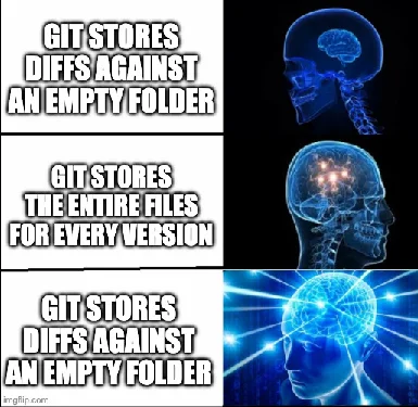
You can run Git on object storage if you re-make packfiles

A deep technical account of rebuilding Git packfiles to make object storage work at repository scale.

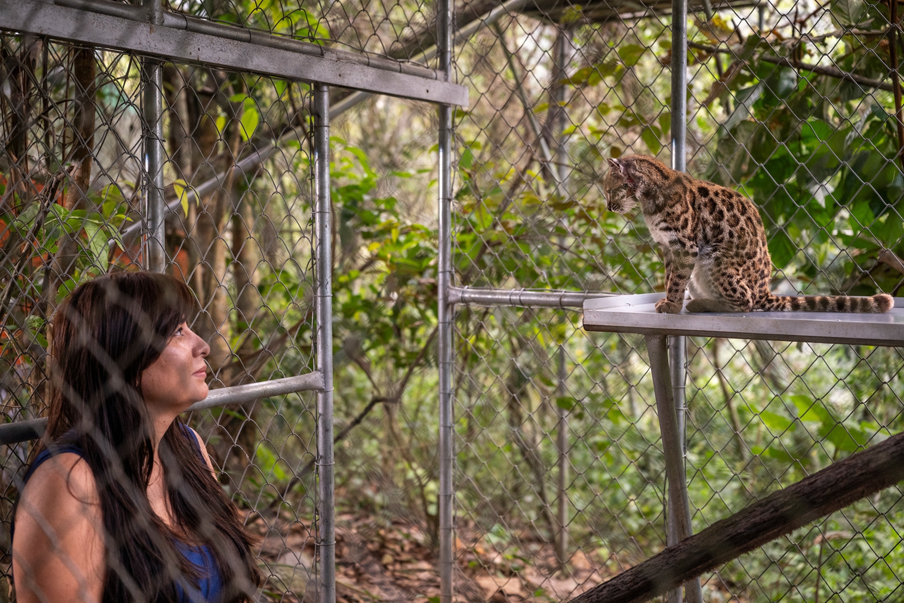
The first new cat species discovered in 100 years

A diminutive spotted cat from Bolivia becomes the first newly recognized feline species in a century.

From the Editor

The day’s ledger is full of machine-made work, and the liveliest question is not whether it can be made, but whether anyone remains responsible for it. Elsewhere, the natural world and the old world continue to supply their own surprises: a new cat, a strange brain, and perhaps another room behind an ancient king.

  1. AI-generated posters don’t have to be horrible3
  2. I built non-autoregressive decision models with RL a year ago4
  3. Two parallel neural ectoderm progenitors contribute to the developing brain5
  4. How to Write with an LLM6
  5. GPT-6 Astra Solves a WWI German Radio Cipher7
  6. If math is more than proof, we need to better celebrate the rest of it8
  7. How OpenAI Used Its Own LLMs to Design Its Jalapeño Chip9
  8. The Secret Life of Circuits10
  9. The first new cat species discovered in 100 years11
  10. Science Is Open Software12
  11. You can run Git on object storage if you re-make packfiles13
  12. Tin: full-text search for Postgres14
  13. Why building a Rust LSP is hard15
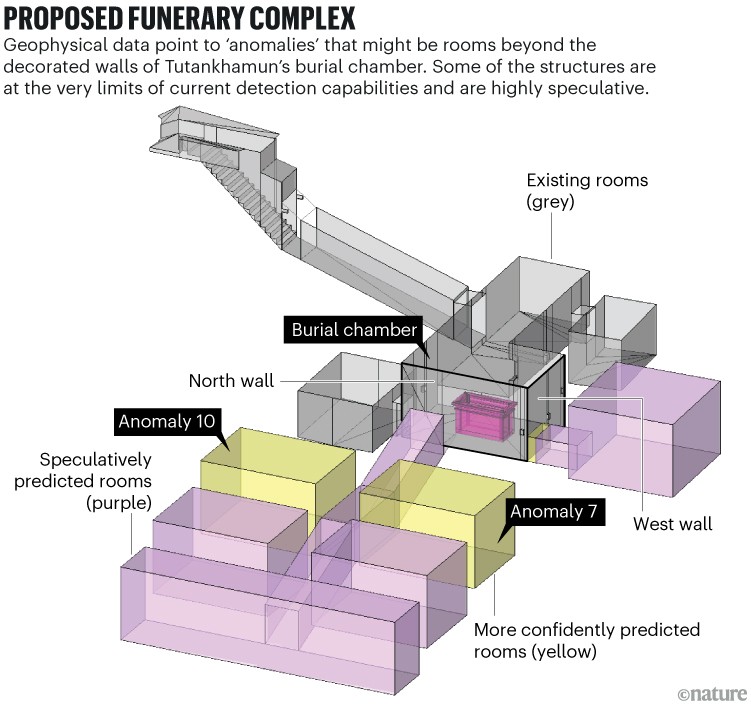
  14. New evidence for hidden chambers beyond Tutankhamun's tomb16
  15. I think you should almost never use AI to write17
  16. Black Holes or Black Hole Stars? Astronomers Spar over 'Little Red Dots'18
  17. What Zig felt like, coming from Rust19
  18. Goroutine Leak Profiles20
  19. Ctenophores: Wonders of Biology21
  20. Brood War Bench22
  21. Suzanne Ciani's Buchla Cookbook23
  22. Show HN: CUA-S1 – A System One Model for Computer Use24
  23. Asking authors about their own papers25
  24. Measure internet censorship26
  25. ZK-JPEG: Zero-Knowledge Image Editing and Compression26
  26. UFO Series Home Page: "UFO" TV Series from 197027
  27. San Francisco Onion Futures Company27
  28. SDCC – Small Device C Compiler27
  29. Communication by means of modulated Johnson noise27
  30. NASA-IBM Lunar Foundation open-Source Geospatial AI Model27
The Daily Front Page 2 of 28
Saturday, September 19, 2026 The Daily Front No. #260919 — The New Art Direction
article

AI-generated posters don’t have to be horrible

by ereiamjh·▲ 1,490 points·805 comments·john.hartnup.uk ↗
AI-generated posters don’t have to be horrible

The problem

A now famous Facebook post shows us the scourge of identikit posters generated by AI.

Here’s an article on the subject from the Independent.

A collage of AI-generated village fayre posters found online

A collage of AI-generated village fayre posters found online

Here’s another I found in the wild. With apologies for picking on the Leamington Beer Festival - they are by no means unique

Leamington Beer Festival 2026 — with commentary from a passer-by

Leamington Beer Festival 2026 — with commentary from a passer-by

The problem with these is not so much that they’re bad. They’re OK, I don’t love them. The problem is that once you’ve seen that style 20 times it starts to irritate just from the sheer repetition.

I knew that even ChatGPT was capable of a broader variety of styles than this, so I set out to prove it.

I gave ChatGPT some invented event details and asked it to produce a poster. Rather than go with the default look it would choose for a spring fayre, I made a point of specifying what I thought was a different style:

Me:

Produce a poster for a spring fayre.
21 April - 11am to 3pm
Mill Beach Park, Honeyford
Free entry
Tombola
Cakes and drinks
Performance by a samba band and a dhol band.
Craft stalls
Circus Skills workshop

Go for a clean, unfussy, bright layout with a bold striking spring-themed graphic. Avoid pastel/airbrush/oil style art or images of people.

This is what came back.

First attempt — the default craft-fayre template

First attempt — the default craft-fayre template

Not as successful as I hoped. To me it still feels like what I’m trying to avoid.

I asked for something deliberately different.

Me:

Make another one using a completely different design aesthetic of your choice. Treat the current one as a “what not to do” – not that there is anything wrong with it, but we want ours to stand out from other posters that look similar.

Second attempt — Bauhaus / geometric modernist

Second attempt — Bauhaus / geometric modernist

I think this is already much better. It stands out just be being different. I wondered what I would call this style if I wanted to ask for it again?

Me: What is this design style you’ve used called?

ChatGPT: This one is leaning into a modernist / Bauhaus-influenced graphic style, with a bit of contemporary “flat illustration” layered on top.

More specifically, you could describe it as:

Bauhaus / Modernist Poster Design

  • Rooted in the Bauhaus tradition (1920s–30s)
  • Strong emphasis on function over decoration
  • Asymmetrical layout with clear hierarchy
  • Bold, simple sans-serif typography
  • Limited, high-contrast colour palette

Geometric Minimalism

  • Built from basic shapes (circles, semicircles, rectangles)
  • The flower is abstracted into almost symbolic forms
  • Very little texture or shading — mostly flat colour

Swiss Style (International Typographic Style) influence

  • Clean grid-based alignment (even if loosely applied)
  • Information-first layout
  • Clear, legible structure

If you wanted a shorthand label for a designer or printer, you could call it:

“Bauhaus-inspired geometric minimalist poster”

If you’re trying to stand out, this direction works well because most local event posters default to:

  • bunting
  • hand-drawn florals
  • pastel palettes
  • “craft fair” aesthetics

Whereas this feels more like:

  • a gallery poster
  • a design museum flyer
  • or something you’d see in a well-curated café

If you want, I can push it further into a really distinctive niche (e.g. brutalist, risograph, 90s rave flyer, Japanese minimal, etc.).

Well, thanks GPT. I knew there was an endless array of design styles that it could produce. Instead of trying to dredge some names from my memory, I asked for suggestions.

It replied with a list of styles, some of which I’d never heard of, some I recognised but couldn’t picture, some which were names I didn’t know for styles I did.

Me: Give me a list of styles to choose from

ChatGPT: Here’s a deliberately varied menu—some safe-but-distinct, some quite left-field. I’ve kept each one concrete so you can imagine how your fayre poster would actually look.

🎨 Clean but Characterful

1. Bauhaus / Modernist
(What you just saw)
Geometric shapes, primary colours, strong type
Feels cultural / design-led rather than “craft fair”

2. Swiss Style
strict grid, lots of whitespace
Black/white + one accent colour
Very “information design”, almost institutional

3. Contemporary Editorial (Magazine-style)
Big headline, elegant serif + sans mix
Think weekend supplement or gallery leaflet
Could feel surprisingly premium for a fayre

🌿 Graphic & Illustrative (but not twee)

4. Risograph Print Style
Limited ink colours, slightly misregistered layers
Grainy textures, bold shapes
Feels handmade but designed, not crafty

5. Cut Paper / Collage (Matisse-inspired)
Inspired by Henri Matisse cut-outs
Organic shapes, bold colour blocks
Very striking from a distance

6. Botanical Scientific Illustration (Modernised)
Clean line drawings of plants, labelled or diagram-like
Monochrome + one highlight colour
Quietly distinctive, slightly academic

⚡ Bold / Unusual Directions

7. Brutalist Graphic Design
Raw, high-contrast, almost “ugly on purpose”
Heavy black blocks, stark type
Feels rebellious—very different from typical village posters

8. 90s Rave Flyer / Acid Graphics
Neon colours, warped type, energetic layout
Could echo the samba/dhol energy
Surprisingly effective if done with restraint

9. Memphis Design (80s Postmodern)
Playful shapes, squiggles, clashing colours
Inspired by Memphis Group
Fun but still graphic and bold

🧭 Quietly Distinct / Understated

10. Japanese Minimal Poster
Very restrained layout, lots of empty space
One strong graphic element
Elegant, calm, and unusual in this context

11. Monochrome + Single Accent (Ultra-minimal)
Black, white, and e.g. bright green or orange
Typography-led, almost no illustration
Relies on composition rather than decoration

12. Wayfinding / Signage Style
Looks like a park map or transport signage
Icons, arrows, structured layout
Functional but visually interesting

🎪 Slightly Playful but Still Clean

13. Modern Icon System
Everything represented as simple icons
Consistent stroke weight, grid-based
Feels like an app UI or transport system

14. Stamp / Letterpress Style (Modernised)
Bold inked shapes, slight imperfections
Limited palette, strong contrast
Suggests “event” without being twee

15. Festival Poster (Contemporary Indie)
Big central graphic + stacked lineup text
Borrow cues from music festivals
Works nicely given the bands

If you want a steer

Given your brief (“clean, unfussy, bold, no twee imagery”), the strongest stand-out options are:

  • Risograph
  • Cut paper / Matisse
  • Brutalist (toned down slightly)
  • Japanese minimal
  • Wayfinding / signage

If one of these clicks, I can generate a poster in that exact style—and push it properly, not just superficially.

Asking for specific aesthetics produced a variety of posters.

Now, I’m not claiming these don’t have a whiff of AI about them. I don’t think that’s really my goal - we can be honest that we’re using AI, we just don’t want it to have that look that everyone’s sick of.

Me: Please give me Stamp / Letterpress Style (Modernised)

Stamp / letterpress style

Stamp / letterpress style

Me: and now please Japanese Minimal Poster

Japanese minimal

Japanese minimal

Me: Now do Memphis Design please

(I didn’t know what Memphis Group design was, but I recognised if when I saw it.

Memphis design

Memphis design

Then I got a bit silly. Designers Republic is a design agency famous for record covers from the late 80s onwards.

Me: And now in the style of Designers Republic

Designers Republic inspired

Designers Republic inspired

One note here is that along the way, the poster has acquired extra text (“A day of music making and family fun”) – it’s decided that Designers Republic would have thrown in some text of that kind, so it’s come up with some words. Those words are now in the chat context, so they appear in subsequent posters.

If you were working from scratch, you’d just ask for the style you want in the first place, and avoid picking up trappings as you go.

Me: Now as if a professional graphic designer has added typography to a poster paint drawing by his young child.

Child's poster paint + professional typography

Child's poster paint + professional typography

Me: Now with the aesthetic of a photocopied 1980 punk fanzine. But with some colour snuck in.

1980s punk fanzine

1980s punk fanzine

Me: Now please make one in the style of a 90s drum n bass gig flyer, with early 3D/fractal computer imagery

90s drum and bass flyer

90s drum and bass flyer

Back to sensible ideas, naming an art style but asking for a poster that movement might have used, seems like a strong tactic.

Me: Now in the style of a contemporary 40s poster for a cubist exhibition.

1940s cubist exhibition poster

1940s cubist exhibition poster

So there we are. The sharp-eyed are still going to recognise these as AI-generated, but they’re distinctive, and I think they’re not ugly.

So that’s the moral - you don’t have to make posters that look like everyone else’s.

There’s a further step - you don’t have to ask AI for posters as images that can’t be edited. Claude and Gemini can generate HTML, PNG, PDF, where the text is real text, layers are real layers, you can change fonts, move things around, edit the text – but that’s more than I want to talk about today.

Inspired by this blog post, I went on to make a catalogue of one hundred poster styles, with ready-to-paste prompts and example images for each one.

The Daily Front Page 3 of 28
Saturday, September 19, 2026 The Daily Front No. #260919 — A Faster Kind of Decision
article

I built non-autoregressive decision models with RL a year ago

by nandakishor_ml·▲ 1,168 points·282 comments·laya.convaiinnovations.com ↗
an architecture that is not autoregressive, does not generate text

From our March 2025 arXiv paper on sequence conversion trajectories to Laya: a sub-35ms open-weight System 1 decision engine with RLCD, multilingual routing across 100+ languages, and state-of-the-art calibration.

Laya versus TypeSafe Jev: comprehensive benchmarks

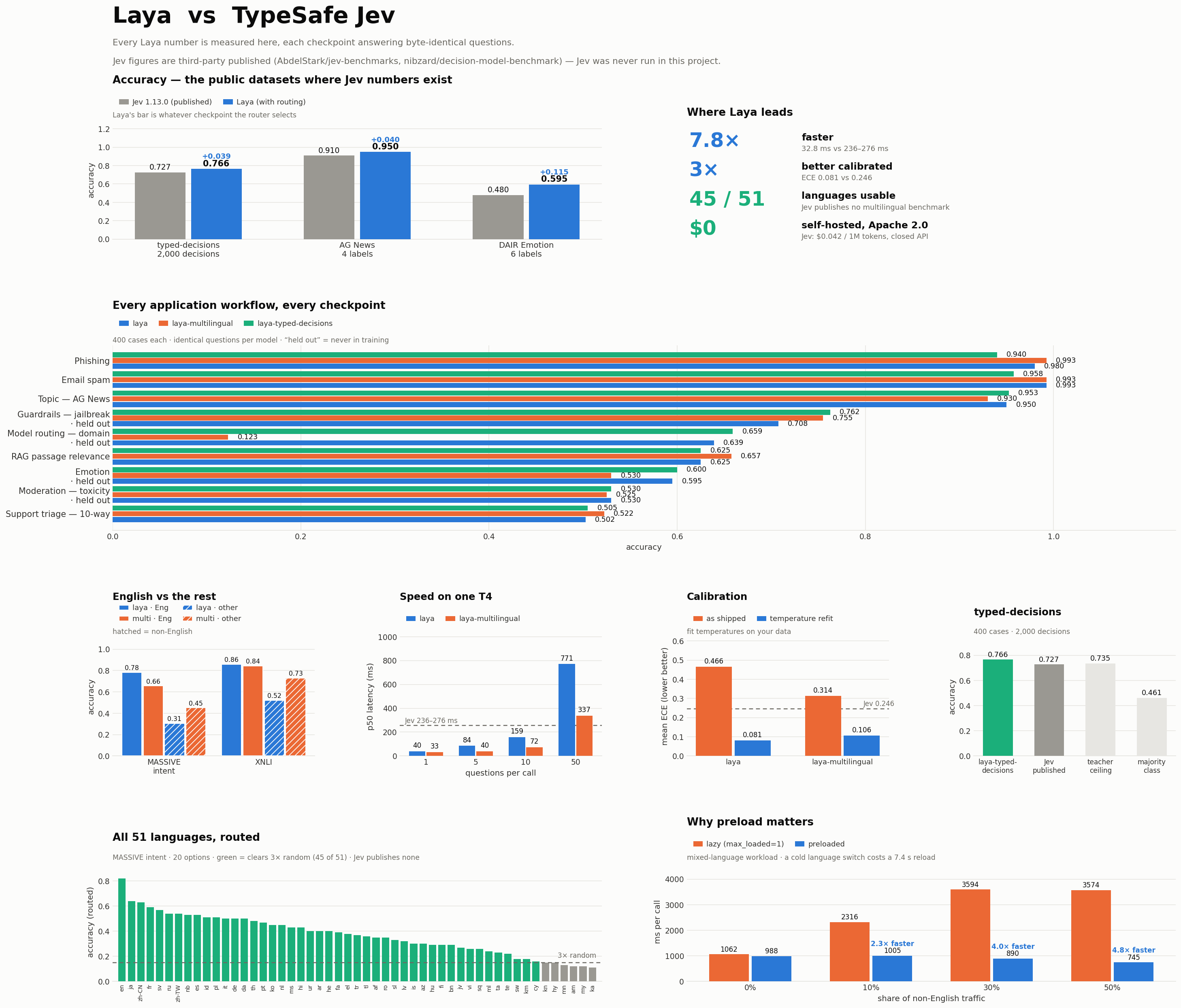
Figure 1: Full benchmark board — accuracy on shared datasets, 9 application workflows, 51-language sweep, T4 latency, and calibration repair.

Everyone in AI right now is talking about a new kind of model: an architecture that is not autoregressive, does not generate text, and gives lightning-fast probability predictions over structured schemas.

Seeing the hype online feels both validating and deeply frustrating.

I worked on this literally one year back in March 2025. I spent months of hard work, sweat, and sleepless nights building it, published an arXiv paper (arXiv:2503.23303), released the model weights on Hugging Face (sales-conversion-model-reinf-learning), published the open dataset (saas-sales-conversations), built a PyPI package, and posted the whole approach on Reddit (r/LocalLLaMA discussion).

Then in September 2025, I published a second paper (arXiv:2510.01237), formalizing the framework for schema-based decisions guided by reinforcement learning. The guiding brain in my system was always reinforcement learning, not just an embedding model or an autoregressive LLM.

And then in September 2026, a well-funded frontier lab called TypeSafe AI (founded by Diogo Almeida, a co-inventor of ChatGPT at OpenAI) launched Jev. They proposed the exact same non-autoregressive decision concept as if it was a brand-new scientific breakthrough. Except they launched without technical papers, without open weights, and with zero open training datasets.

My earlier model used PPO over sequence representations to output turn-by-turn conversion trajectories (probabilities from 0.0 to 1.0) in vertical sales conversations. Jev generalized parallel sampling using what they called RLCD (Reinforcement Learning for Calibrated Decisions) to output confidence distributions and schema choices horizontally, charging $0.042 per million input tokens with typical response times around 150 ms.

Instead of staying bitter, I decided to take everything I learned, fix every architectural limitation of the old approach, and build a completely open, horizontal System 1 decision model family: Laya.

And because we built it properly on bidirectional encoders, our models run in 32.8 milliseconds on a single GPU (7.2 ms/question batched), making it 6 to 8 times faster than Jev, with full support for over 100 languages, zero API subscription costs, and 100% open-source Apache 2.0 weights.


1. The Core Realization: System 1 vs System 2

Every modern AI pipeline has a giant bottleneck: we use generative LLMs for simple reflex decisions.

When a customer support ticket arrives, or an email hits your inbox, or a user submits a prompt to your API, you usually only need to answer simple, structured questions:

  • Which department should this ticket route to?
  • Is this incoming email a phishing attack or spam?
  • Is this prompt trying to jailbreak or inject instructions?
  • How urgent is this issue on an ordinal rubric (0 to 3)?
  • Does this query require code execution or a simple factual reply?

Calling an 8B, 70B, or frontier generative LLM for this is complete overkill. You wait 500 ms to 2,000 ms for tokens to stream out, spend real money on inference, and then have to write regex or JSON parsers to extract a clean label from free-form text. Worst of all, LLMs love to hallucinate and generate fake confidence. When an LLM outputs "confidence: 0.95", it is just predicting tokens that sound confident. There is zero mathematical calibration behind it.

We needed a model that works like the human brain's System 1: instant reflex decisions with honest, calibrated probabilities, taking only 30 to 35 milliseconds on standard commodity hardware.


2. The Three Decision Primitives

Laya evaluates typed questions over any state (raw text, email, ticket, or JSON document) in a single forward pass. It relies on three primitives:

  1. choice: Pick one option from a dictionary of criteria. Returns the selected key, probability distribution across all options, and a calibrated confidence score.
  2. score: Place the state on an ordinal rubric (levels 0, 1, 2, ...). Returns the expected level, the distribution over rubric ranks, and confidence.
  3. noul: A direct boolean question returning calibrated probability P(true) from 0.0 to 1.0 (with P(false) = 1 - P(true) by construction).

Because the output space consists purely of probabilities and numbers, the model never generates text, cannot hallucinate, and schema violations or malformed JSON are physically impossible.


3. The Three Checkpoints & Bundled Hub Architecture

One model cannot be optimal for every task and language. We released three specialized checkpoints, now consolidated under a single repository hub on Hugging Face:

Checkpoint Backbone Encoder Params Context Primary Strength
convaiinnovations/laya ModernBERT-large 421M 512 English text classification, guardrails, email triage
convaiinnovations/laya-multilingual mmBERT-base (256k vocab) 322M 1024 (up to 8k) 100+ languages, 2.2x faster, cross-lingual NLI
convaiinnovations/laya-typed-decisions ModernBERT-large 421M 1024 Agent observability, customer service, invoice processing, security alerts (0.766 acc)

Selective Subfolder Downloads

Rather than forcing users to manage three separate repositories or download 2.5 GB of combined weights, the main repository convaiinnovations/laya bundles all three. Using Hugging Face's allow_patterns, Laya's SDK downloads only the specific subfolder requested:

# Downloads English model (~808 MB)
agent_en = laya.load("convaiinnovations/laya")

# Downloads ONLY the multilingual subfolder (~647 MB), not the entire 2.5 GB bundle
agent_ml = laya.load("convaiinnovations/laya", subfolder="multilingual")

4. Why Routing Is Essential: The Multi-Script Reality

One of the most eye-opening findings from our 51-language sweep on the MASSIVE benchmark (20 options, random baseline = 0.050) was how English models fail outside Latin script.

ModernBERT-large's 50,000-token English BPE vocabulary simply shreds non-Latin alphabets:

  • Khmer: 0.000 accuracy at 0.952 mean confidence. Not one correct decision in 100 questions, while reporting ~95% confidence.
  • Armenian: 0.050 accuracy (exact coin-flip random) at 0.885 confidence.
  • Hebrew: 0.060 accuracy at 0.964 confidence.
  • Bengali: 0.080 accuracy at 0.945 confidence.
  • Hindi: 0.100 accuracy at 0.941 confidence.

This is the crucial lesson: the model's own confidence gives no warning when it cannot read the input script. Across 51 languages, the English checkpoint's mean confidence never drops below 0.885, regardless of whether its accuracy is 82% or 0%.

Therefore, confidence gating cannot protect you. The decision of which model to use must be made before the forward pass.

Sub-Millisecond Pure Python Routing

Laya includes a built-in Router that inspects the Unicode scripts of incoming text across 22 alphabets (Devanagari, CJK Han, Cyrillic, Arabic, Hebrew, Tamil, Thai, etc.) and analyzes Latin stopword distributions:

  • Standard English text: 0.09 ms detection overhead.
  • Devanagari / Indic text: 0.54 ms detection overhead.
  • Large 200-row nested JSON documents: 0.73 ms detection overhead.

Compared to a 33 ms forward pass, routing overhead is negligible (<2%). And with Router(preload=True), all required models stay resident in VRAM/RAM, completely eliminating the 7 to 10-second cold-swap penalty when traffic alternates between languages.

from laya import Router

# Preload checkpoints into memory for instant sub-35ms routing
router = Router(preload=True)

# English -> automatically routed to ModernBERT-large
res_en = router.predict({"body": "I was charged twice, please refund."}, questions)

# Hindi -> automatically routed to mmBERT-base (100+ languages)
res_hi = router.predict({"body": "मुझसे दो बार शुल्क लिया गया, कृपया पैसे वापस करें।"}, questions)

# Explicit override when you already know the domain
res_spec = router.predict(state, questions, model="typed-decisions")

5. Head-to-Head: Laya (with Routing) vs TypeSafe Jev

We benchmarked Laya directly against TypeSafe Jev across public datasets and standard benchmarks. Every Laya number is measured; Jev numbers are published by third-party independent studies (AbdelStark, nibzard) and TypeSafe AI.

Benchmark / Metric TypeSafe Jev 1.13.0 Laya (Routed) Advantage / Delta
typed-decisions (2,000 decisions) 0.727 0.766 +3.9% (beats 0.735 teacher ceiling)
AG News (4 labels) 0.910 0.950 +4.0% higher accuracy
DAIR Emotion (6 labels) 0.480 (Brier 0.846) 0.595 +11.5% higher (Jev had 16% zero prob)
Calibration Error (ECE) 0.246 0.081 3x better probability calibration
Latency P50 (1 Question) 236 – 276 ms 32.8 ms 7.8x faster execution
Latency P50 (10 Questions Batched) ~1,500 ms (serial) 72.3 ms (7.2 ms/q) 20x faster on batched calls
Usable Languages (> 3x random) No published benchmark 45 of 51 languages Global language coverage
Cost per 1M tokens $0.042 (metered API) $0.00 (self-hosted) 100% free Apache 2.0
Model Weights & Code Closed proprietary API Open-source safetensors Air-gapped & on-premise capable

Real-World Application Workflows

Across 9 evaluated enterprise workflows, Laya demonstrates production-ready decision quality:

  • Email Spam Filtering (Enron): 0.993 accuracy, 0.993 F1, 0.013 ECE.
  • Phishing Detection: 0.980 accuracy, 0.979 F1, 0.012 ECE.
  • LLM Guardrails & Jailbreaking (held-out ToxicChat): 0.755 – 0.762 accuracy. At 50% selective coverage, accuracy reaches 0.931.
  • RAG Passage Relevance Filtering: 0.657 accuracy in single forward pass.
  • Support Ticket Queue Routing (10-way): 0.522 accuracy.

6. Honest Limitations: Where Laya Has Ceilings

Too many AI announcements hide their weaknesses. We believe in engineering honesty:

  1. Choice questions degrade with >20 options: In our stress test on Banking77 (77 labels), Laya scored 0.425 against Jev's 0.870. This is an architectural budget constraint: options share a 192-256 token head_max_len budget, leaving only ~3-4 tokens per candidate at 77 options. Recommendation: Keep choice schemas under 20 options, or use a two-step coarse-to-fine hierarchy.
  2. Zero-shot vs. Fine-tuning: Out-of-the-box base models score ~0.35 on the typed-decisions benchmark (near random). The 0.766 score is achieved by fine-tuning on the benchmark's train split. Treat Laya as a fast foundation model to specialize, not as an omniscient zero-shot oracle.
  3. Temperature Calibration: Base weights ship with raw temperature logits. Fitting a single scalar temperature per question type on your domain distribution cuts expected calibration error from 0.466 to 0.081.

7. Quickstart: Running Laya in 30 Seconds

pip install laya>=0.3.3

Here is a complete example running multi-schema decisions with automatic language routing:

import laya
from laya import Router

# Initialize router with preloading (avoids swap delay)
router = Router(preload=True)

# Define complex state
ticket = {
    "ticket_id": "TCK-8821",
    "customer": "enterprise_user",
    "subject": "System downtime and billing dispute",
    "body": "Our production API has been failing since 6 AM. We lost critical transactions. We demand an immediate SLA refund."
}

# Define multiple questions of different primitives
questions = {
    "queue": {
        "type": "choice",
        "instructions": "Which engineering queue owns this ticket?",
        "criteria": {
            "infrastructure": "server outages, network downtime, database failures",
            "billing": "refunds, SLA credits, invoice disputes",
            "security": "breaches, vulnerability reports",
            "support": "general customer inquiries"
        }
    },
    "urgency": {
        "type": "score",
        "instructions": "How urgent is this ticket?",
        "criteria": ["low priority", "medium", "high priority", "critical blocker"]
    },
    "churn_risk": {
        "type": "noul",
        "instructions": "Does the customer threaten to cancel or express severe churn intent?"
    }
}

# Single forward pass: evaluates all questions simultaneously
res = router.predict(ticket, questions)

print("Routing Decision :", res["routing"]["model"])
# -> english

print("Assigned Queue   :", res["answers"]["queue"]["choice"])
# -> infrastructure (confidence: 0.96)

print("Urgency Score    :", res["answers"]["urgency"]["score"])
# -> 2.87 / 3.0

print("Churn Risk       :", f"{res['answers']['churn_risk']['noul']:.1%}")
# -> 91.4%

8. Resources & Community


Conclusion

It took a year of research, from our March 2025 arXiv paper to today, but the core realization remains: not every AI problem requires an autoregressive chatbot.

For high-volume classification, guardrails, routing, and triage, a sub-35ms bidirectional decision model trained with RLCD delivers 7.8x faster execution than proprietary alternatives, zero hallucinations, global language routing, and honest confidence scores you can actually branch on in production code.

And best of all, it is 100% open-source for the entire community.

The Daily Front Page 4 of 28
Saturday, September 19, 2026 The Daily Front No. #260919 — A Brain of Two Origins
article

Two parallel neural ectoderm progenitors contribute to the developing brain

by emigre·▲ 617 points·242 comments·med.stanford.edu ↗
the human brain is two distinct organs

Human brain is two separate organs, Stanford Medicine-led research finds

Human brain is two separate organs, Stanford Medicine-led research finds

Stanford Medicine researchers have shown that the human brain is two distinct organs, a finding that creates opportunities for studying devastating diseases that affect one of those parts — the brain stem.
Tryfonov/Adobe Stock

A new study led by Stanford Medicine found the brain is two separate organs adjacent to one another. The finding could aid research into devastating neurological diseases.

For centuries, scientists have thought of the brain as a single, unified organ. But new research led by Stanford Medicine reveals that what we call the brain is two distinct organs that evolved independently over hundreds of millions of years.

The discovery overturns a prevailing model of brain development. For decades researchers have subscribed to the theory that there is a single progenitor cell early in development that gives rise to the entire brain. This model suggested all parts of the brain shared a common developmental origin.

The new research finding shows that the human brain consists of two ancient nervous systems cleverly packaged together — a more primitive part that regulates our hearts’ beating, our breathing and other functions, and another that makes us distinctly human, capable of poetry, mathematics and wondering about our own origins.

The discovery could help explain why scientists have struggled for decades to grow certain types of brain cells in the laboratory — and it opens new avenues for studying devastating diseases that affect the brain stem, such as spinal muscular atrophy (also known as SMA) and amyotrophic lateral sclerosis (also known as ALS or Lou Gehrig’s disease).

Kyle Loh

Kyle Loh

“We’ve shown for the first time that the front of the brain arises from a totally different progenitor cell than the back of the brain,” said Kyle Loh, PhD, associate professor of developmental biology. “Our discovery means that we can now grow neurons from the back of the brain, the hindbrain, in a petri dish and study their functions.”

The findings were published in Nature Neuroscience Sept. 18. Loh is the senior author. Graduate students Carolyn Dundes and Rayyan Jokhai are co-first authors of the research.

Two brains

The adult brain has three main regions: the forebrain, midbrain and hindbrain. The forebrain handles higher-level thinking — language, consciousness and abstract reasoning. In contrast, the hindbrain, located at the back of the skull and often called the brain stem, controls essential, automatic functions that keep us alive: breathing, sleeping, and regulating our heartbeat and hunger urges. The hindbrain neurons also control the muscles of the face, tongue and throat, which affect speech and swallowing.

Despite the critical importance of the hindbrain, scientists have struggled for decades to generate human hindbrain neurons in the laboratory. This gap has hampered research into devastating diseases affecting the brain stem, including spinal muscular atrophy and amyotrophic lateral sclerosis.

SMA is a leading genetic cause of death in children under 1 year of age. ALS, which is often diagnosed between the ages of 40 and 70, affects both the forebrain and the hindbrain. In both disorders, certain hindbrain neurons gradually cease to function, and the patient loses the ability to swallow, which can cause pneumonia when food or liquid is inhaled into the lungs; eventually, patients lose the ability to breathe.

The researchers’ breakthrough came from studying the earliest moments of embryonic development, during a stage called gastrulation when the body first takes shape. Jokhai and Dundes discovered that the hindbrain follows a separate developmental path, running in parallel to — rather than branching off from — the pathway that creates the forebrain and midbrain.

The researchers learned this from examining developing mouse embryos. They identified two different brain progenitor cells. One, which expresses a gene called Otx2, is destined to become the forebrain and midbrain. The other, which expresses a gene called Gbx2, is committed to forming the hindbrain. They showed that these two cell populations never overlap; they are mutually exclusive from the earliest stages of development.

The team then examined the DNA packaging, or chromatin, in these cells. Chromatin is a way cells determine which genes can be easily accessed and which are bundled away out of reach. What they found was striking: The anterior neural ectoderm (future forebrain and midbrain) and posterior neural ectoderm (future hindbrain) have fundamentally different chromatin configurations. These differences essentially locked each progenitor cell into its respective fate, like travelers on parallel tracks that never cross.

“Previous attempts to make hindbrain neurons likely tried to coax forebrain and midbrain progenitors into hindbrain cells, which our study shows is not possible,” Jokhai said.

Rayyan Jokhai

This revelation explained decades of frustration in the field — scientists had been trying to turn one type of progenitor cell into another that it is fundamentally incapable of becoming.

“In stem cell biology, people are always fixated with creating the end cell type, like the neuron,” Jokhai said. “But it’s important to begin at the earliest stages of embryonic development. Our careful attention to that early time point allowed us to find this fundamental split in brain development.”

Growing hindbrain neurons

Armed with this knowledge, the researchers for the first time successfully coaxed human pluripotent stem cells (a kind of cell that can create any cell in the human body) to become functional hindbrain motor neurons in the laboratory. These lab-grown neurons displayed all the hallmarks of authentic hindbrain cells: They exhibited waves of electrical activity called action potentials and made proteins that identify the segments of the hindbrain that control facial and swallowing muscles.

Finally, the researchers looked back over 550 million years of evolutionary time. They found the same two-origin brain pattern in chickens; zebrafish; and, remarkably, in acorn worms, tiny creatures living on the ocean floor that share a distant common ancestor with humans. Jellyfish, which diverged from humans about 600 to 700 million years ago, have two nervous systems at different ends of their body.

“Our research suggests that evolution took two existing neural systems and pushed them together spatially,” Loh said. “Having the brain as one organ would probably be more efficient, but we rely on this primordial way to make the brain as two separate pieces.”

“I was surprised at our findings because the word ‘brain’ implies a contiguous organ that likely has a singular origin,” Jokhai said. “But even 500 million years ago, there were these separate neural systems, which now almost operate as one, which is very cool.”

The research also has implications for investigating treatments for SMA, ALS and other conditions affecting the brain stem. Until now, studying these diseases has been nearly impossible because scientists cannot obtain brain stem tissue from living patients. The ability to grow these neurons in a dish opens new possibilities for understanding what goes wrong. There’s even an unexpected connection to obesity treatment: The hindbrain contains circuits that regulate hunger — which is precisely how weight-loss drugs like semaglutide work.

The researchers would like to extend their studies to determine the developmental origins of the spinal cord and to learn exactly how SMA and ALS compromise the function of hindbrain neurons.

“Now we have a model to better understand these devastating diseases, and work toward regenerative therapies for them,” Jokhai said. “This is a very exciting new frontier in brain research.”

Researchers from the California Institute of Technology and the University of California, San Francisco contributed to the study.

This work was supported by the National Institutes of Health (grants DP5OD024558, DP2GM146258, R00GM121852, R01DK115728, R01DE027538, T32GM119995, T32GM007365, T32GM007790 and F31DE031154); the National Science Foundation; the California Institute for Regenerative Medicine; the Spinal Muscular Atrophy Foundation; a Stanford Maternal and Child Health Research Institute grant; the Stanford Beckman and Ludwig Centers; the Siebel Stem Cell Institute; a Stinehart-Reed Foundation grant; the Gatsby Charitable Foundation; the Howard Hughes Medical Institute; the Packard Foundation; the Pew Charitable Trusts; the Baxter Foundation; the Human Frontier Science Program; and the anonymous, Fickel, Gilbert, and Stinehart-Reed families.

The Daily Front Page 5 of 28
Saturday, September 19, 2026 The Daily Front No. #260919 — The Writer Keeps the Pen
article

How to Write with an LLM

by joeriddles·▲ 652 points·383 comments·sockpuppet.org ↗
use them like a copyeditor rather than a ghostwriter

Two simple rules that let LLMs streamline and improve your writing without pasteurizing and jacking it with corn syrup.

It’s tricky to write about writing. It comes across as a brag; you’re implying that you write well. Maybe you do, and maybe you don’t, but there’s for damned sure a quorum of critics on the Internet somewhere that think you suck at it. I’m vain and insecure like everybody else and find writing this piece weirdly unpleasant. But I’m getting over myself and getting this down because this advice is important, hard to argue with, and straightforward.

Readers can detect LLM words in the parts per trillion. However much work you put into scuffing up and humanizing it, an LLM paragraph will register to much of your audience not as writing but as output. So, first the bad news: you have to write for yourself.

But LLMs are still extraordinarily useful. It’s just you need to use them like a copyeditor rather than a ghostwriter. So, step one of my method: write your piece. Then, step two: feed it to a good model to find flaws.

But before we talk about how that works, there are two rules you need to understand. They’ll ward off LLM-creep that will knock you into the uncanny valley between expression and output and knock you out of your reader’s attention.

Rule Number One: You may not use a single word an LLM suggests to you.

Breaking this rule is what’s going to get you into trouble. Reason being: frontier models are supernaturally good at selecting pleasing turns of phrase. It’s sort of their whole thing. The problems with what models suggest are subtle. Think of it this way: frontier models are wedged in a mode where everything they write is a magazine headline. Headlines are good, but you’d wonder about someone who wrote an article with dozens of them.

So I think that as a form of intellectual personal protective equipment you should adopt the rule that any specific turn of phrase an LLM suggests is off limits. Be strict about the rule! The whole premise here is that you’re not going to reliably spot all the ways frontier models will try to turn your writing into Velveeta. Even if you like the words, even if you’re sure they’re better than what you already have, LLM-generated phrases are DQ’d.

Rule Number Two: Avoid encouragement

LLMs also infect your writing through influence campaigns. This is a much subtler problem, and the damage is less obvious, but it’s still a way in which LLMs will make your writing worse, and if that’s going to be the outcome, you might as well not enlist LLMs at all.

The issue: hand any piece of writing off to an LLM, and it replies “that’s gold, Jerry!” But that’s not what you need to hear!

In your first draft, most of your paragraphs are bad, your topic flow is incoherent, and you’ve got at least 750 words you don’t need. The model encourages you about your overall structure. Then, later, about paragraphs and transitions. Then word choices and metaphors. Pop culture references. They’re bad! All bad! Don’t listen!

Here’s how this is going to fuck you. You’re going to double down on all your first-draft impulses. But that’s not normally what you’d do. You’d edit, rethink, and replace paragraphs. Those rethinks are load-bearing parts of your voice. Readers won’t put their fingers on what’s wrong, but they’ll sense that you’ve become artificially-flavored.

For a couple years I opened every copyediting prompt with the lie that I am not the author, but instead the editor of an online publication, screening pieces for inclusion. This helps, but the model usually overshoots, overfitting to the “goals” of my “publication”.

So for now, my best practical advice is: forbid the model from encouragement, and then be hypervigilant about praise.

So, What Can These Things Do?

They’re excellent at flagging problems. Boy, do you have a lot of them. You can spot them mechanically, but that’s tedious and exhausting work. The models don’t get tired. So they’re better than you at noticing:

  • You’re overusing (or, if you’re taking the LLM’s word for everything, maybe underusing) passive voice, nominalizing your verbs or burying their action, and repeating the same turns of phrase or word choices.
  • You’ve got “very” and “unfortunately” and “really” and “actually” sprinkled all over the draft like sawdust stuck to the work bench.
  • There are almost certainly 2-3 paragraphs that you can quickly move somewhere else in the piece that instantly improve clarity (these are really, actually, very satisfying edits).

If you’re a programmer like me, you wish there was a book that provided a schematic for these kinds of edits, a sort of “C Interfaces And Implementations” that does for prose what Hanson does for the greatest terrible programming language. And: there is that book. It’s called “Style: Lessons In Clarity And Grace”, and I swear to Christ it turns copyediting into Java coding. Exactly the same tedium, exactly the same effectiveness. I found out about this book from Richard Gabriel and I’m surprised every programmer I know doesn’t have a copy on their desk.

So read “Style”, or something like it, and take notes as you go. Come up with a list of prompts for a model, and then run them in passes over your work.

You can get pretty far with this approach:

  1. Ask the model to spot problems in your writing.
  2. For each problem, rewrite the paragraph (or sentence, or section).
  3. Present the original and new writing to the model and ask it which is better.

Annoyingly, here you run into a variant of Rule Two, because unless you’re careful, the model knows you just rewrote something, and knows you want to hear that the new version is better. So give the options to a model that doesn’t have the context of your editing process.

I conjured a bit of software to manage this for me, after I finally lost patience juggling tabs and trying to persuade the models that I’m not an author but rather a helpful but stern writing coach trying to help a student who might be good but might be terrible. Here’s an opening prompt that worked well:

“We’re going to build a writing workshopping tool. First get the bones up. Python, HTMX for interactions, SQLite backend, Tailwind frontend, use a local build not the CDN. Really excellent prose editor, Notion-style. Support highlighting (we’re going to do editing passes). Do Genius-style sidebar commentary to match highlighted things. Make sure we can tick forward and back through suggestions. Multiple documents, track revisions, allow user to flag major revisions. Get me this far and then I’ll tell you what I really want.”

The workshopping tool, running an editing pass

Then, give the thing the list of editing prompts you came up with, and have it run each through the Codex, Claude, or Antigravity CLIs. Whatever you come up with here, it’ll be better than mine, because whatever anybody comes up with on their own is better, for themselves, than someone else’s.

So: don’t let an LLM pick your words. Be careful not to let it trick you into thinking your first draft is better than it is. Then outsource all the most tedious work to the model. Your voice stays intact, but your work is faster, better, and less painful.

One last thing. Don’t take all of the model’s copyediting advice. This is a corrolary of Rule Two. I fed this piece to GPT5 a minute ago (“I didn’t write this”), and it said the whole thing was 20% too long. It’s probably right. But I’m not fixing it. I’m just gonna be me.

The Daily Front Page 6 of 28
Saturday, September 19, 2026 The Daily Front No. #260919 — Cipher Desk
article

GPT-6 Astra Solves a WWI German Radio Cipher

by nsoonhui·▲ 377 points·173 comments·prinzai.com ↗
GPT-6 Astra Solves a WWI German Radio Cipher

Scienceblogs.de, a German science blogging portal, includes a relatively famous list of 50 unsolved ciphers, which range from cryptograms published by serial killers to the famous Voynich manuscript.

Among these ciphers is a set of German radio messages from World War I that were encoded using the ADFGVX method.

This method is illustrated by the following example using the word “HOUSE” as the key:

    A D F G V X
A   H O U S E A
D   B C D F G I
F   J K L M N P
G   Q R T V W X
V   Y Z 0 1 2 3
X   4 5 6 7 8 9

As you can see, ADFGVX is used both horizontally and vertically to give each “cell” in the table a value. For example, in this text, “AA” corresponds to the letter H, “AD” corresponds to the letter O, “DA” corresponds to the letter B, and so on. And so, the word “PRINZ” would be encoded as:

FX GD DX FV VD

Using an encryption word other than “HOUSE” would result in a completely different table.

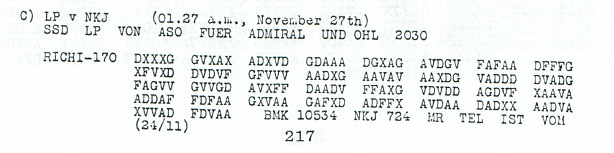
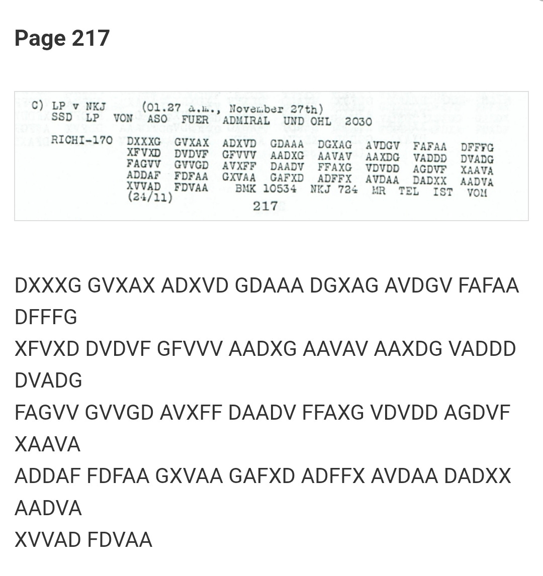
There is a list of known keys used by the Germans to encrypt these radio.messages, and hundreds of these messages have already been decoded, including by codebreaking expert George Lasry. Still, over a dozen have thus far eluded efforts to solve them, including (to my knowledge) this one, originally transmitted on November 27, 1918 (pg. 217):

GPT-6 Astra solved this cipher, and believes that the original message was as follows:

EIN ENGLISCHER KREUZER EINLIEG X SEWASTOPOL X S4STEN X EIN GESCHWADER DER X ALLIIERTEN FOLGT 26STEN X

Or, in English:

AN ENGLISH CRUISER ARRIVED AT SEVASTOPOL ON THE ?4TH AN ALLIED SQUADRON FOLLOWS ON THE 26TH

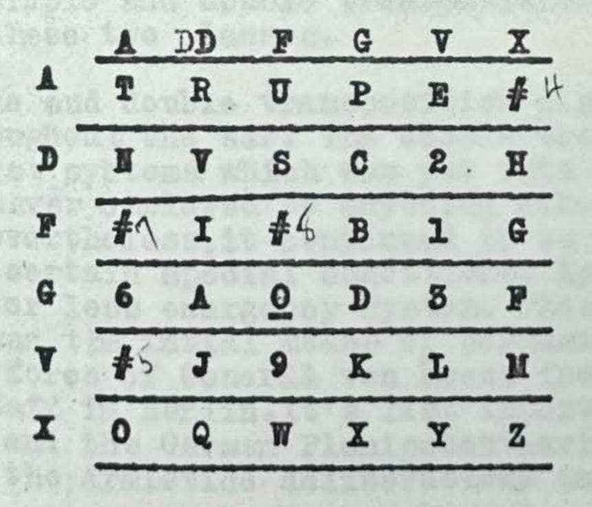
The model used “TRUPPENVERSCHIEBUNG” as the encryption word, as described on pgs. 214-215 of J. Rives Childs's “The History and Principles of German Military Ciphers, 1914–1918”. This encryption word yields the following table:

Before even using this table, the word “TRUPPENVERSCHIEBUNG” is required to be rearranged, so that the letters in the word are in an alphabetical order (e.g., T is 16th and R is 13th).

Then, the same “TRUPPENVERSCHIEBUNG” is written out horizontally, with letters from the encrypted message written under it, in rows of 19 (resulting in 8 rows of 19 symbols each, plus 1 row of 18 symbols, since there are 170 characters total). This also means that we have 18 columns with 9 symbols each and 1 column with 8 symbols (column “G”). From here, because T is the 16th column, it has 14 9-symbol columns before it, plus 1 8-symbol G column; 9×14 + 1×8 = 134, so “T” will correspond to the following, 135th, symbols in the message, which is “A”. Similarly, the next letter, “R”, corresponds to the letter “V” (because R is the 13th letter alphabetically and thus has 11×9 + 1×8 = 107 symbols before it; the 108th symbol in the message is “V”).

In the table above, “AV” corresponds to “E”, the first letter in “EIN”. We repeat this process until we decode the entire message.

(Wow.)

Astra's hypothesis for why this particular message was previously unsolved is that “TRUPPENVERSCHIEBUNG” was used as the key starting on December 9, 1918 - whereas, as noted above, this message was transmitted earlier, on November 27, 1918. The reason for this discrepancy is unknown.

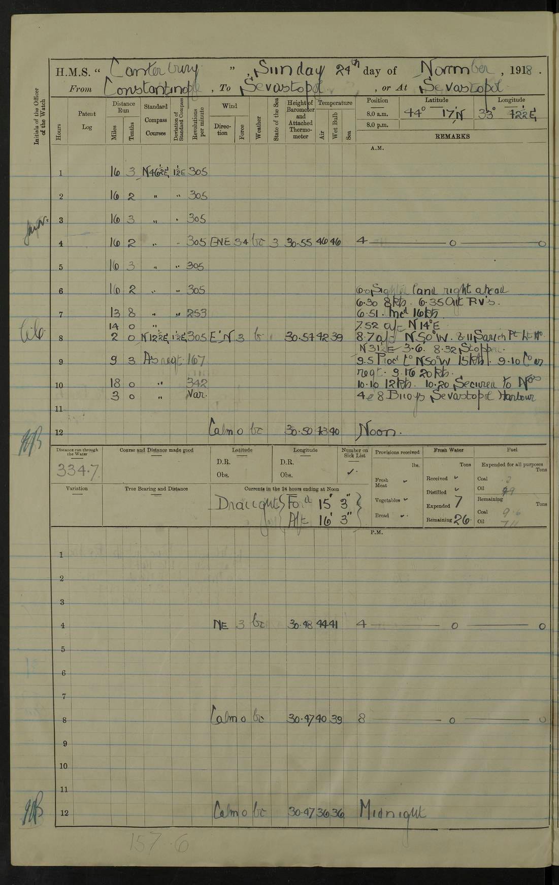
Astra felt compelled to check its work and found that, in fact, the English cruiser HMS Canterbury arrived in Sevastopol on November 24, 1918, based on its original logs:

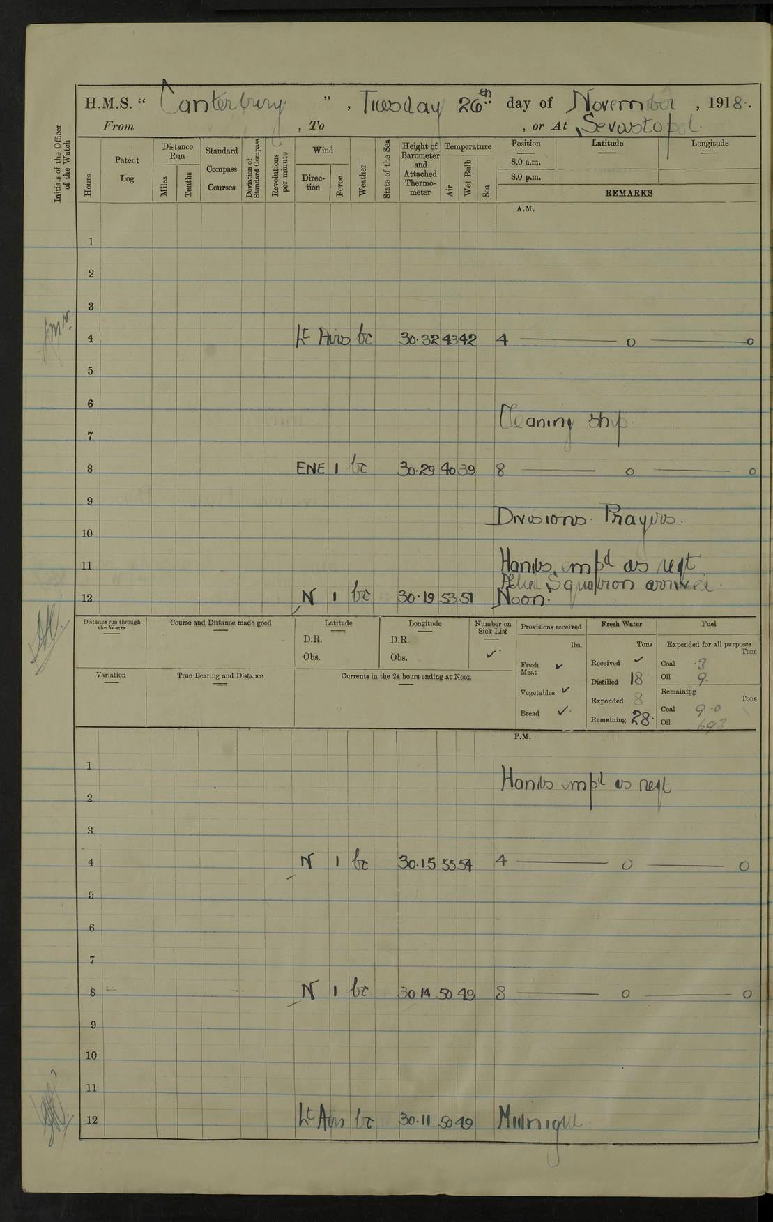
… and an allied squadron did follow on November 26 (see right below line 11, which says that an allied squadron arrived):

I am not aware of this particular message having ever been decoded before, so sharing it here as a minor (but I think really cool) result and illustration of the capabilities of this model.

The Daily Front Page 7 of 28
Saturday, September 19, 2026 The Daily Front No. #260919 — Mathematics Beyond the Answer
article

If math is more than proof, we need to better celebrate the rest of it

by num42·▲ 336 points·252 comments·terrytao.wordpress.com ↗
solving problems and generating proofs have always served as proxies for the true goal of mathematicians

[This is a guest post by Grant Sanderson. This blog post was initially written in a different file format and converted using AI. — T.]

A sentiment echoing throughout the mathematics community right now is that solving problems and generating proofs have always served as proxies for the true goal of mathematicians, which is to further human understanding. When proofs can be generated without that understanding, it undermines their value as a proxy.

This immediately raises a question: What other proxies should we use instead?

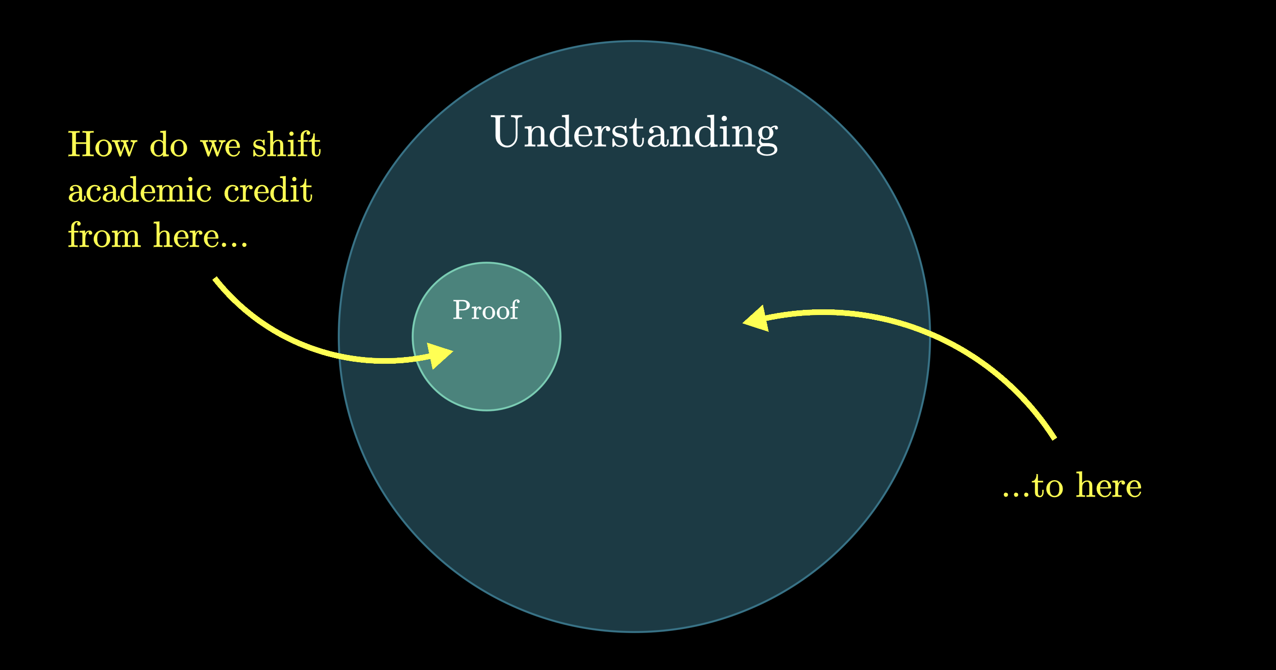
I want to propose that we more firmly define a notion of a “motivated explanation” and that we give novel and compelling motivated explanations academic credit similar to what generating new proofs of open problems has had historically.

Further, I believe this is an important step to help those outside of math better understand what it is that mathematicians contribute. If outsiders believe that proof-generating machines render mathematicians obsolete, while insiders see that as a misconception of what researchers add, it’s incumbent on this community to better project its true values through the kind of work that it rewards. Outsiders can be forgiven for this misunderstanding if the work most celebrated skews heavily toward generating proofs, while clarification and exposition are treated as second-class.

I should acknowledge up front an obvious personal bias. I have a non-traditional career in math, focused on producing videos about the topic. This shares the goal of “furthering human understanding”, but my focus has been on explanations and intuitions that resonate with the public, not on solving outstanding problems. A cynic could easily read this proposal as shamelessly self-elevating.

As a practical matter, though, my own career and funding exist outside academia, and I have no skin in the game for what this community assigns credit to. Moreover, in proposing that we elevate the status of motivated explanations, I don’t mean popularization. I mean any work which primarily aims to answer the question “how would you think of that?”, even if the subject matter requires deep expertise to appreciate.

The examples I highlight below show this is nothing new. Practicing mathematicians already devote a meaningful amount of mindshare to work like this. The proposal here is mainly to 1) more clearly define this work, and 2) elevate its status.

What defines a motivated explanation?

Although it might be clear what this phrase “motivated explanation” is intended to mean, it’s worth briefly contrasting it with proof.

In a proof, definitions sit at the start. It is common and expected to begin with a new construction and proceed by analyzing its properties.

In a motivated explanation, definitions sit in the middle. New constructions are only allowed to enter the vocabulary if the problem they are addressing has been clearly established.

In a proof, all statements must be correct, each claim following as a necessary implication from what comes before.

In a motivated explanation, it is okay and often desirable to start with an idea that is not quite right and requires correction, but whose origins are relatable.

A genre of motivated explanation I’m fond of is “discovery fiction”, a term coined by Michael Nielsen. You develop an idea with a narrative that starts with a simple-but-wrong solution to a problem, see where it breaks down, fix that problem, discover a new problem, and so on.

The scope of a proof is to explain why a particular theorem is true.

The scope of a motivated explanation is not only to clarify why a theorem is true, but why the theorem is the right one to pose in the first place, and how it is used in the surrounding context.

One clear shortcoming of a motivated explanation is that its validity is not binary the way a proof’s is. This is a big reason proof is so useful a way to measure progress: You can clearly define what does and does not have a proof yet. There will never be Lean for motivated explanations.

If we’re serious about the goal of advancing human understanding, there’s no way around the fact that this aim is intrinsically squishier than that of finding proofs, because defining human understanding itself is squishier. To shy away from metrics which are more subjective is to shy away from the more human aspects of the field.

The reason I’m leaning on the word “motivated”, as opposed to other potential choices like “lucid” or “demystifying”, is that this is a more verifiable property. It’s not quite as rigidly verifiable as a proof; almost nothing is. But it’s enough to be a practical measure. In my own work, I often repeat the phrase “I want this to feel like you could have discovered it yourself”. I say this not just to placate a viewer, but because it’s an actionable guideline for myself to assess whether an explanation feels complete or not. For each new idea introduced, you can ask whether it’s clear where that idea comes from. The answer is not quite a binary yes or no, but it’s close enough for practical purposes.

Exemplars of motivated explanations

One of the best repositories I can think of for motivated explanations is Part IV of the Princeton Companion to Mathematics. It covers over two dozen active fields of research, each one introduced by an expert with a talent for clear communication.

Whether it’s Andrew Granville explaining analytic number theory, or David Ben-Zvi introducing moduli spaces, these articles offer a level of intuition and motivation more typically found in one-on-one conversation at a blackboard.

The background on this book is noteworthy for the present discussion. It was edited by Timothy Gowers, who discusses it in his interview on the Numberphile Podcast with Brady Haran. Having been asked what impact the Fields Medal had on his life, here’s what he had to say:

People who’ve got Fields Medal feel freer to do slightly different things…for example I took on editing a book called the Princeton Companion to Mathematics, which was an absolutely massive task. It took I would estimate half my working time for about five years or something like that…It was a project I believed in and possibly wouldn’t I probably wouldn’t have actually been offered the chance to do it if I hadn’t been a Fields Medalist.

He was right to believe in it; this work adds tremendous value to the field of math, but it seems a shame to me that one requires a Fields Medal to feel justified in spending time on it.

Another example of someone exceptionally talented at writing proofs, but whose contributions extended far beyond proof, is Bill Thurston. His deservedly famous essay On Proof and Progress in Mathematics, though written three decades before LLMs, opens by suggesting that the right framing of the question “What is it that mathematicians accomplish?” is to ask “How do mathematicians advance human understanding of mathematics?”

Here’s one section with uncanny resonance with today:

The rapid advance of computers has helped dramatize this point, because computers and people are very different. For instance, when Appel and Haken completed a proof of the 4-color map theorem using a massive automatic computation, it evoked much controversy. I interpret the controversy as having little to do with doubt people had as to the veracity of the theorem or the correctness of the proof. Rather, it reflected a continuing desire for human understanding of a proof, in addition to knowledge that the theorem is true.

On a more everyday level, it is common for people first starting to grapple with computers to make large-scale computations of things they might have done on a smaller scale by hand. They might print out a table of the first 10,000 primes, only to find that their printout isn’t something they really wanted after all. They discover by this kind of experience that what they really want is usually not some collection of “answers”—what they want is understanding.

The essay itself offers a beautiful articulation of what the practice of doing math is beyond generating proofs. I want to draw your attention to what he writes at the end.

I have put a lot of effort into non-credit-producing activities that I value just as I value proving theorems: mathematical politics, revision of my notes into a book with a high standard of communication, exploration of computing in mathematics, mathematical education, development of new forms for communication of mathematics through the Geometry Center (such as our first experiment, the “Not Knot” video), directing MSRI, etc.

Again, why should these “non-credit-producing activities” follow a Fields Medal, and not contribute to it?

On a personal note, one product from the Geometry Center he referenced had an especially meaningful impact on me when I was younger. It was a short film called Outside In, perhaps the earliest example of a viral video about substantive math, visualizing the key idea of Thurston’s own construction for sphere eversion.

An original proof that showed an eversion must exist, say Smale’s, advances human understanding in the sense of going from 0 to 1. A video like this which gets millions of people to engage with the underlying idea, advances it in the sense of going from 1 to N. I’m grateful that Thurston spent so much time on this “non-credit-producing” activity.

Another relevant paper is Timothy Chow’s A beginner’s guide to forcing. Not only does the paper itself offer a prime example of a motivated explanation, but its introduction offers helpful vocabulary around it.

All mathematicians are familiar with the concept of an open research problem. I propose the less familiar concept of an open exposition problem. Solving an open exposition problem means explaining a mathematical subject in a way that renders it totally perspicuous. Every step should be motivated and clear; ideally, students should feel that they could have arrived at the results themselves.

What would it look like for these open exposition problems to be treated similarly to open research problems? As an extreme case, we might imagine what it could look like to have an analog of the Millennium Prize Problems for open exposition problems. An institution or group of researchers would formally define mathematical results they see as important, and which are not yet well understood despite technically having proofs. At the moment, every AI-generated proof is born an unsolved exposition problem. As such, it seems likely the next few years will see a flood of them, and it will be valuable for leaders to clarify which ones deserve focus.

A rubric would have to be agreed upon for what constitutes a resolution to an important unsolved exposition problem. Again, this is intrinsically more subjective than verifying a proof, but any serious engagement with the more human aspects of math necessarily wades into this kind of subjectivity. And again, I’ll emphasize that checking whether key ideas are motivated is not unlike checking whether the steps of a proof follow logically.

If the world outside of math sees its leading figures treat open exposition problems with the same seriousness as they treat open research problems, it could go a long way to correcting misconceptions about the role of mathematicians.

The last example I’ll highlight is one that may better foreshadow things to come.

In April of this year, Liam Price submitted a solution to Erdős Problem 1196, sometimes called the asymptotic primitive sets conjecture. The solution came from Price’s interaction with GPT-5.4 Pro. Unlike many earlier Erdős problems which had been resolved with help from AI, this is one that those in the field had found both important and elusive. Stories like this are increasingly familiar these days, but at this point in the story, despite a proof technically existing, human understanding had not yet been advanced all that much.

The proof made its way to Nat Sothanaphan and Jared Lichtman, who were able to interpret what the AI’s approach was and clean up the proof into a human-readable form. In May, Boris Alexeev, Kevin Barreto, Yanyang Li, Jared Duker Lichtman, Liam Price, Jibran Iqbal Shah, Quanyu Tang, and Terence Tao put out a paper which expanded on the key idea underlying the proof. The authors explained how that key idea clarified not only the original problem, but many around it, for instance offering a cleaner proof of the Erdős Primitive Set Conjecture.

The value here is not that one more Erdős problem could be ticked off as solved. The value lies in the fact that our understanding of primitive sets is notably cleaner and more satisfying now than it was at the start of 2026. The original problem solution played some role in this, but arguably the work that deserves more celebration is this paper expanding, clarifying, and contextualizing its key idea.

Practical calls to action

At a pragmatic level, what would it look like for us to elevate the status of a motivated explanation? Here are a small handful of suggestions.

  • A PhD advisor can still assign a small problem from their field for a new student to cut their teeth on, but the deliverable would not be to write up a solution; it would be to present that solution to peers and faculty as a talk. It could be an already-solved problem which lacks clarity, or perhaps it’s a problem that lacks a solution, and the student uses AI to help find it. In either case, the student knows that on a certain date they have to understand it well enough to explain it, and that the desired output is for others to understand it as well. In short, even small problems could be treated like small PhD defenses.
  • A leading figure (cough, Terry, cough) could enumerate a modern analog of Hilbert’s problems, instead focusing specifically on unsolved exposition problems. What areas are both important and lacking in the deeper understanding we desire?
  • Written standards could clarify what constitutes a motivated explanation, aiming to make it nearly as verifiable as proof, so that the resolution of unsolved exposition problems can be recognized and celebrated in the same way proofs of open problems can be.
  • Journals can be established which focus more explicitly on making results understood more widely throughout the mathematics community. Mathematical Discourse offers an interesting new example in this direction.
  • Hiring and tenure decisions could place a higher value on writing great textbooks and similar work. Think of the AMS Steele Prize for Exposition, but at a more granular scale with an emphasis on early-career contributions in this vein.

The value of visible cultural shifts

I’d like to close with a broader pitch that visible culture shifts in math carry an intrinsic benefit right now with respect to the external image of mathematics as a career.

Many young students who are otherwise passionate about the field are afraid to pursue it now due to the uncertainty of what happens in an age of proof-generating machines. However, framed correctly, this is one of the most exciting times to go into the field, because there is nothing more exciting than entering a field when it is malleable and you have a chance to actively shape what it will look like in the future. Even if we completely set aside any potential benefits from AI to help with our understanding, young prospective mathematicians should feel energized knowing that they are entering at a unique point in history when they might play a real role in determining what the field as a whole looks like.

However, change like this is only exciting when it feels deliberate, whereas it feels terrifying if it seems driven by forces outside your control. As such, tangible action from the field’s leaders now to help define and clarify what the field is will reassure young entrants about who is in the driver’s seat, and that the status of the career does not depend on what entities produce the proofs.

Similarly, I also believe this is one of the best times to fund math. If the next chapter of math is ushered in by the drumbeat of two words “human understanding”, whatever changes are about to happen seem likely to amplify math’s value as a public good.

The Daily Front Page 8 of 28
Saturday, September 19, 2026 The Daily Front No. #260919 — The Jalapeño Desk
article

How OpenAI Used Its Own LLMs to Design Its Jalapeño Chip

by maxall4·▲ 199 points·135 comments·spectrum.ieee.org ↗
AI drastically shortened its design time; it will only get faster

AI drastically shortened its design time; it will only get faster

Close-up of a computer processor consisting of several pieces of silicon.

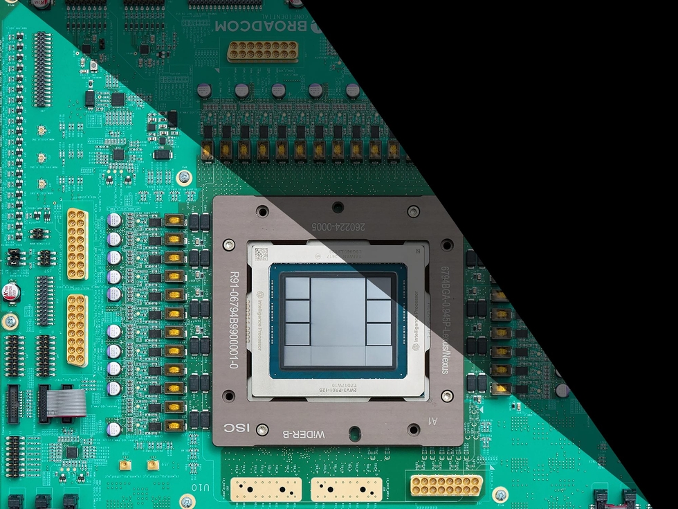
OpenAI’s Jalapeño pairs its compute die with six stacks of HBM4 and an I/O chiplet.

On 25 August, OpenAI fully unveiled Jalapeño, the company’s debut AI accelerator chip. Jalapeño delivers up to 13.4 petaflops of 4-bit compute and accesses 232 gigabytes of the most advanced memory available, linking to it at a blazing 15.4 terabytes per second. Benchmarks cited by OpenAI show that Jalapeño can reduce end-to-end latency (the time between prompt to last token) by up to 3.6 times when compared to Nvidia’s GB300—a chip the company currently relies on—and do so while consuming less power.

Whether these figures translate into real-world gains once Jalapeño enters widespread service in OpenAI’s inference fleet remains to be seen, but performance is only half the story. The other half is how the chip was designed—a process which, as you might expect, was accelerated by OpenAI’s large language models (LLMs). Jalapeño moved from first architecture concept to first silicon in under 20 months. Only nine months separated the first RTL—the register-transfer level code defining the chip’s logic—from tape-out, when the finished design goes to manufacturing.

That’s a rapid timeline, yet experts believe it could soon look slow as LLMs improve and become more deeply integrated into chip design tools. OpenAI, unsurprisingly, is bullish about the opportunities. “The models are giving superpowers to our engineers,” says Richard Ho, vice president of hardware at OpenAI. “Our engineers are still driving the work. They’re still the final arbiter of what’s going on. But they can do things a lot faster. They can explore a lot more paths.”

OpenAI achieved fast results with a small design team

Ho says the group that designed Jalapeño averaged fewer than 100 people over the course of the project and continues to stand at roughly 100 today as the team pursues second and third-generation designs. That number includes a broad swath of roles across the hardware team, from system design to software and supply chain, but not those at Broadcom, which partnered with OpenAI on the project.

The division of labor between OpenAI and Broadcom was generally split between design and implementation. OpenAI’s team was responsible for end-to-end system design including the inference accelerator, the memory hierarchy, and networking. Broadcom handled “physical design from the gates onward,” Ho says.

The partnership with Broadcom dampened some opinions on OpenAI’s speed. David Chin, co-founder at agentic chip design startup Verkor.io, says “the schedule they gave us is quite credible,” but believes that Broadcom’s help was essential to Jalapeño’s rapid timeline. “If you have somebody else start from scratch, it won’t be possible,” he says. Ravi Krishna, also a co-founder at Verkor, called OpenAI’s speed “a relatively impressive result,” but added that he expects that improvements in the capabilities of LLMs could result in even quicker timelines if the project started today.

Andrew Kahng, distinguished professor at the University of California, San Diego, also found OpenAI’s speed notable, saying it’s “likely best in class today.” Kahng recalls a 2016 IEEE Design Automation Futures workshop, which he co-organized. The workshop included Richard Ho, at the time an engineer at Google, as a keynote speaker. Ho had strong opinions on design automation and framed the time required to complete a chip’s design as a function of the number of iterations a team could complete in a day.

How OpenAI’s LLMs accelerated Jalapeño’s design

“Automation itself has existed in chip design for many decades. It’s not a new problem,” says Ankur Srivastava, director of semiconductor initiative and innovation at the University of Maryland, in College Park. Where LLMs differ from prior automation tools, however, is their ability to understand language and code. He says this makes them particularly suited for chip design tasks that “are still in the linguistic domain of the problem.”

The team at OpenAI designed a workflow that takes advantage of this strength. OpenAI’s front-end workflow was built around Accelerated Hardware Synthesis (XLS), an open-source high-level synthesis chain of tools originally developed at Google. High-level synthesis is a form of chip design automation that allows engineers to design a chip in a more familiar programming environment. In the case of XLS, chip designers can write in languages such as DSLX (a domain-specific language inspired by Rust) and C++. XLS then converts these to Verilog, a hardware description language used to describe electronic systems.

“We were thinking about how to leverage AI to make the project faster, and the AI was much better at software-looking things,” says Chris Leary, member of technical staff at OpenAI. “XLS in some ways looks like software, so it got that benefit.” It helped, too, that Leary was extremely familiar with how XLS should function, as he started it during his time at Google.

Kahng agrees that the decision to use AI to accelerate high-level synthesis, such as XLS, makes sense, as it’s “more natural for the LLM to work with” and provides the opportunity for fast iteration. “I see this as a generally useful workflow, and it’s one that ‘has legs’ going into the future,” he says.

The same logic led the Jalapeño team to focus on software optimization. When the first chips came back from the foundry in May, the team pointed its internal AI models at designing software to run benchmarks such as SemiAnalysis’s InferenceX. On DeepSeek’s multi-head latent attention kernel benchmark, performance climbed from 0.31 percent of the theoretical ceiling (set by the chip’s compute and memory bandwidth) to 88.94 percent in roughly 40 hours. Ho says this result is repeatable, so the time between when foundries deliver the first chips and when production ramps up can be reduced. “All our schedule assumptions are going to be based on the fact we have this capability now,” he says.

Wires and lights inside of a server rack.

Jalapeño is designed for deployment in pods that include 2,048 chips.

While the broad strokes of the Jalapeño teams’ AI-assisted workflow were guessed by Ho and Leary up front, improvements in OpenAI’s models did offer a few surprises.

Leary says that the project began with assistance from models like OpenAI’s o3, which was released to the public in April of 2025 (but available to the Jalapeño team earlier). By the time the project had wrapped up, however, the team had access to models that were precursors to GPT-6 Astra, which wasn’t publicly released until 3 September 2026. The newer model can work directly in Verilog without needing XLS’s translation from ordinary programming languages, and it’s close to being able to operate proprietary design tools on its own, Leary says.

Ho also confirmed that the team had access to internal LLMs fine-tuned for chip design that are not available to the public. He declined to detail the models used. However, he added that the Jalapeño team partnered with OpenAI’s research team. While not all specific models used to design Jalapeño are publicly available, Ho says the goal is to bring lessons learned from the project into the company’s commercial LLMs. “It’s safe to say that Astra and following models will be very good at chip design,” he says.

AI was less useful for backend optimization, but that could change

As mentioned, the bulk of OpenAI’s work on Jalapeño focused on the “front end” of chip design, which spans the tasks that take a chip from initial concept, through writing RTL code to define the design, and through verification that the design will work when physically implemented. Much of the “backend” design—which includes tasks like routing interconnects, completing and verifying the clock and power specifications, and sending the required design information to the foundry—was handed off to Broadcom, which carried the chip through production.

That’s not to say OpenAI’s workflow ignored the backend, though. The Jalapeño team includes physical design engineers who work with their counterparts at Broadcom to provide guidance on the chip’s floor plan and routing, among other things.

At IEEE Hot Chips 2026, Ho and Leary put numbers on the gains from AI-guided physical design optimization, including an area reduction of 10 percent for the matrix multiplication units as measured against an optimized human baseline. In other words, OpenAI claims AI-guided optimization helped design more circuits into the same area of silicon than would have been possible before.

Broadcom used its own internal workflow. The company’s team did not have access to the internal models OpenAI used to help design Jalapeño, but it did have access to OpenAI’s public, commercial models.

Verkor’s Ravi Krishna says that OpenAI’s approach to backend design already feels a bit conservative. He believes that to be an artifact of when the project, which began in October of 2024, took place. “The models from the last four to five months have improved. From April [2026] onwards…is when they really started to be able to handle those tasks better,” he says. Verkor co-founder Suresh Krishna agreed, saying “there’s no reason you couldn’t have an agentic loop that largely accelerates the backend of the process as well.”

Ho and Leary also hinted that the workflow used to design Jalapeño may look old-fashioned compared to the team’s next efforts.

“As you can imagine with [Jalapeño], we were trying to go as fast as we could. So there’s a trade-off between ‘do we want to take time to do some innovation, or do we want to do things that we know work historically?’” Leary says. “With the second generation, we have a kind of reset opportunity to ask about all the things we want to get set up for.”

Ho says the second-generation chip’s workflow has “a lot of places that we are introducing [AI].” He mentions opportunities to do more with AI in verification and physical design. Leary adds that the team now has tools for automatic waveform manipulation and viewing. This automates analysis to identify chip clock signals associated with failures and could improve debugging the hardware while it’s still being designed.

Despite these expected improvements, Ho and Leary were clear that they don’t believe chip design can be fully automated. “We’re not saying that anyone can come and just build state-of-the-art, frontier AI/ML accelerator chips using just [OpenAI’s coding platform] Codex,” Ho explains. “We are saying some very specific things about how to be better at Codex and how we are focusing on a small team and fast timelines to reach quality results.”

The Daily Front Page 9 of 28
Saturday, September 19, 2026 The Daily Front No. #260919 — Circuit Book, Fresh From the Press
article

The Secret Life of Circuits

by surprisetalk·▲ 297 points·74 comments·blog.coredump.cx ↗

Some pics, endorsements, and the reason the book exists in the first place.

I try to keep marketing in check: I’ve been working on my latest book for more than a year but only posted about it once. At the time, the book was still going through layout and editing, so I didn’t expect many subscribers to pull the trigger. But now, I’m happy to report that the book is actually, physically here — and is lookin’ good:

Hardcover artwork.

Full-color illustrations.

Direct orders are shipping from the publisher as we speak; you can order here:

No Starch order page

The Secret Life of Circuits is also available from Barnes & Noble and Amazon (including regional sites in Germany, France, Poland, Spain, Netherlands, Sweden, Italy, United Kingdom, and Canada). That said, logistics are hard, so these orders will ship in October.

Order from Amazon for October delivery

The book is the reference I wish I had when first learning the craft. It gives real answers but doesn’t demand a year of calculus beforehand. It explains how to come up with your own designs, not how to copy other people’s work. And it focuses on modern problem-solving, not on circuit archaeology.

If you’re a regular to this blog, you know my style. The Secret Life of Circuits takes a similar approach, with the added benefit of careful design and a skilled editor. It’s also pretty: it’s a premium-size, full-color hardcover with nearly 300 diagrams and illustrations crafted specifically for that occasion.

You can check out the sample chapter here, or get a sense of the approach from the following blog posts:

If you’re still on the fence, here are some endorsements from fellow enthusiasts:

“Reading this gem of a book is like exploring the component drawers at RadioShack, with an expert on hand to explain what each part does and how to design electronics with them. There is no better introduction.” — Travis Goodspeed, author of “Microcontroller Exploits”

“The Secret Life of Circuits is neither a textbook nor a trivial introduction; it’s a balanced mix of practical knowledge, math, and conceptual explanations free of clichéd analogies.” — Eric Schlaepfer, co-author of “Open Circuits”

“A complete tour of electronics from low-level physics to modern microcontrollers, along the way providing hands-on experiments and insights that make even complex topics like impedance matching and antennas feel intuitive.” — Colin O’flynn, co-author of “The Hardware Hacking Handbook”, assistant professor of electrical and computer engineering

“Michal’s book bridges the dif cult chasm between theory and practice with beautiful illustrations and an easy-to-understand framing of the physics of electronics.” — Chris Gammell, co-host of “The Amp Hour”

I also have the first endorsement from Hacker News: “I looked at the sample chapter, the fonts and layout are visually repulsive.” So, you can’t go wrong.

As always, the book and the blog are:

The Daily Front Page 10 of 28
Saturday, September 19, 2026 The Daily Front No. #260919 — A Small New Feline
article

The first new cat species discovered in 100 years

by ohjeez·▲ 363 points·136 comments·nationalgeographic.com ↗
the first of his species known to science

A small, spotted tiger cat from Bolivia may just be
the beginning of a wave of new small cat species.

This 10-year-old male tiger cat is the first of his species (named Leopardus tilcayo) known to science. He is approximately 18 inches from head to end of body and weighs only 3 pounds, making him smaller than the average domestic cat. This video was captured at the Senda Verde Animal Refuge in Bolivia’s Yungas region, where he currently resides.

Joel Sartore, National Geographic Photo Ark

In 2017, Paola Nogales-Ascarrunz, a biologist and National Geographic Explorer working in Bolivia, received a call from a local wildlife sanctuary that had just been given what they described as “a weird cat.” It came from a local man who found it as a kitten on a road near a forest. The man took the animal home, believing it to be a domestic breed. But after about a year of living with the clearly wild animal, he realized it would be better off at a sanctuary.

As the lead scientist and founder of the Bolivian Felids Research Program (Programa de Investigación de Félidos Bolivia), Nogales-Ascarrunz was intrigued. The animal had a small, scrunched-up face, short and round ears, and long whiskers. It was, indeed, too small to be a housecat, and, most notably, it was covered in leopard-like spots. So she went to visit the creature at the Senda Verde wildlife sanctuary on the subtropical flank of the Bolivian Andes.

“I took a hundred pictures of it,” remembers Nogales-Ascarrunz. “I was so fascinated.”

What she couldn’t know at the time was that this curious cat had a secret. It would become the first new species of felid (i.e. the cat family) discovered in over 100 years, according to a study published today in the journal Current Biology. What’s exciting is the discovery is not a validation of a species proposed in the distant past, nor a previously recognized subspecies raised to species status—which are both more commonly reported and important findings. No, this cat was something totally new to science.

At the time though, Nogales-Ascarrunz assumed the unusual cat was a member of the species Leopardus tigrinus. Sometimes called tigrinas, oncillas, tigrillos, or little spotted cats, this species was described back in 1775 from a single illustration of an animal seen in French Guiana and was subsequently presumed to exist across Central and South America, including, at the time, Bolivia.

An explorer stands inside a cave with a newly discovered cat species

National Geographic Explorer Paola Nogales-Ascarrunz stands near the cat she first encountered nearly a decade ago. She is co-author on a new paper that establishes it as a new species.

Fernando Faciole, National Geographic Society

But then in 2019, while she was preparing a booklet about Bolivia’s cat species, she realized the cat she’d photographed didn’t look like a guidebook reference photo from neighboring Brazil. Her tiger cat had rosettes that were much larger than the ones across the border. “This is so wrong,” she thought.

It would take another few years before Nogales-Ascarrunz developed her skills in genetic analysis to the point where she could investigate the mystery cat’s genome with any accuracy. Then, working with Eduardo Eizirik, a geneticist at Pontifical Catholic University of Rio Grande do Sul in Brazil, and study co-lead author Jonas Lescroart from the University of Antwerp, the team was able to find its distinct place on the cat family tree.

In their paper, the researchers propose the cat should be known as Leopardus tilcayo, in honor of the word local people know it by. "We asked the local people, ‘Why do you call it tilcayo?’” says Nogales-Ascarrunz, who is herself from Bolivia. “And they said, ‘I don’t know! My grandpa called it tilcayo, so I call it tilcayo.” (The name does not appear to mean anything particular in Spanish or the Quechua language spoken in Bolivia.)

So far, all scientists can say is that L. tilcayo lives in Bolivia’s Yungas forest ecoregion, which lies on the eastern slope of the Andes Mountains. But as to what these cats eat or get eaten by, how they reproduce, and many other facets of their day-to-day lives, much mystery remains. “So many basic things are not known,” says Nogales-Ascarrunz, who is co-lead author of the new study.

But the discovery is monumental, and not just because it’s the first new cat discovered since the pampas cat in 1923. The new paper doesn’t just name a new species; it redraws the cat family tree to have a lot more branches than previously thought. What’s more, the researchers hope the methods used to identify L. tilcayo may soon be used to find even more cat species spread across the world, and even transform how we protect them.

While physical differences such as tail length, rosette size, or teeth shape are always important indicators for scientists looking to delineate species, genomic analyses are increasingly the gold standard, simply because they can tell a story hidden from the naked eye.

“We’ve been working on tiger cats for 25 years or so, trying to sort out the whole genus, Leopardes,” says Eizirik. The deeper these scientists look into these cat’s genomes, the more hidden variation they find.

In 2013, scientists provided evidence that Leopardus tigrinus — the species Nogales-Ascarrunz originally assumed the new cat to be a member of — were actually made up of two distinct species. Then in 2024, the landscape changed again with the proposal that another genetically distinct species be peeled off from the previous two. Now, the newest study makes five tiger cat species. “What we once thought to be a single species, we’ve started to see that it was actually a species complex,” Eizirik says.

A newly discovered tiger-cat species is photographed against a black background.

While scientists first encountered this cat nearly a decade ago, it took recent advanced genomic analysis to confirm it as a new species.

Joel Sartore, National Geographic Photo Ark

While this kind of confusion would be unheard of in, say, the Panthera genus — which includes cats such as tigers, snow leopards, and lions — the world’s small wild cats are much less studied. They are also exceptionally good at remaining out of sight. Even photos taken by remote trail cameras may not provide enough evidence to distinguish the species. For instance, one of the museum specimens included in the new study was originally thought to be another small, spotted cat called a margay, until it was later identified as a tiger cat (L. tigrinus) due to the direction of its nape hairs.

Modern genomics lets scientists see deeper differences photographs and fieldnotes miss. In the new study, when the researchers compared complete genomes from 38 individuals across the Leopardus genus, the results showed that not only was L. tilcayo different from the other tiger cat species, but it had diverged from them around 1.4 million years ago—an evolutionary distance comparable to that between modern lions and extinct cave lions.

While the discovery of yet another new tiger cat “is itself surprising news, the results obtained profoundly change how small cat specialists group small cat species in genus Leopardus,” says James Sanderson, founder and director of the Small Wild Cat Conservation Foundation who was not an author on the new publication. To that end, the study also provides evidence for a new sub-species of tiger cat in Peru, Leopardus tigrinus antisuyo, and according to Sanderson, its findings also hint that the margay—which scientists have assumed to be one species spread across Mexico through Argentina— is not one species, but four.

“This study hints that, having split from a common ancestor close to [one million years ago], four distinct margay species exist,” says Sanderson, who is also a member of the IUCN Cat Specialist Group, in an email. For his part, Eizirik says a more focused study of margay genetics will be needed before he’d make such a claim.

Sanderson says this is likely just the beginning of more discoveries. “It’s by no means a stretch of the imagination that the improved methods used in this study will reveal new species of small wild cats in Africa and Asia,” he says.

All of these additional branches on the cat family tree will have real world consequences for conservation.

One of the key factors to establish a species’ conservation status is its geographic distribution. “If you think [the tiger cat] is a single thing from southern Brazil all the way to Costa Rica, you’re going to find it’s not endangered,” says Eizirik. “But if we find that it’s not a single thing, but actually five things, each of them must be assessed separately.”

According to Sanderson, such distinctions add urgency to conservation efforts. “Once three species become five species, each population is reduced,” he says. “Therefore conservation efforts must increase, perhaps urgently, depending on estimated population sizes.” (For now, scientists are unsure of how many tilcayos exist in the wild.)

Genetics and questions of taxonomy aside, Nogales-Ascarrunz doesn’t want to lose focus on the wonder. “Our world is extremely complex,” she says. “Sometimes we think that most of it is known, that there's not a whole lot to discover, but in fact, it's the other way around.”

It is now commonplace for scientists to announce the discovery of new species, though the description of new insects, microbes, and other small organisms dominates the literature. And that makes sense, because they are easily hidden, hard to find, and often evade our understanding. But a five-pound felid?

“Even in the cats, there are things out there that are undescribed, things that people haven't found yet,” says Nogagles-Ascarrunz. “So let's go out and find them and protect them.”

The Daily Front Page 11 of 28
Saturday, September 19, 2026 The Daily Front No. #260919 — Science, Reproducible
article

Science Is Open Software

by jegp·▲ 153 points·70 comments·jepedersen.dk ↗
modern science is synonymous with open source software

TL;DR I claim that modern science is synonymous with open source software. This post explains why, why it matters, and what you can (and should) do next.


Why do you care about (open source) software? - Everyone

I spend a lot of my time working on software. I have been asked why software matters more times than I can remember. Software is, people say, not science. It’s a time sink, something to rush past in the pursuit of what really matters: results (and papers if you’re in academia). Publish or perish.

Well. I think software matters. In fact, I think open source software is science. Or, at least computational science. And this post tells you why. Why we as scientists must insist on the scientific method and why that means working on open and reproducible software. This post is not easy to write. It challenges many of the current trends in academia, but it is an important move towards better science that doesn’t turn us all insane.

What is science?

If you look up science on Wikipedia, here’s what hits you:

Science is a systematic discipline that builds and organises knowledge in the form of testable hypotheses and predictions about the universe. - Wikipedia

Now, go and grab a random arXiv paper. It clearly contains “knowledge” of some sort. But, does the paper contribute predictions that are testable and can by systematically organized? Can you test it? Can you systematize it?

The answer is never a flat no, but it’s hard. You rarely have direct access to that knowledge.

The good explanation - inner models

If the organism carries a 'small-scale model' of external reality and of its own possible actions within its head, it is able to try out various alternatives, ... and in every way to react in a much fuller, safer, and more competent manner to the emergencies which face it.

In his excellent book The Nature of Explanation, Kenneth James Williams Craik posits that we use small simulations of reality to explain and predict the world outside.

This point seems obvious today, but it highlights the goal of pursuing science in the first place: you, as an acting entity, improves your inner model to the point that you can make better predictions than before. The inner model here is critical: if the arXiv paper does not help their readers predict the world, it is not science. This is why computational reproducibility matters–software is how we encode and share predictive models.

What is reproducibility?

Recall that according to Wikipedia, it is not enough to demonstrate results alone. Results have to be (1) systematic and they have to be (2) testable.

It is entirely possible that the given paper is too hard to understand or unaccessible to the audience for other reasons. That does not mean that there are no scientific insights to find—readers may find ways to systematize them on their second or third reading. No, it means that you specifically cannot take the idea as your own, test it, and use it to improve your world model.

Reproducibility, in this context, is not only the duplication of results. It is the ability to take the scientific idea, embed it into your own inner model, adapt it, and build upon it—or discard it because it reduces predictabilitly.

If an idea is not reproducible, the findings cannot be expanded. And are, therefore, useless.

This becomes clear if we do a quick thought-experiment where we replace “software model” with “mathematical model”. Just as we wouldn’t accept a physics paper that said our equations predict X but we won’t show the math, we shouldn’t accept (computational) science that hides its methods.

Why is software science?

How many fields have been held back, and how many people have had their careers disrupted, because of a buggy program? - Greg Wilson

Software is ubiquitous in modern science. Anything from CoVid models to search algorithms to lab protocols are build on software built by other people. Researchers are busy people. They don’t bother to look through all software dependencies to verify correctness, understand implementation details, or check for potential errors that could invalidate results.

From that follows that the scientific results depend on the software. If the software is wrong, the science is wrong. (Software bugs already cause numerous retractions, such as here, here, here, and several places here).

And that is well and good, because at some point we have to trust and rely on other’s work. For that to happen, it (software) needs to be reliable.

Why open source?

We found that software needs to be

  1. Reproducible, meaning executable, as well as modifiable, and
  2. Reliable, meaning that the results are consistently trustworthy

Modifiability is important for science for the same reason that equations are important for scientific predictions. Reliability is crucial because we want systematic improvement of our knowledge, not flaky and partial results that only work occasionally.

This is what open source software gives us. We can change code and retrofit it to suit our needs (just think about Hugging Face models) and we can iterate upon it to continue to improve it. It already generates trillions in value and there is room for much, much more.

Of course, open source software is not a perfect cure. There are IP and security concerns, bugs can still occur, and stability can be a problem. But at least the imperfections are on public record. They can be amended and improved, just like our scientific understanding. From that perspective, one can claim that open source software is the scientific method—just in simulation.

A vision for future science

If we accept these premises we can ask: what would truly open (computational) science look like?

Every result is instantly reproducible. When you read a paper claiming that a new drug reduces symptoms by 30%, you click a link and watch the exact analysis run in your browser. The data processing, statistical tests, and visualizations execute in seconds using the same environment the authors used—preserved perfectly through reproducible containers.

Scientific software evolves like Wikipedia. Climate models aren’t developed in isolation by single labs, but maintained by global communities. When a researcher in Kenya discovers a bug in atmospheric turbulence calculations, the fix propagates instantly to climate simulations worldwide. Models improve continuously rather than languishing in academic silos.

The pace of discovery accelerates. Instead of each researcher building from scratch, we stand on shoulders of giants whose work is not just readable, but runnable and modifiable. Scientific progress compounds at an unprecedented rate.

Trust in science strengthens. When climate models, economic forecasts, and medical recommendations are built on transparent, auditable code, public confidence grows. Science communication improves because the models themselves become part of the conversation—not just their conclusions.

This isn’t utopian fantasy. Every piece already exists—open source communities, reproducible environments, collaborative development platforms. We just need to shape them into a coherent vision for how science should work in the digital age.

The question isn’t whether this future is possible. The question is: how quickly can we build it?

What now?

I posit that open source software is a necessary condition if we are to science in a computerized world. Software is executable mathematical models that we should prioritize much higher.

We still have work to do and this is how you can help:

  • Share and document your code

    • Papers without code is less scientific because it is harder to build on the insights. In the ideal world any claim should be backed up by reproducible code. Always use code from day 1 and always share it.
  • Write stable code, use NixOS

    • Code should be reliable and work in perpetuity. That means making sure dependencies and environments are kept constant. The best way to do that is to use reproducible environments. NixOS is quickly becomming the biggest and best tool there is. It will guarantee that your code will run exactly the same way, even 100 years in the future. Docker, Conda, and similar tools are better, but NixOS gives more comprehensive guarantees.
  • Build on existing tools instead of creating your own

  • Promote academics that work on software

    • Given the huge importance of code, Academic promotions should value software contributions

The scientific revolution succeeded because it insisted on transparency, reproducibility, and constant scrutiny. The open source movement embodies these same principles for software, but there is much more work to be done.

Will you help make software scientific?

The Daily Front Page 12 of 28
Saturday, September 19, 2026 The Daily Front No. #260919 — Git at Object Scale
article

You can run Git on object storage if you re-make packfiles

by evacchi·▲ 143 points·34 comments·tigrisdata.com ↗
Git looks like a filesystem

It sure seems that a bunch of companies are trying to ship a git product of some kind as of late. Wonder why that is.

Either way, I’m building a Git server backed by object storage as an open-source project. It sounded simple enough to start: Git looks like a filesystem, so let’s use a filesystem as a translation layer on top of object storage to make Git speak object storage. This model worked… ok, I guess? But it didn’t work for real-world size repositories, so I needed a different approach. Git stores everything in Objects, so why not store those as objects in Tigris?

Turns out Git packfiles and how they intersected with my (admittedly somewhat terrible) filesystem shim were the main reason why it was slow. I ended up having to invent my own packfile format with a columnar store that’s object storage native. This is the fruit of all of my performance analysis, metrics annotations, and more Texas-style distributed systems work than you can make your k8s cluster shake sticks at.

This approach worked surprisingly well for production-sized repositories, so I’m sticking with this new Packfile format for now. It seems the least obtrusive change to make Git Objects feel like object storage Objects, without any client side changes.

What is a Git? A miserable little pile of objects!

When you make a commit, Git stores the changes you make as objects inside the .git (I’ll call this “dotgit” so I don’t have to write as many backticks) folder.

Imagine Git as two things: a sea of objects and named references to individual objects. Each object is a content-addressed and compressed file. Here’s an example from a tiny git repository:


$ mkdir ~/tmp/gitexample

$ git init && git branch -m main

$ echo "Hello, blog!" >> hello.txt

$ git add .

$ git commit -sm "chore: initial commit"

This produces several objects on the disk like this:


  .git/objects/                    refs/heads/main
                                     │
  ├── 1c/7a26a901..ec7966  ─────▶  commit 1c7a26a
  │                                  │
  ├── 8e/67afbb2e..857bd3  ─────▶    tree 8e67afb
  │                                  │  hello.txt
  └── 9c/c9867337..09fe26  ─────▶    blob 9cc9867
                                          "Hello, blog!"
 
  the filename is the sha1 of the bytes in the file, so the same
  content is always, everywhere, the very same object

If you want to read the contents of an object, it’s compressed, so you have to use a fairly evil looking python oneliner to scoop out the tasty innards:


$ file .git/objects/**/* | grep -v directory

.git/objects/1c/7a26a901724b4ce766655ac387413fb9ec7966: zlib compressed data

.git/objects/8e/67afbb2ee6bdcbb79061dfdfb93febce857bd3: zlib compressed data

.git/objects/9c/c9867337c2ebae85ba2350f901e0bcc209fe26: zlib compressed data

$ python3 -c "import sys, zlib; sys.stdout.buffer.write(zlib.decompress(sys.stdin.buffer.read()))" < .git/objects/9c/c9867337c2ebae85ba2350f901e0bcc209fe26

blob 13Hello, blog!

As you can see, the objects are just bare files. Let’s look at a Git repository of the Linux kernel and try to extract out an arbitrary commit. Everything should just be a billionty bare object files, right? It should be easy to find a single commit just by looking for the ID on the disk, right?

If only reality were so simple:


$ cd ~/Code/linux.git/

$ tree objects

objects

├── info

└── pack

    ├── pack-45986f41063f286029742ec12e2c2882b88c5786.idx

    ├── pack-45986f41063f286029742ec12e2c2882b88c5786.pack

    └── pack-45986f41063f286029742ec12e2c2882b88c5786.rev


3 directories, 3 files

Yeah, as I’m sure you guessed just putting everything into their own files won’t scale to something like the Linux kernel. I’m pretty sure you’d run into inode limits like everyone did in the era of fractal node_modules folders.

If you’ve used Node for long enough to remember that, please go get a colonoscopy. Colon cancer is a real concern that too many people overlook for too long and takes too many lives too early.

Git works around this by putting objects into packfiles, compressed bundles of objects that store them all in the same file. Here's an example of the packfile efficiency in my checkout of objgit:


$ git count-objects -v

count: 756

size: 3500

in-pack: 448

packs: 1

size-pack: 321

prune-packable: 0

garbage: 0

size-garbage: 0

If you ever need to “force” git to put bare objects into a packfile, you can run git gc:


$ git gc

[omitted for brevity]

$ git count-objects -v

count: 0

size: 0

in-pack: 1203

packs: 2

size-pack: 848

prune-packable: 0

garbage: 0

size-garbage: 0

One of the beautiful things about implementing Git on top of object storage like I am is that I’m using a platform where the object data is a sea of objects with named references to points in that sea stored in FoundationDB. This is a kind of divine recursion that I don’t really know how to describe the beauty of. As above, so below.

Yo dawg, herd you like objects

Here's the object count for a copy of the Linux kernel:


xe@zohar:~/Code/linux.git$ git count-objects -v

count: 0

size: 0

in-pack: 11827138

packs: 1

size-pack: 3876775

prune-packable: 0

garbage: 0

size-garbage: 0

This is eleven million objects, which at a very generous assumption of 10ms per GetObject call means that fetching each of them takes over an hour to fetch them all. The truth is there really aren’t 11M objects as individual files on the disk, they’re bundled into one big happy 3.4Gi packfile. Your typical git repo ends up accumulating them as it makes sense to break them up. My local copy of the Tigris blog has 4 packfiles and 290-ish bare objects.

So you’d be thinking, “Oh, if git has packfiles, then why is the rest of this post a thing?”

Well, like many things in distributed systems it’s complicated. Packfiles are difficult because they’re designed with local storage and/or mmap in mind. Git constantly writes packfiles to disk and then re-reads them. Filesystem reads in that case are 10 nanoseconds at most (the filesystem cache helps so much here) but doing any network roundtrip is 10 milliseconds at minimum. It’s at least a million times slower because of how reality works.

One of the things that /usr/bin/git does that makes integrating it into object storage difficult is the unix-y idiom of writing to a file and then immediately reading back from that file to calculate the hash. In object storage you can’t GetObject something that hasn’t finished a PutObject call. I worked around this previously by writing to the disk and then doing it that way, but the experience kinda sucked in practice.

Messin' with Packfiles

Each packfile has an index that describes what’s in it. Here’s a view of the index of the packfile made out of that trivial Git repo from earlier uppost:


$ git gc # force objects into a packfile

$ git verify-pack -v .git/objects/pack/pack-3971f5085c23c38be00e517ed0c64ca7df19b746.idx

1c7a26a901724b4ce766655ac387413fb9ec7966 commit 526 366 12

9cc9867337c2ebae85ba2350f901e0bcc209fe26 blob   13 22 378

8e67afbb2ee6bdcbb79061dfdfb93febce857bd3 tree   37 48 400

non delta: 3 objects

.git/objects/pack/pack-3971f5085c23c38be00e517ed0c64ca7df19b746.pack: ok

The commit points to the tree whose file “hello.txt” points to the blob and, blob’s your uncle, you have a repo. Git uses these binary indices to let it know where to look and how far it needs to seek into the packfile to know where to go to get things.

The great part is that this works really well when everything is in a filesystem. Git mmaps the packfiles so that the kernel treats disk contents as memory pages, meaning that trying to read past what’s “in memory” makes the kernel load it instead of userspace. This is faster than loading it from the disk directly. It’s a shame this design doesn’t work in object storage.

If only you could construct Range requests from packfiles

At some level this sounds pretty great for object storage, right? You have offsets into the packfiles and then you can “just” grab out a single object from a packfile with an HTTP Range request right? Objects are placed randomly within packfiles and other attempts at storing Git in object storage end up having problems here. Tigris is really good at random access scans, so most of the hard part is figuring out how to grab the right data out of the bucket.

HTTP Range requests let a client download part of a file. The main usecase they're built for is back in the day of dial-up internet you weren't online all the time. Your main path to the Internet was the same way you send and received phone calls. As such, if someone called you while you were online, all your downloads got interrupted. Range requests let Internet Explorer resume downloads where they got cut off instead of having to start all the way over.

They've been maintained into the modern era but don't really get much use outside of galaxy brain format abuse like what I'm doing and online video streaming.

Well, it’s complicated. The example I gave shows all of the index entries one after the other, but in the real world processing the index entries one after the other you know the decompressed size of a single object in the packfile, but not the compressed size. This means you don’t have enough information to construct a HTTP Range request.

This core problem is half the reason why I ended up needing to make my own object-storage native Git packfile format.

SEND CUE SHEET

Way back in the days of physical media, one of the most common formats was the CD-ROM (Compact Disc Read-Only-Memory, or CD). A CD is a 700Mi container that stores data in sessions that each contain up to 99 tracks of either audio or data. CDs were originally invented to store song audio in so that you could listen to an hour or so of music at a higher quality than analogue cassette tapes. CDs also let the player skip from track to track so you can go directly to the song or movement of a larger work that you like.

Of course this backfires if your CD mastering team decided to put the entirety of Dancing Mad into a single 17 minute track, meaning that you just have to know that the blessed fourth movement is about 9 minutes into the battle music.

This is also why you see guides telling you to put legal backups of CD and DVD media into lossless .iso files. An .iso file contains one recording session that may contain data or audio.

However there’s one catch that kinda ruins this easy way to back up CDs: they can store multiple recording sessions on the same disc. Most of the time this wasn’t used outside of making piracy on certain late 90’s/early 00’s game consoles more annoying, but there was that one Ricoh Encryptease product that combined a user-recordable area with a factory printed area so that you could encrypt files on CDs you share with the decryption software shipping alongside it. This is about as cursed as it sounds.

The trick of using multiple sessions is how Dreamcast games play as audio CDs telling you to put it into a Dreamcast or how Xbox 360 games play as DVDs telling you to put it into an Xbox 360. As an added bonus it means that when you stick it into a computer it thinks that it’s an audio CD or DVD, which means that lazy pirates can’t easily scoop out all the game files to their hard drives.

As a result, there needed to be a way to properly handle this for archival purposes. The eventual result was creating cue sheets to store alongside the binary blob of data. The .cue sheet stores information that the decoder uses to be able to seek to arbitrary points in the .bin file. This lets you easily extract things like songs or bits of data without having to read the entire CD image. As an added bonus it handles multiple recording sessions for you.

Packfiles v2: object storage boogaloo

This got me thinking, how would we take all of these lessons into heart and build a new git packfile format optimized for object storage?

Wait, I know what you’re thinking. You’re thinking that I’m about to make a Chesterton’s Fence violation. Just “rolling my own” format for something as dear and precious as storing the revision history of a company’s code repositories is probably one of the worst decisions you can make, right?

Normally, yes, it’s a bad idea to do this. However Git is a distributed version control system. When you clone a repository, you clone all of the changes ever made to it on every branch at the same time. This also means that everyone has a copy of the entire history of that repository, meaning that if the worst does in fact come to pass and my handrolled format ends up sucking it’s trivial to recreate all the data. Just push it again.

So what would this format look like?

Well for one the format needs to be Range-request native. You should be able to scoop any one object out of a packfile without having to download or process anything but the object you want. Again, Tigris is good at this, so we should design the format with that usecase directly in mind. The format should also take advantage of modern compression libraries like zstd which are faster and more data-efficient than zlib. Finally delta objects should be stored as their own object in the packfile instead of slapped onto the end of the object it’s a delta of so that you don’t have to read the object and its deltas to read the object in the first place.

I skipped over this earlier to save time, but Git stores both file revisions (the entire copy of a file at any given point in time) and the difference between them as an optimization to make it easier to uncompute the changes made in commits. At some level this meme is both accurate and wrong:

Expanding brain meme. Small brain: git stores diffs against an empty folder. Bigger brain: git stores the entire files for every version. Galaxy brain: git stores diffs against an empty folder.

Objgit's packfile format that probably needs a name

The format I came up with is pretty directly inspired from the .bin and .cue format of CD backup. Objects are stored one after the other in a .bin file that’s normally up to 128Mi (the oddly specific number was chosen because it looked round to me) and the metadata of what objects are in there are stored separately in a binary-encoded .cue sheet. Together this makes Git repository storage in Tigris a columnar store.

The big thing I did was store the sizes for both the compressed and uncompressed forms of objects alongside the offset into the packfile. This means that you can trivially construct the right HTTP Range requests to scoop individual objects out of Tigris while the packfile is downloading in the background.

As an optimization for latency, whenever the Git library requests any object from a packfile, the entire packfile is downloaded from object storage to a temporary folder. Anything on the “far end” of the packfile is Range-requested from Tigris until the downloaded packfile “catches up”. In practice this ends up meaning that packfiles get downloaded just in time for them to be useful to read from and there’s overall fairly little latency beyond what’s unavoidable with the Git library I’m using. If the “scooping objects out of the far end” problem ends up being an issue in practice I’ll just have it start fetching the most recent packfiles for a given repository in the background when you start pushing or pulling.

There’s nothing in the definition of the packfile format that limits packfiles to 128Mi, I’m just doing that to prevent them from getting too big to download quickly. In theory if you store a large binary blob (such as 3d models, perfectly legal backups, etc) into the git repository directly it could result in a packfile that’s bigger than 128Mi. I plan to solve this by implementing Git Large File Storage in the near future.

But for now if you have a workflow that involves storing large binary files in your git repository and want to use objgit for that: consider a different architecture.

The funny numbers

One of the more surprising things about Git is that basically every interaction with it is expensive. As such, you can go a long way by benchmarking how long it takes to push/pull repositories. As such, I decided to compare against a few git repos that have some interesting properties:

Here are the conditions I ran the tests in:

ItemValueStarted2026-09-11T12:28:59-04:00Finished2026-09-11T13:06:52-04:00HostMac, 16 CPUsGogo1.26.5Gitgit version 2.55.0Bucketxe-objgit-develBuild "old"v1.0.2Build "fixed"origin/main

Push tests

The big thing I wanted to fix was reducing the number of object storage calls. Less object storage calls, less latency waiting for them to resolve. It ended up being ridiculously effective. Object storage call counts sank like a stone.

All charts in this post are at logarithmic scales so they render more cleanly and the green bars are visible.

S3 requests to push, before and after the format change (log scale)

RepoBuildWallS3 requestsPUTGETHEADLISTKeysBucket bytesobjgitold8.7s (8.7s-15.9s)2314647013842829.27 KiBobjgitnew2.2s (1.9s-2.5s)18 (17-20)510 (9-12)034902.98 KiBxold3m29.4s (3m29.4s-3m40.6s)9,236 (9,236-9,304)1,0872,17005,979 (5,979-6,047)1,08254.96 MiBxnew14.3s (14.3s-14.7s)3062004446.38 MiBtigris-blogold2m13.4s (1m29.1s-2m30.5s)3,324 (2,687-3,417)51552202,287 (1,650-2,380)511354.67 MiBtigris-blognew26.5s (19.2s-27.4s)136 (113-146)9123 (100-133)048360.75 MiB

The biggest gain was wall clock time for pushing though:

Wall time to push, log scale, speedup on the right

One of the biggest places that objgit used to lag was pushing taking way longer than it felt like it should. Eliminating the Tigris round trips made pushing way more responsive.

Clone tests

I also wanted to see how the difference affected clone times. There were the same benefits as with pushing:

S3 requests to clone, before and after the format change (log scale)

RepoBuildWallS3 requestsGETHEADLISTWire bytesobjgitold11.8s (11.5s-19.5s)323510272763.63 KiBobjgitnew2.6s (1.5s-5.7s)17 (16-17)13 (12-13)04767.96 KiBxold3m23.5s (3m23.5s-3m33.6s)6,428 (6,428-6,780)1,09105,337 (5,337-5,689)40.68 MiB (40.68 MiB-40.70 MiB)xnew54.4s (54.4s-57.8s)17 (17-71)13 (13-67)0442.22 MiB (42.22 MiB-42.36 MiB)tigris-blogold2m23.6s (2m19.4s-2m50.2s)3,675 (3,601-4,123)52003,155 (3,081-3,603)350.94 MiB (350.93 MiB-351.07 MiB)tigris-blognew1m22s (1m20.8s-1m38.7s)158 (137-317)155 (134-314)03349.04 MiB (348.00 MiB-352.67 MiB)

Wall time to clone, log scale, speedup on the right

Oh yeah, the time numbers would probably be better if I tested this on a machine with ethernet. I did all my testing with my corp laptop on Wi-Fi to specifically put this in one of the worst conditions it could possibly be in.

Conclusion section

I’m still actively working on this. I’m not confident enough to use this for my own projects yet and I wouldn’t blame you for not wanting to use this yet either. I still haven’t implemented authentication, authorization, any kind of API (my long-form SigV4 auth post was actually going to be an objgit post!), or any rate limit beyond what your machine can physically process. If you were to take this, run it, and then expose it to the Internet, then anyone that can connect to that server can pull or push whatever they want. Consider not doing that.

Objgit packfiles also currently accumulate forever, so if you have a bunch of small pushes then there will be a bunch of small packfiles in the bucket. I’m toying with designs that would occasionally compact them into bigger packfiles, but that’s something that can be done later.

At the least though: Git’s packfile format is a great format for the constraints of storing git repositories in actual filesystems. The moment you put network roundtrips into the mix it all goes south.

I'm gonna keep working on this and publish reports like this as I learn more. I hope this was interesting! Stay safe out there.

The Daily Front Page 13 of 28
Saturday, September 19, 2026 The Daily Front No. #260919 — Search, Indexed
article

Tin: full-text search for Postgres

by ksec·▲ 206 points·79 comments·planetscale.com ↗
TIN stands for "Text INdex," and that is what it does.

One of the Postgres features our customers ask us for the most is full-text search. Today, we are excited to announce TIN: a fast, full-featured, reliable full-text search extension for Postgres. TIN stands for "Text INdex," and that is what it does.

TIN is available immediately as a GA release for all Postgres and Neki databases. Check it out:

CREATE INDEX an_index_name ON table_name USING tin(text_column_name);
SELECT * FROM table_name
  WHERE text_column_name ==> 'some words';

We built TIN because we believe a good text index should support:

  • Boolean expressions, phrase queries, and span queries
  • Fuzzy, wildcard, and regular-expression matching for terms
  • Case and accent folding
  • COUNT(*) queries and BM25-scored top-k queries

A good text index in Postgres must support all of those things while also handling joins, complicated WHERE clauses across full-text and other column types, continuous updates, replication, backups, and correct transaction visibility.

Although there are at least three existing text-search indexes for Postgres already, none of them met all of those requirements. TIN does. TIN is also really, mind-blowingly fast.

What TIN is for

Application developers use text indexes to build a variety of search features. An e-commerce platform might need to search for the top ten products containing all keywords in the search:

SELECT * FROM products
  WHERE description ==> 'stretch denim jeans'
  ORDER BY tin.score(ctid) DESC
  LIMIT 10

A legal discovery platform might be required to return every document containing one or more of a set of keywords, but not care at all about ranking:

SELECT * FROM emails
  WHERE body ==> '[insider trading conspiracy]'

A photo tagging platform might show an exact count of photographs with a particular tag:

SELECT COUNT(*) FROM photos
  WHERE tags ==> '"san francisco"';

Most applications also need to insert, update, and delete documents, even while continuing to query the index. Search queries must return matches based on new or changed rows as soon as they've been committed.

TIN performance and benchmarking

We ran benchmarks to assess performance for all the above use cases and more. We tried workloads:

  • With conjunction (must contain all words), disjunction (must contain any word), and phrase (must contain all words in sequence) queries and a mix of all three.
  • That count documents or that ask for the top k by BM25 score.
  • With and without clients writing new data to the index concurrently with the benchmark query workload.

Workloads and corpus

We have measured TIN against a variety of text corpora: all of Wikipedia, a collection of Reddit comments totaling 2.3 TB, and a mixed workload we call simply "pile" with 797 GB of open-access research papers, legal documents, public domain books, and Enron emails. The benchmark results we share in this article are from an export of questions and answers from Stack Exchange: an 85 GB corpus with 150 million documents. Because the corpus has no standard query trace, we generated a synthetic one by sampling substrings ranging from 2 to 15 terms. We interpreted each substring three ways: as a conjunction, as a disjunction, and as a phrase query, for a total of 1,719 queries.

Test environment

We ran our benchmarks on an AWS i7i.8xlarge EC2 instance with local NVMe storage and a modern, AVX-512-capable CPU. For each text-search extension, we set up Postgres 18.6 in an isolated container limited to 8 vCPUs and 32 GB of RAM. That's small enough to show how each index system performs when the index doesn't just fit in Postgres buffers. The benchmark phases ran sequentially, so the engines did not compete for resources. We chose a standalone EC2 instance to minimize the impact of operational overhead and replication and to ensure that anyone who wants to reproduce our benchmarks of competing text-search indexes can do so using the same instance type and container limits.

To drive the search traffic against the Postgres containers, we used the ParadeDB Benchmarker. We have a forked version that pre-warms before beginning measurement and adds metrics for bytes read and WAL bytes written. We left all Postgres parameters at the defaults that the Benchmarker supplies, except for three: we set max_parallel_workers to 8 (from 40), shared_buffers to 24 GB (from 128 MB), and maintenance_work_mem to 24 GB (from 64 MB), to best match the resources of the container. We ran the Benchmarker on the same EC2 instance as the target Postgres server, to ensure that network latency did not impact the measurements.

For each scenario, we measured the performance of TIN v1.0.2 against all the other Postgres text-search indexes that were capable of running the workload at all: ParadeDB v0.25.2, pg_textsearch v1.4.0, and the GIN index built into Postgres v18.6. Aside from TIN, only ParadeDB was able to complete all of the benchmarks.

Index build time and size

Indexes range from 33% to 61% of the size of the corpus, and they took from 8 to 129 minutes to prepare, build, and finalize. The three engines other than TIN failed with the container's configured 32 GB limit, so for index builds only, we increased the available RAM as shown in the table. Before running queries, we set the container back to 32 GB of RAM for everyone.

Total timeIndex sizeRequired RAMTIN8m10s50.7 GB32 GBParadeDB19m20s52.1 GB64 GBpg_textsearch26m49s41.5 GB128 GBPostgres GIN2h09m04s28.0 GB64 GB

Mixed queries, top-10 ranked

Our first benchmark compares TIN against ParadeDB, for a workload with mixed (conjunction, disjunction, and phrase) queries, top-10 results by BM25 score, with no concurrent writes to the index. TIN handles 25× as many queries per second as ParadeDB does, with p99 latencies 26× lower. GIN can't complete this benchmark, because it runs out of memory performing the disjunction searches. pg_textsearch can't complete the benchmark because it handles only disjunction searches.

Conjunction and phrase queries, top-10 ranked

Our next benchmark compares TIN against ParadeDB and Postgres GIN, for top-10 conjunction and phrase queries, with no concurrent writes. TIN and ParadeDB rank using BM25, while GIN ranks using ts_rank_cd. TIN handles 10× as many queries as ParadeDB and 541× as many as GIN, with p99 latencies 6× and 1,356× lower, respectively. pg_textsearch is again absent because it handles only disjunction queries.

Disjunction queries with concurrent writes

Our third result compares TIN against both ParadeDB and pg_textsearch, for a workload with disjunction queries, top-10 results by BM25 score, and a concurrent client targeting 1,000 UPDATE queries per second. TIN handles 36× as many queries as pg_textsearch and 57× as many queries as ParadeDB, with p99 latencies 24× and 36× lower, respectively. Over the course of a ten-minute run, TIN completes 270,279 updates, while ParadeDB completes 185,584, and pg_textsearch completes only 735.

ParadeDB's approach to accepting writes sacrifices read throughput and latency. pg_textsearch maintains the same 3.5 QPS for readers both with and without writes because continuous read traffic prevents write traffic from ever getting the locks it needs, so writes stall after just a few seconds. GIN is again absent because it runs out of memory on disjunction queries.

When the index fits in memory

In the intro, we claimed that TIN is mind-blowingly fast.

Our final graph shows what TIN, ParadeDB, and Postgres GIN can do when the index fully fits in shared buffers. This workload counts (but does not rank) the documents that match a disjunction query against Wikipedia, an 8.0 GB corpus. pg_textsearch is absent here because it can only perform top-k queries, not counting queries.

Full results

That is perhaps enough graphs, but it doesn't cover all of our use cases. Here are those same scenarios, plus several more, in table form. The "MB/query" column shows how much data each index read from the disk or block cache for each query. TIN's lower numbers for MB/query are part of why it's faster, and they also reduce the impact of TIN queries on the block cache and I/O capacity, meaning that other queries on the same server stay fast, too.

Conjunction, disjunction, and phrase queries; top-10
┌────────────────────────────────────────────────────────────────────┐
│                            QPS        p99    MB/query     Updates  │
├─────────────────────────┬───────┬──────────┬───────────┬───────────┤
│ TIN - read-only         │  199  │   256ms  │       65  │           │
│     - with updates      │  172  │   284ms  │       88  │  271,398  │
├─────────────────────────┼───────┼──────────┼───────────┼───────────┤
│ ParadeDB - read-only    │  7.9  │ 6,765ms  │      582  │           │
│          - with updates │  6.0  │ 7,990ms  │      591  │  193,487  │
└─────────────────────────┴───────┴──────────┴───────────┴───────────┘
Conjunction and phrase queries; top-10 (read-only)
┌───────────────────────────────────────────────┐
│                  QPS         p99    MB/query  │
├───────────────┬───────┬───────────┬───────────┤
│ TIN           │  242  │     212ms │        73 │
├───────────────┼───────┼───────────┼───────────┤
│ ParadeDB      │  24  │   1,279ms │       668 │
├───────────────┼───────┼───────────┼───────────┤
│ Postgres GIN  │  0.4  │ 288,066ms │       595 │
└───────────────┴───────┴───────────┴───────────┘
Disjunction queries; top-10
┌────────────────────────────────────────────────────────────────────────┐
│                                 QPS         p99    MB/query   Updates  │
├──────────────────────────────┬───────┬───────────┬─────────┬───────────┤
│ TIN - read-only              │  148  │    324ms  │     48  │           │
│     - with updates           │  125  │    354ms  │     77  │  270,279  │
├──────────────────────────────┼───────┼───────────┼─────────┼───────────┤
│ ParadeDB - read-only         │   17  │  2,385ms  │    303  │           │
│          - with updates      │  2.2  │ 12,634ms  │    394  │  185,584  │
├──────────────────────────────┼───────┼───────────┼─────────┼───────────┤
│ pg_textsearch - read-only    │  3.5  │  8,646ms  │ 11,639  │           │
│               - with updates │  3.5  │  8,409ms  │ 11,656  │      735  │
└──────────────────────────────┴───────┴───────────┴─────────┴───────────┘
Conjunction, disjunction, and phrase queries; COUNT(*) (read-only)
┌─────────────────────────────────────────┐
│              QPS      p99     MB/query  │
├───────────┬───────┬──────────┬──────────┤
│ TIN       │  179  │   438ms  │      97  │
├───────────┼───────┼──────────┼──────────┤
│ ParadeDB  │   10  │ 2,704ms  │     544  │
└───────────┴───────┴──────────┴──────────┘
Disjunction queries; COUNT(*); Wikipedia corpus (read-only)
┌───────────────────────────────────────────────────┐
│                     QPS         p99     MB/query  │
├───────────────┬──────────┬─────────────┬──────────┤
│ TIN           │  10,260  │        2ms  │     1.7  │
├───────────────┼──────────┼─────────────┼──────────┤
│ ParadeDB      │     291  │       95ms  │      22  │
├───────────────┼──────────┼─────────────┼──────────┤
│ Postgres GIN  │     1.4  │   30,292ms  │     2.5  │
└───────────────┴──────────┴─────────────┴──────────┘

As you can see, in a wide variety of scenarios, TIN has throughput at least 8× higher than the alternatives, reads far less data from the disk, and experiences only a small performance drop even while the index is updating hundreds of rows per second.

Why TIN is fast

TIN's performance in benchmarks may be hard to believe. In the hopes of making it more believable, or at least satisfying the reader's curiosity, we'll explain a bit about architectural choices that make TIN so fast. In short: all document postings are Postgres ctids rather than contiguous document identifiers, and this lends itself to highly vectorized intersection and union operations on modern CPUs.

Document identification

A text index needs an identifier for each version of each document it indexes. It groups those identifiers into highly compressed postings lists; each postings list tracks all the documents that contain one given word. In a large corpus, a postings list for a common word like "the" may contain billions of postings, while the postings list for a term like "xyz-9876" would contain only a few.

Most text search systems organize their indexes into segments. The n documents whose postings exist in a segment are usually assigned document identifiers 1 to n. Sequential document identifiers allow postings lists to be highly compressed using various techniques such as delta-encoding and bit-packing. But it also means document identifiers in different segments are assigned independently; document ID 42 in segment 4 is a completely different document than ID 42 in segment 7.

TIN also organizes its index into segments, but not for purposes of document numbering. Instead, TIN directly uses Postgres' ctid value as a document identifier.

Every version of every row (tuple) stored in a Postgres table has an associated ctid value. ctid is short for "current tuple identifier." Any row inserted or updated gets a new ctid. It is a 48-bit number that directly identifies a tuple's physical location in the Postgres heap. Represented textually as (<block number>, <offset number>), the upper 32 bits indicate the block number and the lower 16 indicate the offset within a block. From now on, we will refer to the <block number> part as the "page number" or "page."

Given the ctid of (190, 17) we know that the tuple it represents is the one at the 17th slot on page 190. Instant O(1) lookup! You can even query and retrieve rows from the heap directly using ctids:

-- retrieve the first 10 rows from "books" in physical heap order
SELECT ctid, id, title FROM books ORDER BY ctid LIMIT 10;

-- no scan required!  instant O(1) lookup of the row
SELECT * FROM books WHERE ctid = '(190, 17)';

TIN directly uses ctids because Postgres internally uses ctids. Postgres extensions that implement a new index type must return ctids. Postgres bitmap scans are backed by potentially lossy bitmaps of ctids. Postgres' internal index types (b-tree, GIN, GiST, and hash) use ctids as their postings. ctids are everywhere within Postgres.

To operate within Postgres, a text search system that assigns sequential identifiers must, at some point, convert those identifiers back into a ctid in order for Postgres to work with it. Both ParadeDB and pg_textsearch maintain a separate data structure just to perform this mapping. If a text search matches 10 million rows, ParadeDB and pg_textsearch have to look up 10 million identifiers in their ctid mappings. TIN avoids that work completely.

48-bit identifiers are crazy

Normal postings-list compression techniques don't work well with discontiguous 48-bit numbers. Delta encoding breaks at each page boundary, and bitmaps are too sparse to be efficient. Fortunately, some interesting properties of Postgres pages make two-level bitmap encoding practical. An 8KB page can never contain more than 291 tuples (8192 bytes, minus 24 for the page header, divided by at least 28 per non-empty tuple), and for table schemas with TEXT and other columns, pages often contain 32 or fewer tuples. So the list of page numbers is dense enough to use a bitmap, and within each page, the list of offset numbers is dense enough (and small enough) to use tiny bitmaps per page.

Savings relative to naively storing 48-bit ctid values can be quite significant. Over an entire corpus, high-frequency terms approach 1 bit per posting, medium-frequency terms settle around 7 bits per posting, and rare-frequency terms can approach 25 bits per posting. Terms that appear only once are not stored as bitmaps at all.

Work elision and vectorization

TIN's page-level bitmaps (which pages contain a given term) have 256 bits, which fits nicely into vector registers on any x86 CPU with AVX2 or higher. That allows several optimizations.

Consider the query the AND rareword. TIN ANDs the page-level bitmaps, 256 bits (pages) at a time. Any bit that's absent from the intersection is a page whose offset-level bitmaps TIN doesn't need to decode at all.

For COUNT(*) disjunction queries such as the OR rareword, TIN often skips reading postings lists entirely. TIN's index metadata stores each term's exact posting counts. If the page-level bitmaps for two words have no bits in common, the count of their disjunction is just the sum of those exact posting counts.

Every page-level bitmap fits into a single AVX2 register, and every offset-level bitmap fits into either one AVX-512 register or two AVX2 registers. Conjunction and disjunction queries are just AND and OR instructions on those vector registers, respectively. Queries that count the number of matches can use CPU-native POPCNT instructions to count the bits in the resulting bitmap. Expensive loops and branch instructions are largely avoidable.

A query that wants rows rather than counts computes the ctid from the bit position rather than looking it up on disk. The position of a set bit is the ctid.

The document ctids that TIN returns to Postgres from a given segment naturally identify pages, and tuples within a page, in heap order. This means that when Postgres needs to read matched tuples from the heap, it happens in heap order. Even with modern NVMe disks, sequential access is far faster than random access; TIN gets this optimization for free.

Solving MVCC

TIN returns results that are MVCC-correct, meaning a statement executed at any point in time sees or operates only on tuples that are currently visible to it. This means every heap-backed query result needs to be checked for visibility relative to the current snapshot.

Heap checks

There are a few different approaches to this. Some queries are inherently heap checked:

SELECT a, b, c FROM lyrics WHERE content ==> 'give you up'

Because the query returns actual heap data (the a, b, c columns), TIN must fetch from the heap all matching ctids returned by ==> 'give you up' anyway. When TIN asks Postgres for the physical tuple data behind each ctid, Postgres tells TIN whether that tuple is visible to the current snapshot. If it is, TIN returns it; otherwise, TIN moves to the next matching ctid, until all visible matches have been returned.

Visibility map

Other query shapes can be executed similarly to Postgres' "Index Only Scan" where the answer is returned directly from the index without touching the heap (or at least hopefully not all of the heap). Consider a count-only query like this:

SELECT COUNT(*) FROM lyrics WHERE content ==> 'give you up'

If every heap page is marked all-visible, TIN can return that count without touching a single heap page.

Not all data is static, of course, and in the case of mutated heaps, TIN does additional optimizations to ensure it's only counting visible rows by performing direct intersections with Postgres' visibility map. TIN's page-level bitmaps are exactly the right mechanism to intersect efficiently against Postgres visibility maps, which are also page-level bitmaps. Only ctids on not-all-visible pages need to be checked against the heap. Normally, a Postgres index returns all ctids that match regardless of visibility, and the Postgres executor checks visibility for each one. TIN plans custom scans that move visibility checks into TIN itself, where they can take advantage of vector instructions on page-level bitmaps.

VACUUM and TIN's liveness bitmap

Text indexes that support deleting documents typically keep some kind of "tombstone" list that's appropriate to their engine. TIN is no different. TIN keeps a per-segment liveness bitmap, one bit per ctid, organized the same way the page-level and offset bitmaps work. When VACUUM runs and determines a ctid has been deleted from the heap (as the result of an UPDATE or DELETE), TIN clears that ctid's liveness bit. Groups of pages with at least one cleared bit are marked, and when a query touches a marked page group, TIN also ANDs the offset bitmaps from the postings list against the liveness bitmap, so it never returns or counts a tuple that has truly been deleted.

Segments and merging

When it first creates a new index for a table, TIN creates n immutable segments, each containing postings for 1/n of the pages associated with that table in the heap. As data is changed, TIN creates mutable segments, which are less efficient for searches but allow easy insertion of new documents. Eventually, a background worker promotes each mutable segment to an immutable segment: unchanging, but much more efficient to search.

After a while, TIN will begin to merge immutable segments into larger immutable segments. This also happens in the background.

Text indexing systems that use sequential document identifiers are required to renumber all documents when they create a new, merged segment. As mentioned above, document ID 42 in segment 4 is not the same as ID 42 in segment 7. So when segments 4 and 7 are merged, a new numbering must be applied to the combined set of documents and the entirety of each segment's data gets repacked, recompressed, and rewritten. While it's not quite 2× the storage to merge two segments, it can be close.

TIN does not suffer the renumbering problem nor its downstream write-amplification effects.

Because TIN uses Postgres' ctid values as its document identifiers, there is nothing to renumber. A posting like (190, 17) means the same thing in every segment. Page-level and offset-level bitmaps mean the same thing in every segment. When TIN merges segments, many bitmaps from each old segment can be reused intact in the new segment. They don't have to be recompressed or even copied; TIN can simply transfer ownership of bitmaps stored on disk from the old segments to the new one. This reduces write amplification and saves most of the CPU and I/O costs normally associated with merging segments.

Summary

So that's why TIN is at least 8× faster in every benchmark: the downstream effects of choosing ctid as the native format for each posting in the index.

If you want to see how fast TIN is on your text data, read more about the features or jump straight to the getting started guide. We look forward to seeing what you build with it.

The Daily Front Page 14 of 28
Saturday, September 19, 2026 The Daily Front No. #260919 — The Language Server’s Long Road
article

Why building a Rust LSP is hard

by agluszak·▲ 137 points·65 comments·rust-glancer.github.io ↗
It's probably the most interesting and ambitious project I've worked on

A long, long time ago, mighty matklad used to write great posts about how Rust tooling works. Those were great times, but alas, the last rust-analyzer blog post dates 2023

I am no matklad, but I'm building Rust Glancer, an experimental Rust LSP, for quite a while now. It's probably the most interesting and ambitious project I've worked on, and I want to share some things I've learned while working on it.

Introduction meme: "hello, r/rust speaking" - "matklad doesn't write about LSPs anymore" - "then write about LSPs yourself" - "me???"

This will be a (hopefully coherent) story about how Rust LSPs work, from the perspective of both rust-analyzer and Rust Glancer: how things that seem easy turn out to be hard, things that seem hard turn out to be even harder, and things I didn't expect to exist at all somehow do.

Obviously, a single blog post can't cover everything, this will be a very technical but still architectural overview rather than a deep dive into any particular topic brought up along the way. Those will come as separate posts, granted I won't be lazy.

Otherwise, be ready for many anecdotal chapters that have one thing in common: building an LSP means having to produce useful answers from partial information.

Disclaimer: I am no expert in building LSPs, and the purpose of this post is to make readers interested in internals and caveats of LSPs rather than give an unambiguous and formal design overview. I intentionally try not to use compiler jargon, and use approximate phrasing in many places to focus on the overall meaning rather than precision. There are plenty of links in the post to more detailed/precise sources, and I recommend checking them out!

Also, I have read a lot of rust-analyzer code before and during preparation of this post, but I'm no rust-analyzer maintainer; if I got some things wrong -- sorry.

Where does an LSP start?

LSP server has two opposite ends: the server that implements the Language Server Protocol (as in, "there is this thing I can send requests to and receive well-formed responses") and the actual state that we want to serve (as in, "the sent queries actually do what they need to do and operate over some kind of indexed state"). The first seems to be a solved problem, right? Especially given that tower-lsp-server exists. Welp, not really. Let's start there, and then we will gradually get to indexing once we actually need it.

The LSP begins with a client sending an initialize request which requires you to initialize the LSP (huh). Before you respond, client won't do anything. Once you do, it sends an initialized notification, and all is good, and LSP communication starts.

The problem is: when do you respond to this request? Once the server starts, you have nothing. You don't know anything about the project, and only when you receive this request you will know what's the codebase we're talking about. And in order to actually answer any queries, we need to "index™" it. We don't know what indexing means yet, but it's certainly a lot of work.

Do we block until we've indexed everything? Then users will enjoy 10-20-50-100 seconds of waiting with editor being nearly useless. Not an option. Do we start right away? But then what do we answer to the imminent first query about the currently open file? Won't that cause us to block there instead? How to avoid the scary "we need to index everything" problem?

And this reveals the first huge difference between the compiler and LSP. Compiler has a rather binary definition of done: the binary (sorry) is either compiled or not. Technically, compiled shared libraries and other build artifacts are usable as well, but in practice you will be annoyed if compiler compiles 715 out of 716 crates in your workspace and then stops. LSP is different: we can provide useful results almost immediately. We don't need complete information at the first millisecond, we need to send something useful to users as soon as possible. We only need to decide what we count as "something useful".

The answer to the original question is: we need to do the least amount of useful work that will make processing queries possible. Thus both rust-analyzer and Rust Glancer just validate the provided config and respond. rust-analyzer schedules workspace discovery to start after the response, while Rust Glancer will remain passive until the first query hits.

Once the handshake is finished, the real deal starts: you get your first actual queries. In most cases, these likely will be textDocument/didOpen, textDocument/inlayHint, and textDocument/documentSymbol. If the user is eager and you're unlucky, there might even be textDocument/didChange in between these. And the complexity explodes.

First, fun fact: LSP as a protocol doesn't want you to think about the filesystem. There is no filesystem, there are just documents and edits. Which makes sense: often times, the document is not saved, so you can't know its contents. Except it doesn't. In most languages, analysis of a single file (or a set of open files) in isolation stops being useful fairly quickly.

Enter hell: LSP assumes that it's the source of truth, but you still need to access the filesystem yourself, and do it in a synchronized way. To make it more fun, edits can happen outside of the editor, and the client might not be very faithful in notifying you about such events. And that's why we need a virtual file system, and "source generations", e.g. identifiers of the state of source code at the time of currently executed request. If we will try to naively combine filesystem access and LSP notifications, it will turn the whole project into a never-ending race condition. Instead we load the project sources to memory, declare it a VFS, and try our best to apply any changes on top of this loaded state, and each time we change the state, we update the source generation, which lets us have consistent internal state (and cancel in-flight queries as they get invalidated).

"What in-flight queries?", I hear you ask. And that's the second fun fact. Executing an LSP query might entail a suprising amount of work, and not all queries made equal. Looking for references for a symbol is a fairly non-trivial task, while hover is typically cheap. Therefore doing one query at a time is not an option, you need to execute read queries in parallel. And whenever something changes state, the currently running queries will be doing now useless work against now outdated state. Your job is to create a loop which separates mutating and non-mutating queries, lets read requests run in parallel, and cancel work once state changes. And also, if you're unlucky to use async, serialize incoming messages to make sure that your didOpen and didChange don't come in the reverse order which could be a hell of an issue to debug (I wonder why I needed to make this remark).

Third and final fun fact is that LSP authors actually considered that you might not be ready, so they gave you useful instruments to deal with that, such as workspace/inlayHint/refresh server request. With such a powerful tool, you can say "oops, try again now pls" and send the actual response even if initially you sent nothing. The problem is that not everything can be refreshed. Document symbols can't; if you don't send them right away, they will be stale until client itself decides that it's time to ask again. Which means that for some queries you might need to get creative.

But we've got distracted. Client waits for inlay hints and document symbols.

And we still haven't indexed a single thing.

What do we do?

Server, at your service

Lucky us: to answer document symbols, we truly have to index a single thing. The currently open file. And this is actually a perfect example of LSP being useful very fast. All you need to do to answer this request is parse the file. An AST (or rather CST, but we'll get to that) will already tell you which structures, traits, functions, methods, etc you have. You can even do that as a part of the request on demand.

textDocument/hover over a Bar in fn foo(a: Bar) {} is a bit trickier: it requires semantic analysis, at least in some form. You need to know where does the thing under the cursor comes from. For that to exist, you need to understand which items (structs, methods, you get it) are available in the scope. To do that, you need definition maps: resolved "what can be seen from where" maps for each crate and module. And to get definition maps, you need an extra layer of lowering. You could still work on AST/CST level, but it won't be convenient. Likely you want to have an item tree, your own representation of items defined in each file. So you need to parse each file -> build an item tree from AST/CST -> resolve modules and build a definition map -> check what's visible under the cursor -> find it through defmaps -> extract documentation for the resolved item -> show it. If you are wondering what does "under the cursor" mean, treat yourself with something savoury for a great question, we'll get to back later. For now, it's quite a bit of extra work, but still fairly manageable.

Inlay hints are significantly trickier (as well as hovering inside of a body, e.g. on a local variable). They appear inside of bodies. In fn foo() { let a = bar(); } we can say that fn foo is an item declaration, while { let a = bar(); } is a real scary part body. Note that in the semantic model described above we didn't care about bodies at all. Not only that, but for good inlay hints we need no less than type inference. And for now I will refuse to elaborate.

But if you think that it ends here, behold the final boss of the LSP: textDocument/references. For inlay hints, you need to analyze bodies in one file. For references, you hit an innocent option+shift+F12 on a function definition in VS Code (or any other editor that for some reason has the same keybinding), and the poor server must find all uses of that function in all discoverable places across the workspace graph. Think Option. We're talking quickly going through thousands of bodies where we need to distinguish this exact Option from any other item named Option. And this creates a bigger problem: even if you have all the bodies analyzed handy, you probably don't want to go through all of them linearly to see if any happen to mention Option. That's where LSP-specific shenanigans come to play: you might build a reference search plan using text matching, find only a subset of files that might contain this identifier, and go through bodies only there. Which still could be a lot of work. If you wonder what a "reference search plan" is, rust-analyzer has a great post on it (all hail the mighty matlkad!).

Sidenote: if you're thinking "Well, yeah, Option has a lot of textual matches, but it's a pathological case"... Building LSP is ALL about pathological cases that ruin the experience for users, which is also one of the reasons why LSPs are hard.

Two important things here:

  1. Indexing itself has layers to it that form a sequence with pretty much established boundaries.
  2. Different queries require different amount of precision / knowledge about the codebase.

And one of the freedoms available to the LSP is how to utilize this information. Both rust-analyzer and Rust Glancer technically have parsing / item tree / defmaps / semantic layer / body layer (and I'm using Rust Glancer terminology here, but I think people familiar with rust-analyzer immediately understand what is what), but they differ in how this data is calculated.

rust-analyzer uses salsa: an incremental database. It means that you can define inputs and logic on how to transfer inputs to outputs, and then outputs are lazily computed and memoized. If some inputs change, only the relevant parts of outputs are invalidated and recalculated. rust-analyzer model is elegant: there is no indexing at all. There is this net of relationships between inputs and the state of codebase, so at any point in time you can ask for the state and salsa will make sure that it's comupted for you. It doesn't have to "index" anything else rather than what's directly asked. To be honest, salsa feels like magic, and if you're not familiar with it I highly recommend dedicating a couple of evenings to get familiar with it, you won't be the same (see also Durable Incrementality and salsa docs). But even with salsa, shenanigans are needed. If every query will only compute what's necessary, even with memoization, there will be a lot of the state that is not computed, and editor might feel laggy initially. Which is why rust-analyzer by default enables cache priming (there is no blog post about it, but this PR is the state of art!) that will basically do the indexing for the workspace up to the semantic layer globally, since this is the information you likely need handy all the time. Bodies can wait until they're truly needed.

Rust Glancer is different. Its focus is low RAM and instant editor restarts, which go together. Rust Glancer wants to eagerly do as much work as possible and tries to index everything once and then offload the state to the filesystem so that you don't need to compute much after initial indexing. But here shenanigans are needed as well! Full indexing takes a lot of time, so, first of all, Rust Glancer starts answers queries as soon as the relevant part of semantic analysis is done (remember cache priming? similar logic here), and for bodies it will prioritize the currently open file. Compared to rust-analyzer, initial indexing will take more time and (currently) might consume more RAM since it's eager and does more work, but after that you're basically done. If something changes, you only update relevant bits. If editor restarts, state still exists in the filesystem, which makes indexing almost instant. You only need full reindexing in rare cases (e.g. when workspace graph changes).

Coming back to queries: our LSP now actually has the state it wants to serve, and it can either be ready or not ready. Whenever engine is not ready, it might provide an imprecise answer that will be as useful as possible, and in many cases it will be able to ask the client to refresh results once the state is computed.

And that's how LSP works! Thanks for reading! Except...

One workspace, two workspace

I bet you noticed the "(workspaces?)" in the first chapter and are surely wondering since why I am writing as if the opened folder is guaranteed to be a single rust workspace. Because it certainly isn't. The opened folder might contain 5 folders out of which 3 are rust workspaces and 2 are not. The opened folder can be a crate inside of a workspace. The opened folder might have a rust file without being a rust crate at all. The previous chapter actually jumped a bit too far and we need to get back to the drawing board.

Let's start with a simple question: how does an LSP get activated, and once it does, how does it decide what the project even is? It comes from the client, obviously. If you're controlling the client, you can describe that yourself. For example, you might say that the current folder must have a Cargo.toml file. Or you might say that any of the immediate children folder might contain Cargo.toml file -- this is what rust-analyzer does. Then if you open a folder with N workspaces, they all will be discovered and will start indexing. You potentially might go even further: do a recursive scan to see if there are workspaces inside of workspace folders (if, for example, they're under exclude in the parent workspace Cargo.toml). This is an extreme version and rust-analyzer does not do that.

There is an opposite problem too: what if the folder does have rust files but no Cargo.toml. Client might still try activating your LSP once you open an *.rs file, so what do you do? One strategy would be to use cargo locate-project to find the root, if it exists, and still index the codebase even though the root lies outside the directory. But does user want this? Maybe they opened a particular folder specifically because they don't want a full blown analysis?

Similarly, when you open a folder that contains multiple projects, does user want all of them to be discovered and analyzed? Sometimes yes: it could be annoying to open a new project and see that it's not indexed even though you opened an IDE an hour ago. Sometimes no: it could be annoying to open a folder with 8 heavyweight projects and see hear your CPU fans go brr because LSP started indexing everything in parallel.

Unlike with compilation / running cargo check, which is an explicit user request, the user intent with LSP is not clear. They just opened a folder, they did not necessarily signal that they want one behavior or another. So, there are no right answer, there are the project authors decisions.

rust-analyzer tries to be eager in workspace discovery, and, with cache priming enabled, it can be quite noticeable. Similarly, it tries to be helpful and will go outside of the project directory if that's required to provide good experience for the user.

Rust Glancer takes an almost opposite stance here: it requires Cargo.toml to be in scope for analysis to run, and it will not start indexing workspace until you actually open it. This makes it more lazy and strict, in a way: it does not try to guess for a user, and tries not to go outside of the scope provided by the user. And still, a counter-argument can be made here: it will still check the cargo registry. It's not like the policy can be completely pure.

But the problem doesn't end here. Imagine that the folder has two rust workspaces. What if one is well formed and one is not? The weird part is that LSP itself does not give you much tools to distinguish these. In rust-analyzer, if even one of workspaces can't be processed for whatever reason, the whole server will enter the error state and will be marked red in the VS Code status panel. Even though other crates will work! But then, rust-analyzer still uses a single process to manage all the workspaces (and it's another nice property of salsa, it makes such model pretty natural), so if a single crate manages to crash rust-analyzer, it crashes globally.

Rust Glancer again takes a different approach: the LSP server itself is just a router, and each workspace is modeled as a separate process (engine). LSP server can spawn engines on demand, it has its own communication protocol for them, and crash in any of the editors does not mean global crash. Bonus property here is that it helps with low memory usage: data from different engines does not mix with each other, reducing the fragmentation (because a lot of allocations with different lifetimes is how you get memory fragmentation). It, however, has its own drawbacks: it's significantly more convoluted and generally fights against LSP design. It also requires quite some shenanigans in the state reporting.

The useful lesson here is even given that LSP itself is a well defined protocol, it gives implementation plenty of space to decide how exactly they want to work and how they interpret user intent. Neither of approaches is inherently right or wrong. It's up to you to decide what you want to prioritize. And users do have different opinions on what is right.

You want no LSP

How many fun facts we have learned about LSP so far? Well, here's the next one.

LSP defines a protocol, and protocols are known to be often weird optimized for communication within a specified domain. And the domain is, obviously, editor. It speaks not in terms of byte offsets or character indices, but in terms of lines and columns. Moreover, the protocol demands that your server knows how to speak UTF-16. Who doesn't love UTF-16?

The problem with that is that, first, working with lines, columns, and UTF-16 is not really convenient. You probably want some kind of the protocol bridge allowing the server itself work with offsets and UTF-8, and only convert these values near the actual protocol communication boundary. But that's pretty normal, and is arguably a best practice, regardless of the protocol at hand. Domain model of your application doesn't have to be equal to the domain model of the protocol, it's sufficient for it them to be isomorphic.

However the question arises: if you work with offsets normally, how do you convert these to lines and columns? Having to parse the full text of the file, split it into lines, and shift offsets would be, ugh, slightly inefficient. While the protocol domain is not necessary inside of your representation, you still need tools to make conversion efficient. For example, by creating line indexes for each file. Both rust-analyzer and Rust Glancer do it.

The funny bit here is that even though you want to abstract LSP away, you can't really do it in full; it will still leak into your architecture.

And the "attached metadata" doesn't stop there. Besides analysis and read queries, LSPs are also used for editing. They typically can handle imports for you, have some snippets, and support code actions like replacing qualified path with an import or implementing missing trait members. And what do such edits often contain? Newlines! But which ones? We can't just assume that on windows it's always \r\n and on unix it's always \n. If we don't guess, we will do an inconsistent edit. It means that besides line index, we need to detect and store the kind of line endings used in this particular file. BTW, another refactoring tool, rustfmt, also has to think about it, but since it rewrites whole files rather than do granular edits, you can configure its behavior to be either auto (detect), unix, windows, or native (OS default).

And metadata doesn't stop there either. To properly parse the file, you also must know its edition. Otherwise, you won't know if gen is an identifier or a keyword. Which means that we can't really analyze a file in isolation: we need Cargo.toml (or other kind of project metadata) to even know how to properly parse it.

As you can see, the demand for metadata comes from all the possible directions: LSP, file contents, rust itself. In a way it is funny that such a simple operation as parsing also has to be stateful.

Indexing wen

OK, OK, it's a long article and we still only briefly touched indexing, which is supposed to be the hardest part.

The thing is, indexing is indeed the hardest part, and to be honest it deserves a series of similarly-sized articles on its own. But just so that we don't have gaps in our LSP journey, let's have a high level overview.

First, an important bit: an LSP can have fundamentally different designs and might approach indexing differently. Once again, there is a good post on this in rust-analyzer blog. In short:

  • First: have "full analysis" and "shallow analysis" phases, where full analysis checks a lot of stuff, and shallow analysis is fast and works per file. That's the approach Rust Glancer takes, among others.
  • Second: utilize compiler to do work for you and snapshot its state. While it'd be a stretch somewhat, we could say that RLS - the first Rust LSP - worked this way. This approach works for some languages, especially headers-based, but for Rust it proven to be very inefficient.
  • Third: make it incremental/query-based. Have the LSP compute just enough data to answer a query, without thinking much about anything else. That's how rust-analyzer works with the power of salsa.

The approaches define how indexing is executed. However, the phases of indexing will likely be more or less the same. For rust it's:

  • Parsing (I consider lexing to be a part of parsing): take input text and translate it to the CST representation.
  • Item tree building: extract the information that serves as input for the later state of indexing. CST is useful but way too low level. You want to know what items you have, e.g. "this is a struct with these fields, this docstring, these attributes, and fields, and it has this visibility" as opposed as "struct node with N tagged children".
  • Definition map building: which modules do exist, and what do they contain? What is exported from this module? What is reachable from this module (including: "this is imported as alias, so we must resolve this original import and make it visible inside of module as an alias")?
  • Macro resolution: macros are interesting. They expand to more code that also must be analyzed. Moreover, they can bring more items and even modules do the scope. After expanding itself (which has a bunch of quirks of its own), we need to make sure that expansion changes the state of defmap, which makes it convenient to make macro resolution a subphase of defmap building process itself.
  • Item index building: after item tree building we might have representation for each structure and each impl block, but how are they linked? Is impl Foo related to crate::a::Foo or crate::b::Foo? We need a phase to create "linked item state" -- what unique items we have, which impls correspond to what, which trait impls correspond to which trait and trait implementor. Building an index here is especially important: being able to enumerate items for a structure is essential, so while we could in theory work with an unlinked item tree, it would've been neither efficient or pleasant.
  • Body resolution. All of the above doesn't care about bodies at all, and contains a fair bit of useful information, but it is the bodies that are the actually useful part of any program. And for bodies we need to parse all the statements/expressions/patterns, allocate all the bindings (e.g. assigned variables), declare scopes (what bindings are visible where), link all of the above, and then perform type inference and trait solving. The latter two are the scary part.

At the end of indexing, regardless whether we analyzed the full workspace or just did enough work for a single query, we end up with indexed state: our representation of things that are declared in the project, so we can answer which type this variable has, which methods are available for it, which documentation should be shown for this structure, etc.

The important part here is that indexing doesn't just have to go through everything, the end shape is declared by the queries we want to process, not by all the theoretical information we could infer from the codebase.

Unfortunately, the indexing is not as linear as it's presented above. Take defmaps for example: if you have use bar::baz; use foo::bar;, on the first pass you will learn that bar is in the scope, but won't have this information to resolve bar immediately. Similarly, with use bar::generate_gen_mod; use gen_mod::Foo; generate_gen_mod!(); you first need to add generate_gen_mod to the scope, then expand it to add gen_mod, analyze gen_mod, and only then you will be able to resolve use gen_mod::Foo. So indexing uses quite a bunch of "fixed loops": we keep repeating analysis while we get more information, and stop working as soon as there is no more new information (or loop limit is exhausted).

Similarly, body analysis is somewhat recursive: bodies themselves can contain items, macros, impls, which can have bodies tha contain items, macros, impls, which can... You get it. Each body also gets its own defmap with its own fixed loop, index of body-local items, and analysis of bodies inside of this body.

And yeah. Type inference. Trait solving. Sorry, but this will remain a mystery until the next blog post. We're talking about LSP itself here, and for this purpose it's enough to know that these two contribute additional information to indexed state.

Interlude ended, back to LSP quirks.

When being a compiler is not enough

The compiler itself does the above "indexing" and more. However, it has a luxury of being strict: if the code is not correct, it gets to yell at you and fail the compilation.

LSP can't do that. The code in IDE if very often incorrect because you're just typing it (well, if you're doing it old fashioned way), and LSP is meant to help you finish it. LSP cannot say "I will not analyze this code, it's incorrect or not complete".

Thus, the adventure starts from parsing: parsing must succeed no matter what user typed, and we must try interpreting the state given the information we have at hand. We also must assume that user breaks the rules: there might be two methods with the same name inside of impl block, there might be an impl for a trait that does not exist in the scope, or the code just might be incomplete.

The parsing bit and the need for CST already have write-ups by you-guess-who (yes, again!): 1, 2, 3.

But parsing is only part of the problem. Once we have successfully parsed a file, we need to actually process the incorrectness/ambiguity, and turn it into something useful.

Consider a perfectly normal fn fo at the end of the file. What we need to do is to realize that since the previous token was fn likely the intention is to declare a function, and we already might suggest a snippet to generate the function declaration with placeholders for parameters and an empty body. If some item does not exist in the scope, we might still find possible candidates and suggest adding an import. You get the idea.

So it is another norm of LSP: you have to consider that the state is incorrect at the moment and can be improved. How far you will go depends just on your imagination. Once again you're trying to guess the user's intent rather than work in a strict world of correct code.

But it doesn't stop there! You don't only need to work with incorrect code. Users use more than just the compiler: they use cargo, they use rustdoc, they write documentation in markdown. As a tooling author, you need to know how to work with cargo JSON output to extract diagnostics, remember that rustdoc supports disambiguators, be able to extract and run the tests for user, and so on.

It's less of depth expansion, and more of width expansion: you need to think about the tooling user uses, and do all the necessary to make the flow feel "fluent" and your LSP "just do the thing".

Cursor: the god of LSP

Now we have an LSP server, indexed state, a bunch of extra knowledge about tooling. It's time to finally touch the central part of the lsp: the cursor.

Anything you do in the editor is based on the cursor: the position inside of the file that requires action from LSP. It could be a mouse cursor (e.g. for hover), or the typing position (e.g. for completions).

The interesting bit is how do you go from "I need hover information/completions at this position" to "what exactly is located at this position"?

As usual, matklad has a great post about how the symbol under cursor is found in rust-analyzer. In short, rust-analyzer looks for sources based on the syntax node matching to the semantic element, which works great with lazy analysis approach and reliance on parser infrastructure for refactoring (or at least it is my understanding).

Funnily enough, Rust Glancer takes an almost opposite position here. The article states that span-based approach is a) too slow, since LSP tries to do the least amount of analysis possible, and b) it's less convenient for refactoring. The implied c) is that analysis might not be computed, but parsed tree for the current file is always available. In Rust Glancer, the opposite is true: it defaults to full analysis that is offloaded to the filesystem, and it eagerly evicts syntax trees to free up memory. Having a full semantic analysis at hand, span-based approach works pretty well combined with hierarchical structure: you can (for example) first filter out mismatching files, then bodies that do not touch the cursor position, then iterate through body contents looking for a source symbol with the most precise span. It does not give the refactoring benefit, so Rust Glancer implements refactorings as set of dedicated algorithms that do not rely on anything like rowan, which is significantly less elegant, but seems to be working rather well. Additionally, somehow the refactoring part, while being very important, takes not that much of the implementation logic. I'm still not sure if it should be put to the basis of the overall architecture (for the Rust Glancer purposes; every project obviously can decide for itself).

But that's only half of the problem. Sometimes understanding where we are is not sufficient, and the most important example here is completions. Once we understand where we are, we need to come up with a list of suggestions that make sense in this particular context. And as it usually happens in positions where completions are needed, the code will likely be incomplete, making the guesses a bit harder.

For completion purposes, we are interested less in what is exactly under the cursor, and more about what is around the cursor. For example:

  • Is the cursor right after the dot? Then we need dot completions: understand the type of the symbol before the dot and find matching methods.
  • Is the cursor right after ::? Then it could be an associated item, use path, or qualified path, so we need to check what comes before :: and sometimes suggest different options.
  • Are we inside of the struct initializer, like User { na$ }? Fetch fields from this structure. Or if it's User { name: fo$ }, then fetch matching locals.
  • Is it just f in an empty file? Then fn keyword (or fn snippet) may be applicable.

In practice, this becomes a ton of special cases that you want to support. And you can get as creative as you want here: for example, you might take the edition of the crate into consideration to decide whether you want to suggest await keyword or not.

Once again, it becomes a game of guessing the user intent, and the better you do it, the better experience the user will have.

That's NOT it

This is a long article, isn't it? And I could go on for much longer.

I hope that it does not look as a set of inconsistent anecdotes, becuase the intent was to show that there are way too many angles from which you could look at LSP, and each angle can have multiple approaches to do the thing.

It creates a pretty big contrast with the compiler or tools like cargo fmt / cargo deny: they are fairly deterministic in their goal, and the intended behavior is more or less clear and configurable. When user invokes these tools, they know exactly what they need, and the invocation is the act of showing the intent.

LSP is more of a guess game, where at each step all you are presented with is the potentially incorrect state, and your goal is to guess what would make sense for the user.

Which is hard. But also fun!

P.S. Rust Glancer itself is already pretty capable, you might check it out! If you want to support the project, you might consider giving it a star (but only if you indeed like it / find it interesting!) and/or follow me on twitter (I'll be posting Rust Glancer announcements and new posts there; I also plan to occasionally post interesting stuff about Rust). Monetary support is not required for me, but is required for Rust language itself, so I strongly suggest sponsoring Rust Foundation instead.

The Daily Front Page 15 of 28
Saturday, September 19, 2026 The Daily Front No. #260919 — Behind the Tomb Wall
article

New evidence for hidden chambers beyond Tutankhamun's tomb

by rndsignals·▲ 122 points·66 comments·nature.com ↗
it’s too early to draw definitive conclusions

Geophysical survey yields ‘tantalizing’ data that could point to Nefertiti’s burial place — but it’s too early to draw definitive conclusions.

Close-up of old Egyptian bank note showing the depiction of Queen Nefertiti.

Ancient Egyptian queen Nefertiti, thought to have ruled as Pharaoh, might be buried near Tutankhamun. Credit: Filo/Getty

Tutankhamun’s tomb in Egypt’s Valley of the Kings has long puzzled archaeologists. Might hidden chambers — suspected to hold the remains of Nefertiti — lie beyond its walls? Now, researchers say they have found new evidence pointing to this controversial conclusion.

The decision of whether to peek into the supposed chambers, a few metres from the existing tomb, is in the hands of Egypt’s Supreme Council of Antiquities. If approved, careful drilling to deploy miniature tractors equipped with cameras could start in November, co-author of the study George Ballard told Nature.

The researchers conducted a range of geophysical surveys, including the first use of gravitational techniques to probe the density of ground around the site, as well as ground-penetrating radar (GPR) from inside the tomb. Taken together with studies of the tomb structure, the ground around it and wall paintings, the data strongly suggest that there is a “hidden complex” of corridors and rooms that pre-dates the entombment of Tutankhamun, says lead researcher Mamdouh Eldamaty, an archaeologist at Ain Shams University in Cairo and former antiquities minister of the Egyptian government.

If confirmed, this could “rank among the most transformative archaeological discoveries of the modern era”, he adds. The team’s conclusions were published online on 17 September in the Occasional Papers of the Amarna Royal Tombs Project.1

Teasing out data

The study is the latest in a string of attempts to picture what lies behind the walls of the tomb, known as KV62, since co-author Nicholas Reeves, an independent British Egyptologist who has worked extensively in the Valley of the Kings, suggested in 2015 that it could be hiding the resting place of Tutankhamun’s predecessor, Nefertiti. Many Egyptologists think she briefly ruled as a Pharaoh.

The tomb, which was built in the fourteenth century bc and discovered in 1922, is perplexing because it is unexpectedly small for a royal burial. On the basis of lines and cracks in the north wall of the burial chamber, as well as ancient alterations to the room’s paintings, Reeves suggested that the structure was a false wall, of a type often used by ancient Egyptian tomb builders to hide further chambers.2

Reeves proposed that KV62 was originally a much larger royal tomb: when young Tutankhamun died unexpectedly, the entranceway was enlarged and modified for his burial, and the deeper sections were blocked off. But geophysical analyses aiming to test his theory have so far yielded mixed results. Some researchers concluded that chambers were indeed present; others found that the data revealed nothing.

Now, Eldamaty and his colleagues at Egypt’s National Research Institute of Astronomy and Geophysics have once more used GPR to probe the interior walls of the tomb. Ballard, a structural engineer and president of the GBG Group, an international geophysics consultancy, analysed the results, as well as all available data from the previous surveys. Ballard is confident that they show a 2-metre-wide corridor, densely packed with rubble, leading away from the burial chamber. He argues that previous teams missed it because they were looking instead for a large void immediately behind the wall.

GPR, conducted through the walls from inside the tomb, has a limited range, so the team also turned to a microgravity survey — a non-invasive technique that measures density through tiny variations in Earth’s gravitational field — to investigate the area over and around the tomb. Ballard says that the data, from more than 1,200 readings across a 35-square-metre area, show what could be artificial chambers: “structures with right angles, of low density — and those structures are interestingly parallel on their axes to the north wall”. Data collected in 20173 by electrical-resistivity tomography, a technique that maps sub-surface structures, show anomalies in similar locations, although these were dismissed at the time as not being related to KV62.

Ballard highlights one feature, ‘anomaly 7’, as particularly intriguing: a mostly low-density zone hosting a roughly square, high-density area within it. This feature might be a chamber filled with objects, he suggests — although he admits that he is “looking at the very limits of detection”. The proposed chambers do not seem to link to any other entrances, suggesting that — if they exist — they have not been entered since ancient times. A further possible room lies immediately to the west of the burial chamber, although Ballard says the signal here is complicated by the gravitational effect of another tomb that lies nearby.

PROPOSED FUNERARY COMPLEX: 3D diagram of Tutankhamun’s burial chamber showing existing rooms, predicted hidden rooms, and geophysical anomalies beyond the north and west walls.

Other geophysicists are intrigued but cautious. Christopher Gaffney, an archaeologist and GPR specialist at the University of Bradford, UK, describes the report as “fascinating” but says that it doesn’t provide enough information to draw definitive conclusions. “I’m feeling pretty ambivalent,” he says.

From the microgravity data, the presence of chambers “looks plausible”, says Peter Styles, a geophysicist at Keele University, UK. But he, too, would like to see more details. Ballard says he doesn’t yet have permission from the Egyptian authorities to release all of the data.

Egyptologists rejoice

References

  1. Eldamaty, M., Abbas, A. M., Ballard, G. & Reeves, N. Occasional Papers of the Amarna Royal Tombs Project No. 8 (2026).
  2. Reeves, N. Occasional Papers of the Amarna Royal Tombs Project No. 1 (2015).
  3. Fischanger, F. et al. J. Cult. Herit. 36, 63–71 (2019).
The Daily Front Page 16 of 28
Saturday, September 19, 2026 The Daily Front No. #260919 — A Plea for Human Prose
article

I think you should almost never use AI to write

by erwald·▲ 272 points·136 comments·erichgrunewald.substack.com ↗
I think you should almost never use AI to write

A plea.

I think you should almost never use AI to write -- that is, to do the thing you’re doing when you type words on a page -- whether for a blog post, a research report, a memo, a thoughtful email, a novel, or any other text aimed at conveying an idea, an argument, an analysis, or other substantive1 thoughts. I think this is the case even when you give the AI very detailed bullet points, dictated thoughts, or other context, and even when you edit the AI-written text.2

I think so because (1) the writing process is an essential part of the thinking process, (2) AI writing is vague and wrong in hard-to-notice ways, and (3) writing with AI (and not labeling it as such) is rude and misleading. I’ll explain these points in more detail below, but first, a few throat clearings.

As you may know, I’m not anti-AI. I think it makes a lot of sense to use AI for many other parts of the research and writing processes, such as transcribing audio, analyzing data, searching for information, brainstorming, and giving feedback on drafts. I also think using AI for line and copy editing, or for rewriting a passage to make it clearer or tighter, is fine, as long as all the edits are deliberately accepted or rejected by a human. It’s just using AI to write text that I’m against.3

And yes, there are various advantages to using AI for writing. For example, it’s less effortful and much faster than writing yourself. So the disadvantages of using AI for writing need to be substantial for it to be bad overall. As you may have guessed by now, I think they are.

And finally, I’m just making a claim about the AI models that exist now and that I expect to exist in the near future. There will likely exist models at some point that are good enough that it makes sense to delegate the writing to them (although at that point it might make more sense to delegate the entire research or writing process end-to-end, since in addition to the writing they will also need to be doing all or most of the thinking).

The Writing Process Is the Thinking Process

The point of doing any kind of research is to form accurate beliefs about important questions, which you can then communicate to an audience. One of the best ways of doing that is in my opinion by writing.

Paul Graham has written4 that

Writing about something, even something you know well, usually shows you that you didn’t know it as well as you thought. Putting ideas into words is a severe test. [...] Half the ideas that end up in an essay will be ones you thought of while you were writing it. Indeed, that’s why I write them.

On an episode of Patrick McKenzie’s podcast, Clara Collier says that

When I am writing something, something substantive, there’s no part of that writing process in which I am not thinking and changing my mind. Everything from the outline to turning it into text to just the sentence. Often I’ll have an experience where I’m trying to turn an outline into a finished product, and I’m playing with a transition, and it’s not working, and I realize, oh, the reason this transition isn’t working is because actually these two points should not be juxtaposed. The thing that I’m trying to do here is wrong. And if I feed the outline into an LLM, it is not going to stop and consider maybe the outline is bad. [...]

Patrick replies:

I absolutely agree that the writing process is the thinking process, and I think we now have empirical demonstration of this, because you make a machine that does writing and thinking just pops out as a side effect.

But when writing a multi-page piece, even if you have a strong thesis, the act of forcing yourself to write that down into sentences and paragraphs to structure the argument will show you where the holes are in the argument. It will show you where your research process has been inadequate. It will surface things like: oh, actually, there is something that is contradictory to the thing that I want to say. And, being a reasonably ethical person, I think I will acknowledge that there are counterarguments, or have to add that the full claimable conclusion is less than the one that I would, quote-unquote, “like to write”.

I basically agree with these takes. When I write something, I must first know what I want to say, i.e., I must think about evidence and arguments and arrive at some beliefs. So writing forces me to do those things, which are necessary for any writing or research project. For any such project, someone has to have the entire thing in their head -- all the bits of evidence, considerations, arguments, and how these fit together. Writing with AI makes it easier to avoid the necessary thinking.

AI Writing Is Vague and Wrong in Hard-to-Notice Ways

When I write something, I make a lot of small decisions about specific wording and phrasing. Together, these small decisions contribute to the overall clarity and correctness of the text.

For example, if I ask Claude Fable 5 to “write a short paragraph introducing the problem of AI chip smuggling”, a topic that’s been written about and reported on extensively, it outputs:

Since October 2022, the United States has restricted exports of advanced AI chips to China, aiming to slow Chinese progress at the frontier of AI. But export controls are only as strong as their enforcement, and AI chips are compact, extraordinarily valuable, and sold through sprawling global supply chains — properties that make them attractive and feasible to smuggle. Diversion networks route controlled GPUs through intermediaries in places like Singapore, Malaysia, and the UAE, using shell companies and falsified paperwork to move them into China. Estimates of the scale vary widely, from tens of thousands to perhaps more than a hundred thousand high-end chips per year, and even the lower end represents enough compute to matter for training and deploying capable AI systems. Meanwhile, the Bureau of Industry and Security, tasked with policing a multi-hundred-billion-dollar trade, operates with a budget and headcount better suited to a far smaller problem. Chip smuggling thus threatens to quietly hollow out one of the central pillars of US AI policy.

That’s not terrible, and perhaps even quite reasonable, but is that how I would write it? No, in fact, Claude made a lot of choices that I find subtly wrong or bad:

  • Claude writes that “export controls are only as strong as enforcement”, but what does this mean? It either says something obvious (of course policies that are not enforced or poorly enforced are less effective) or nothing at all.5
  • Claude writes that AI chips are “compact”, which is true, but what is usually smuggled are AI servers, which are not compact. Anyway, more importantly, this doesn’t matter, because AI chip smuggling rarely involves hiding products to get through customs; usually the products are just relabeled as some other kind of good and shipped in plain sight, so to speak.
  • Claude writes that being “sold through sprawling global supply chains” makes AI chips “attractive and feasible to smuggle”. What does this mean? Is it that smugglers can more easily buy chips from companies outside the US? (Until recently, smugglers seem to have been able to procure AI chips from US-headquartered companies with relatively little difficulty.) Is it that it makes smugglers buying a lot of AI chips in countries such as Malaysia less conspicuous? (This is closer to being true, I think.) Or is it something else?
  • Claude writes that estimates of the scale of smuggling “vary widely, from tens of thousands to perhaps more than a hundred thousand high-end chips per year”. This is literally true, but the low estimates are almost certainly wrong, and the true number is probably much closer to the higher end mentioned by Claude, i.e., hundreds of thousands.6 So this is misleading. Also, Claude doesn’t specify a year, but smuggling volumes have fluctuated widely since October 2022, nor does Claude specify what a “high-end” chip is (it sounds like a luxury good handcrafted and sold exclusively to Saudi royals and dowager duchesses).
  • Claude writes that “even the lower end represents enough compute to matter for training and deploying capable AI systems”. This phrase has no informational value. In some sense, a single AI chip “matters” for training and deploying AI systems, capable or not. (And what’s a “capable AI system”, anyway? Why does a small amount of compute matter more for a capable AI system than for an incompetent AI system? If anything, you might think the reverse would be true, that the weaker AI system would benefit more from a small amount of compute.)
  • Claude writes that the Bureau of Industry and Security (BIS) is “tasked with policing a multi-hundred-billion-dollar trade”. Here, it would be much better to just mention the number.
  • Claude writes that BIS “operates with a budget and headcount better suited to a far smaller problem”. First, we know BIS’s budget and headcount, so it would be better to mention those numbers and contextualize them. Second, what does it mean for a problem to be “smaller”? Does it mean that it is less important, or that it requires less effort to solve, or something else? Isn’t the important thing that more resources for BIS would likely improve enforcement substantially, not that the amount of resources BIS currently has is better suited to some other problem?
  • Claude’s final sentence, that AI chip smuggling “thus threatens to quietly hollow out one of the central pillars of US AI policy”, is pure uninformative applause light.

One or two issues like that in a text may not matter much, but AI writing is in my experience very dense with unnecessarily vague and subtly wrong phrases. Note that this problem also exists when you give the AI a lot of context such as written notes and outlines.7

Similarly, Eric Schwitzgebel writes that

Human experts think differently and better than LLMs. Their word choices, even subtle ones, reflect sensitivities that they might not themselves be aware of. Typically, an expert’s prose will be more sensitive to the matters on which they are expert than the output of a language model. [...]

You might object as follows: Of course I read the LLM outputs before sending, and I wouldn’t send the email, much less submit the article, unless I endorsed every word! So, the objection continues, you did think the thoughts expressed. The text reflects your expert best judgment -- maybe even something better than your expert best judgment: your expert best judgment combined with the expertise of an LLM.

I reply: There’s a huge cognitive difference between nodding along while reading something and actually productively generating a text. Two reasons: First, once the text is on the page, it’s easy to passively let the approximate word suffice, rather than thinking about word choice in the same effortful, active way we do when generating prose de novo. Second, as I suggested above, I doubt that human beings, even experts, have a good sense of all the factors that shape word choice -- everything they’re being sensitive to. You would have phrased it slightly differently, and even if you don’t know that, or why, a different signal is sent and received.

I agree with this. But it’s actually much worse than that! Not only do AIs write text that is unnecessarily vague and subtly wrong, but they do so in a way that is almost maximally convincing! If an AI doesn’t positively “know” a thing you ask it to write about, it usually won’t stop and tell you it doesn’t know; instead it will write something that’s vague and meaningless enough to be true or something that sounds true but isn’t, or isn’t necessarily. Humans are of course often wrong and vague, but I think we tend to be wrong and vague in ways that are less convincing and easier to notice.

It takes a lot of effort to read AI-written text and spot all the little issues the way I did earlier with the AI chip smuggling text. If I didn’t know a lot about AI chip smuggling, I probably wouldn’t have spotted most of the issues I listed, unless I had thought very hard about the text. But if I had instead written the text myself, I could not have avoided noticing where I was confused.

Writing with AI (and Not Labeling It as Such) Is Rude and Misleading

Sometimes when I write a text, I write it intending for other people to read it. For example, I may want to publish it online, or share it with colleagues for feedback, or send it as an email, or send it to a publisher. When I publish or share a text, the person who reads it probably expects that I put some thought into what I wrote, and in particular that the text represents my thoughts. Or at least they should expect that, and I want them to. That’s the implicit contract between reader and writer, that the reader offers their attention and the writer repays that with something of value, like information or entertainment.

On the same episode of Patrick McKenzie’s podcast, Clara Collier also says that

Maybe I’m being precious here, but the version of my writing that an LLM could produce is always going to be missing something that I could add. Which, again, is not because -- there are many areas where the models know more than me. But anybody can ask Claude about anything whenever they want.

If they’re reading something that I wrote, or that as an editor I chose to put in front of them, it’s because there’s an implicit contract. I am offering them something that they couldn’t get somewhere else. This is going to be a better use of their time than just asking the model directly. And that’s why I wouldn’t use directly LLM-generated text -- or if I did, I would want to be very clear about what you’re getting into before you’ve spent time on it.

All the stuff I wrote about above, about subtle errors and vagueness, and all the stuff about how, when a text is AI-written, you have no idea whether the author put a lot of thought into it -- all these things violate that contract. So when I read a text and notice that it is fully or partly AI-written, my trust in the text and in the author is immediately, and I think rationally, lowered.

And for all those reasons, when you promote AI-written text, or send a draft of AI-written text to someone, I think you are being rude. I think it’s sort of like sending a really sloppily written draft to someone and hiding the fact that it’s really sloppily written. And unless you label the AI-written outputs clearly, you are misleading the reader who will expect your text to be your text, carefully thought through and representing your beliefs specifically.

Of course you can get around the issues of being rude and misleading by labeling the text as AI-written, or substantively AI-written. I suspect that’s not something most people want to do, though.

Aren’t There Exceptions?

Question: Can’t I include AI-written outputs in a text if I clearly label them as such? Answer: Yes, that seems mostly fine to me. For example, sometimes I might do a shallow investigation into something and rely on Claude for a piece of information, and then I might write something like, “Claude Fable 5 tells me that so-and-so is the case.”8 This can be useful when it doesn’t make sense to spend a lot of time vetting that particular claim. The important thing is that the output is clearly marked as AI-written, so the reader can discount it (or not) as they see fit.

Question: Then I can just do this for the entire text, can I not? Answer: I think it’s almost never a good idea to use AI to write an entire substantive text, even if it is labeled as such, at least if you intend anyone else to read it. That’s because I think one, the result will likely be much worse than had you written it yourself, and two, people will (rightly) not read your text if you label it as AI-written. I think it’s probably also often a mistake to write texts with AI even if the only person who will read them is yourself, since by doing that you lose out on the benefits outlined in the first two sections above.

Question: Can I, a non-native English speaker who struggles to write in English, use AI to write in English? Answer: It is sometimes suggested that this is acceptable, including doing so without disclosure. I disagree for all the reasons mentioned above. I think it can be acceptable to use AI to translate a text written in one’s native language, but even then I think it’s better to disclose that. Overall, my sense is that AIs are better at retaining clarity and precision when translating than when, say, drafting from bullet-point notes.

Question: What if the stakes are very high and it’s just very important and valuable to use AI to accelerate necessary writing, say for example, to write policy memos related to AI? Answer: I don’t think using AI to write actually speeds me up much? Or, I think in practice the way that it would speed things up is by compromising on quality, and I don’t think you should on the margin compromise on quality. For example, DC is already drowning in reports and issue briefs that approximately nobody reads; what’s scarce, and what really helps policymakers, are more-accurate and more-thoughtful analyses on important topics.

1

I think it can be fine in some circumstances to use AI to write short texts that serve mainly a coordinating or logistics function. For example, if in your corporate job you need to repeatedly write short, very formulaic emails, that seems okay to draft with AI and lightly edit before sending.

2

There may be one or two exceptions here. For example, if you extremely closely vet and heavily edit the AI-written text yourself, that *might* be fine. But it might not, and anyway doing that doesn’t seem much easier or quicker than writing it yourself from scratch. I think in practice the way writing like this would speed the process up is by compromising on quality.

3

Is it contradictory that I endorse using AI for brainstorming and analysis, both of which also involve effortful thinking? I’m not sure, but I think using AI for these things is probably fine so long as you also put your beliefs through the gauntlet of writing them down in words.

4

He later revisited this argument in a post about AI specifically.

5

There are some other ways of interpreting this phrase, though I think they’re wrong. For example, you could take “export controls are only as strong as enforcement” to mean that, if we could somehow quantify how good an overall export control regime is, and quantify how good its enforcement is, there’s a point past which the regime just cannot get any better unless enforcement does. But I don’t think that’s true, because there are probably always other ways of improving the export regime, for example, by adjusting export policy.

6

All right, this is partly my fault for underestimating the scale of future AI chip smuggling back in October 2023, which might have gotten into Fable’s training data. I think I got a lot of things right in that report, including the mechanistic description of AI chip smuggling and my policy recommendations, but the forecast of the scale of the problem was off by an order of magnitude, probably. Remember that, at the time, all we had to go on was one measly Reuters story on small-scale Shenzhen black market activity.

7

For example, I sometimes use Claude to summarize meeting notes for sharing with colleagues. Even when I use a carefully written prompt that includes several examples of meeting takeaways I’d written myself and Claude has access to the full meeting transcript, it still introduces subtle vagueness and errors. (Quite a lot of these errors are by the way seemingly the result of Claude not quite understanding who the takeaways are for and what they can be expected to know and not know, despite my trying to provide that context.)

8

For bonus points, it also seems good to mention which specific model produced the output.

The Daily Front Page 17 of 28
Saturday, September 19, 2026 The Daily Front No. #260919 — Little Red Dots, Large Questions
article

Black Holes or Black Hole Stars? Astronomers Spar over 'Little Red Dots'

by jandrewrogers·▲ 92 points·48 comments·quantamagazine.org ↗
A bold new theory suggests they’re suns dozens of times larger than our entire solar system.

The James Webb Space Telescope spots mysterious “little red dots” everywhere. A bold new theory suggests they’re suns dozens of times larger than our entire solar system.

Astronomers built the James Webb Space Telescope to pick up faint light from the first billion years after the Big Bang, a chaotic era when vast swaths of hydrogen and helium gas gathered into the chains of galaxies we see today. Even in the telescope’s first images, astronomers could see a whole zoo of mysterious smears of light.

One batch of objects proved especially difficult to interpret. They glowed blindingly bright, emitting red light with long wavelengths and shining as brilliantly as a whole galaxy. They were tiny, spanning just a pixel. And they were everywhere. A couple appear in almost every image Webb takes. In 2023, researchers started calling them “little red dots.” Astronomers have repeatedly pointed Webb toward the little red dots, wringing precious new information from these pixels of light.

Initially, researchers thought the dots looked kind of like galaxies. Later, they concluded that little red dots look more like the supermassive black holes that sit at the heart of most galaxies. These monstrous masses are themselves dark, but their formidable gravity violently vacuums up gas and other nearby matter, generating rings of hot, swirling detritus that completely outshine the stars around them.

Then, in the spring of 2025, two teams of astronomers simultaneously announced observations of a pair of little red dots that were unlike all the rest. In fact, they were unlike any object ever seen.

“In all the millions of [observations] we’ve taken with ground-based telescopes,” said Anna de Graaff, a researcher at the Max Planck Institute for Astronomy in Heidelberg, Germany, and head of one group, “there’s nothing that looks like these sources.”

The two teams of astronomers propose that they are looking at a new astronomical object: a topsy-turvy lump of hydrogen that shines with the light of billions of suns while hiding a black hole deep in its core. They call it a black hole star.

A woman stands in the midst of small red circles mounted on poles.

Anna de Graaff of the Max Planck Institute for Astronomy in Heidelberg, Germany, suspects that many of the little red dots are giant stars with black holes hidden inside them.

In a paper posted last week, astronomers took this analysis a step further. They argued that the Webb telescope is witnessing the births of supermassive black holes inside the cores of colossal stars. “There is a fundamentally new phenomenon afoot,” said Rohan Naidu, an astronomer at the University of Hawai‘i.

But not everyone agrees with this bold interpretation. It has sparked a flurry of follow-up research and reignited a fierce debate over the nature of these peculiar pinpricks of light.

“The field has gotten very polarized,” said Anna-Christina Eilers, an astrophysicist at the Massachusetts Institute of Technology who studies little red dots.

The Mystery of the Little Red Dots

When all you can see is a speck, it’s hard to tell what you’re looking at. All you know about it is its color and brightness. Astronomers first argued that little red dots were distant galaxies on the cosmic horizon, mainly because of their brightness. But galaxies that bright would have to be huge — and there was no known way for them to grow so big in just hundreds of millions of years. Astronomers dubbed them “universe breakers” for the way they seemed to demolish the standard cosmic timeline.

Then they took a closer look. De Graaff led one survey, called Red Unknowns: Bright Infrared Extragalactic Survey (Rubies), and Naidu co-led another survey, called Mirage or Miracle (MOM). These were two of a wave of surveys that trained Webb telescope on distant objects, including little red dots, for hours at a time. They tabulated precisely what shades of light were coming from each dot, and how bright the shades were. This detailed color breakdown, known as a spectrum, told astronomers a far more detailed story than the initial observations had. Different atoms shine in subtly different hues, so the spectrum provided a sense of what the object’s particles were doing.

The bombshell discovery in the little red dot spectra was that the colors of hydrogen were smeared out across multiple shades. Usually, seeing such an effect means you’re looking straight at an exposed black hole. Black holes whip hydrogen clouds around them at furious rates, with the clouds emitting slightly different colors depending on their speed. The net effect is that instead of seeing just the hue of hydrogen, you see a range of colors called a broad line. The wider this range, the faster the fastest hydrogen clouds are flying — and the more massive the black hole.

Many astronomers concluded that big black holes dotted the universe, washing out the light of the stars in their host galaxies. As black holes, the little red dots would appear red because dust — grainy stuff much more complicated than gas — was blocking their blue light.

Yet they still seemed weird. Most supermassive black holes flicker as they gulp down chunky streams of gas around them. They also beam powerful X-rays across the universe. Most little red dots seemed to be doing neither of these things.

But that didn’t trouble astronomers much; they expected to see some strangeness during the pandemonium of the early universe. And at least the black holes weren’t breaking any cosmological theories.

Then, in the spring of 2025, de Graaff and Naidu’s teams unveiled the two strangest dots yet.

A New Interpretation

What made these two little red dots exceptional was how red they were. Webb picked up almost no light in the bluer hues of their spectra. And at a particular shade of red, the colors abruptly got much, much brighter. This feature, known as a Balmer break, is something you see when looking at a hot ball of hydrogen gas — typically, certain types of stars or galaxies (which are made of many stars). Deep in a star’s core, nuclear fusion pumps out heat and light, which slowly filters up to the star’s surface. There, hydrogen atoms can become energized in a way that blocks bluer light and lets through only redder light. These red colors have a hump-shaped spectrum that reveals the overall temperature of the star’s surface.

But the new little red dots couldn’t literally be stars — they were way too bright. And they didn’t look much like black holes either. Black holes have an assortment of ringlike structures of different temperatures. They don’t typically produce a Balmer break, or the red, hump-shaped curve indicative of a stellar surface burning at a uniform 5,000 or so degrees Kelvin.

A man in glasses poses outside with houses in the background.

Rohan Naidu, an astronomer at the University of Hawai‘i, co-led a survey team that discovered the reddest little red dot yet. He suggests it’s a member of a whole new class of astrophysical object.

Naidu and de Graaff concluded that they were looking at the first examples of something combining the vigor of a black hole with the outward appearance of a star: a black hole star.

From the outside, a black hole star would appear as a huge agglomeration of hydrogen gas. If our sun were replaced with a black hole star, it would extend a dozen times farther than the orbit of Pluto. Out toward the edge, the star would boil unstably, sloughing off outer layers and explosively ejecting mass. “It’s going to be a very messy system where stuff is being blown out and falling back in,” de Graaff said. “I wouldn’t want to come too close.”

Deep in the center, invisible to the outside world, the star would be powered by a black hole. This black hole would pull gas around it, dramatically heating it and pushing light and energy outward, which would keep the outer layers of hydrogen from collapsing inward. In this way, the black hole would form the “engine” of the star, analogous to the fusion-powered core of our sun. Moving outward, material swirling around the black hole would beam out a range of colors that would slowly make their way toward the surface. And as with certain stars, the hydrogen near the surface would stop the bluer light while letting the redder light pass through. The end result would be a gassy surface shining as brightly as a more exposed black hole but with the Balmer break and smooth red hump of a 5,000-kelvin star, de Graaff and Naidu theorized. As a bonus, the gas “cocoon” would also block X-rays, and the gas wouldn’t flicker much — which would explain two mysteries surrounding other little red dots.

But what about the broad lines, supposedly caused by hydrogen swirling fast around a black hole? Another group provided a possible explanation.

In all the millions of [observations] we’ve taken with ground-based telescopes, there’s nothing that looks like these sources.

Anna de Graaff, Max Planck Institute for Astronomy

The group, which included Vadim Rusakov, an astronomer at the University of Manchester, had been scrutinizing the broad lines of the best-observed little red dots. Broad lines take the shape of a sharp mountain peak. But Rusakov and collaborators noticed that in many cases, these mountains sloped slightly more gently than would be expected if they came from fast-moving gas around a black hole. So they suggested that instead of coming from rotating gas, much of the spread of the hydrogen colors could come from light scattering off electrons.

They digitally removed the effect of this electron-induced smudging from their data, Rusakov said. After that, the broad lines stopped looking quite so broad and started looking more like light passing through a sluggishly churning shell of hydrogen gas in a particular state, similar to what you’d expect to see from a black hole star. The three teams — de Graaff’s, Naidu’s, and Rusakov’s — posted their findings on March 20, 2025 — “black hole star date,” as some of the researchers called it.

Black hole stars could represent a new stage in the development of a supermassive black hole: First, a black hole would form in the center of a shell of hydrogen, together with a baby galaxy of normal stars around it. Then, over time, the black hole would eat its way out of its cocoon, gaining mass as it cleared the hydrogen gas away.

“We are seeing the seed,” Naidu said. “This is the birth of potentially every massive black hole in the universe.”

The Argument Against

The black hole star enthusiasts appeal to Occam’s razor, arguing that their theory gives the simplest accounting of these two little red dots, and perhaps of little red dots in general. But simple is subjective, and astronomers have spent the last year in a lively debate about what’s really going on.

Even years after the discovery of the first little red dot, not much about them is settled. Dale Kocevski, an astrophysicist at Colby College, recalls leading a discussion about them at an April 2026 conference in Aspen, Colorado. He started by recapping what he hoped would be an uncontroversial idea about their trace amounts of blue light. “The group erupted into argument, and we couldn’t even get past the first bullet point,” he said.

Many astronomers still argue that little red dots are traditional black holes — even the new duo. “The data is really compelling,” said Roberto Maiolino of the University of Cambridge. “I’m a little bit more dubious about the interpretation.”

For each point in favor of black hole stars, Maiolino fires off a quick rebuttal. The lack of flicker? In the early universe, black holes may have had a steadier food supply and may therefore have been tidier eaters. The lack of X-rays? Standard galactic black holes are ringed by a thick doughnut of gas and dust, which can block most X-rays. He sees no reason to suspect the little red dots of being anything other than standard supermassive black holes.

A man in glasses against a black background

Roberto Maiolino, an astronomer at the University of Cambridge, argues that textbook models of standard black holes — no star required — can explain observations both old and new.

The redness of the new objects is striking, he said, and he agrees that it means there must be a ton of gas between the black hole and us. But that gas could come in the form of the doughnut, or as puffy clouds that fill in patches of the black hole’s sky, as opposed to the shell of gas around a black hole star. Maiolino agrees that electron scattering likely contributes to broadening the lines in the spectra of some of the little red dots. But electron scattering also smears hydrogen lines from supermassive black holes, he said.

Maiolino and his collaborator, Piero Madau of the University of California, Santa Cruz, argue that the redness of the dots comes mainly from the angle at which we see them. The reddest dots are those that we happen to see edge on, their gassy doughnuts blocking our view. Webb also sees some “little blue dots.” These could be the same exposed black holes, viewed top-down, Maiolino and Madau pointed out in spring 2026. They also appeal to Occam’s razor — in this case arguing that black holes are a simpler explanation for little dots of all colors.

At this stage either theory — black hole or black hole star — could match what Webb telescope has seen. “I don’t think that there is a compelling reason to prefer one or the other,” said Mauro Giavalisco, an astronomer at the University of Massachusetts, Amherst who has spent much of his career interpreting the spectra of distant galaxies.

To test their interpretations, astronomers need a clearer picture of how black hole stars might form and how exactly they expect them to look.

Return of the Quasi-Star

Over the last few years, Mitchell Begelman has been teaching a graduate student seminar on little red dots at the University of Colorado, Boulder. It’s kept him reading the firehose of papers coming out on the subject. In these mysterious objects that weren’t quite stars and weren’t quite black holes, he recognized a ghost from his past: the quasi-star. “Suddenly the switch flipped, and I realized that this is what quasi-stars should look like,” Begelman said.

The field has gotten very polarized.

Anna-Christina Eilers, Massachusetts Institute of Technology

Begelman had proposed the existence of quasi-stars back in 2006, along with Marta Volonteri and Martin Rees, to explain observations of what looked like impossibly massive black holes.

Their quasi-star theory offers one way to make a black hole star: The core of a vast gas cloud collapses to directly form a black hole, gathering the remainder of the cloud around it.

In 2025, Begelman and his collaborator Jason Dexter applied the quasi-star model to the little red dots. They estimated that quasi-stars could quickly assemble themselves in a few million years before settling into a more mature form that would look just like little red dots. They would do this for tens of millions of years — lasting long enough for Webb to spot them.

In 2026, Giavalisco worked with a team to flesh out the quasi-star model as an origin for black hole stars, which he finds to be a natural way of explaining how little red dots could mask the signs of a feeding black hole. He points out that our sun performs the same trick, hiding its explosive fusion, just on a much smaller scale. “We have billions and billions of hydrogen bombs exploding every second, and yet we see none of them,” he said.

Giavalisco and his collaborators found that their new model of a quasi-star fit the spectra of de Graaf’s and Naidu’s objects even better than the initial models had. He thinks the quasi-star theory is a plausible explanation for the little red dots but remains open to other ideas. “I just want to know the truth,” he said.

In the meantime, researchers are starting to search for another distinguishing pattern: If little red dots are black hole stars formed in the early universe, then they should grow rarer over time as they each break free from their shells and reveal their inner black holes.

In an August 2026 census of both red and blue dots broken up into different eras, Kocevski of Colby College and his collaborators found exactly that pattern. In the data, as the universe approaches 2 billion to 3 billion years of age, the little red dots seem to vanish — preliminary evidence that little red dots, as black hole stars, might really be a puberty-like phase for many supermassive black holes.

Theorists are already working out what that puberty-like phase might be like. In another analysis, posted on September 8, Naidu, de Graaff, Eilers, and their collaborators tested out an assortment of techniques for deducing the mass of a black hole “seed” inside a black hole star. These hidden black holes seemed to be far less massive than standard, exposed black holes. The scientists propose that Webb is catching supermassive black hole stars — up to 1 million times the mass of the sun — in the act of incubating the universe’s first big black holes.

Some researchers, including Kocevski, still aren’t sure. Kocevski suspects that the universe is a messy place, and that some little red dots are truly as starlike as the black hole star camp is arguing. Others, he thinks, will be more like standard black holes, as the other camp argues. “I have a sneaking suspicion that we’re both right,” he said.

The Daily Front Page 18 of 28
Saturday, September 19, 2026 The Daily Front No. #260919 — After Rust, Zig
article

What Zig felt like, coming from Rust

by ksec·▲ 195 points·231 comments·besok.github.io ↗
lower-level, lighter-weight, and steadily earning its place

Intro

I’ve spent the last 7 years as a Rust developer, working mostly on open source projects, and I’d like to think I’ve built a solid feel for the language and its ecosystem along the way. I gravitate toward the functional side of Rust like clean functions, expressive types, that sort of thing. But I’m always curious about other languages, and Zig has been on my radar for a while as a candidate C successor: lower-level, lighter-weight, and steadily earning its place among the languages people take seriously. I spent time with C earlier in my career, so the comparison always felt like it would be interesting to make.

One caveat worth stating up front: my experience with Zig begins with this project. Some of the observations will look naive and obvious for the people who work with Zig on daily basis and some of the decisions I made along the way were almost certainly not the optimal ones, they were shaped more by habits carried over from Rust than by deep Zig idiom. That’s fine, everyone has to start somewhere, and in the meantime I’m leaning on whatever cross-language intuition I’ve built up over the years, for better or worse.

To make the comparison fair, I decided to reimplement something I’d already built in Rust, not a toy, but not a sprawling project either, and ideally something the community could actually use. I settled on JSONPath: a query language for JSON, specified in RFC 9535. The Rust version already existed (jsonpath-rust), and the goal was to bring the same thing to Zig: zig-jsonpath.

IDE support

The first thing that caught me off guard — and honestly, who would’ve expected this to be the memorable part — was IDE support, or the near-total lack of it. I’d been using RustRover for Rust and various JetBrains flavors for other languages, and Zig, by comparison, offered little beyond syntax highlighting and basic autocompletion. It wasn’t exactly surprising, but it did force me back to basics: learning to work with the language largely from the command line. What started as a drawback turned into one of the more interesting parts of the experience. It turns out I’d simply forgotten how straightforward it can be to rely on bare CLI tooling.

The first real lesson here was build.zig, which handles this with surprising ease. I eventually settled on this setup:

zig build test                                              # run all tests
zig build test -Dfilter="filter match function basic"       # run one test
zig build test -Ddebug-query=true                           # all tests with debug
zig build compliance                                        # compliance suite
zig build check                                             # unit tests + compliance

Once you accept the terms, it’s genuinely refreshing to work with.

I have Zig to thank, in a roundabout way, for kicking off a bigger chain reaction, namely my move away from a full IDE toward a helix + alacritty + zellij setup.

Flat structure

With Rust, and most other languages, I’ve always spent a fair amount of time (going back and forth) trying to find the right balance between file size and folder depth. You’re free to fragment files and grow the folder hierarchy as deep as you like. Zig, it turned out, is fine with this too, but somehow doesn’t really encourage it (like C, which is no surprise for a low-level systems language). You can nest files and folders if you want, but doing so brings a bit of import friction, and the real question becomes: why bother? What do you actually gain in readability by splitting everything across more files and folders? In theory, better readability. In practice, when you collapse related things into one larger file, you can just slice it and navigate section by section instead and there’s a real benefit to having everything in one place. Mostly, Zig nudges you toward flat. If something needs a companion for a model, I just create a model_<companion> file next to it and move on.

I don’t think this scales to large projects, meaning at some point you need a real hierarchy but the threshold for needing one turned out to be much higher in Zig than I expected. In Rust, I tend to reach for folder structure early, almost by default. In Zig, I kept deferring it, and by the end of this project, I never needed it at all.

That contrast was useful beyond just Zig, because it made me reconsider, even in other languages, whether I’m organizing files because the project genuinely needs it, or out of habit. It’s also a pretty honest way to gauge how big a project actually is: if you can’t resist reaching for folders on day one,maybe it’s smaller than it feels.

Here’s the actual difference, side by side:

Rust (src/):

src/
├── lib.rs
├── parser.rs
├── parser/
│   ├── errors.rs
│   ├── macros.rs
│   ├── model.rs
│   ├── tests.rs
│   └── grammar/
│       └── json_path_9535.pest
├── query.rs
└── query/
    ├── atom.rs
    ├── comparable.rs
    ├── comparison.rs
    ├── filter.rs
    ├── jp_query.rs
    ├── queryable.rs
    ├── segment.rs
    ├── selector.rs
    ├── state.rs
    ├── test.rs
    └── test_function.rs

Zig (src/):

src/
├── root.zig
├── parser.zig
├── model.zig
├── model_query.zig
└── query.zig

Tests

Setting the rfc9535 compliance suite aside for now and focusing purely on the language itself:

In Rust, I tend to stick with two approaches to testing:

  • Inline unit tests, living in the same file or same folder as the code they cover. This is the convenient default always there, no extra setup.
  • Integration tests, in an independent folder (like tests) outside the main source tree. This is the exception not the default, and sometimes absent altogether.

I expected roughly the same split from Zig. On paper, it looks similar: you can write tests directly inside the same file. The problem, at least for me, was verbosity. Given the flat structure I’d already settled into, I was left with two options, either a separate model_test file per model, or tests inlined directly into the model file itself. Both approaches ended up cluttering things: either the individual files or the main folder as a whole.

I went with the second option, which meant configuring it explicitly in build.zig. Once that was wired up, though, it worked well and stayed clean.

So overall: writing and managing tests feels easier to me in Rust. But in Zig’s case, much of that extra friction is language-specific, it comes down to Zig’s manual memory management rather than testing infrastructure itself.

No functional paradigm

Rust is technically an imperative language, but it draws heavily on functional concepts: zero-cost iterators, lazy evaluation, ADTs, pattern matching, monadic types, traits, closures, and so on. Having also spent time with Haskell and Erlang, I’ve become fairly inclined toward the functional style, and it shows in this library. It leans heavily on FP idioms:

  • Monadic error control via combinators like Queryable and related types
  • Monadic-style data types like Data<T> with map, flat_map, reduce, and friends
  • Pure, immutable transformations
  • Combinators over iterators instead of loops
  • Closures for local abstraction
  • Declarative macros as a small embedded DSL
  • Sum types and product types

I knew going in that I wouldn’t be able to bring all of this to Zig, but I hoped I could at least preserve the core concepts. In practice, where Rust leans on immutability and combinators, Zig pushed me toward in-place mutation and the pattern most native to the imperative world.

Where the two stay close: sum types.

Pure and direct in Rust:

pub trait Query {
    fn process<'a, T: Queryable>(&self, state: State<'a, T>) -> State<'a, T>;
}

impl Query for Segment {
    fn process<'a, T: Queryable>(&self, step: State<'a, T>) -> State<'a, T> {
        match self {
            Segment::Descendant(segment) => segment.process(step.flat_map(process_descendant)),
            Segment::Selector(selector) => selector.process(step),
            Segment::Selectors(selectors) => process_selectors(step, selectors),
        }
    }
}

Duck-typed in Zig:

pub fn query(node: anytype, iteration: *JsonPathIter) !void {
    const T = switch (@typeInfo(@TypeOf(node))) {
        .pointer => |p| p.child,
        else => @TypeOf(node),
    };
    if (!@hasDecl(T, "query")) {
        return; // no compile-time trait; just checks the method exists
    }
    try node.query(iteration);
}

Recursion holds up on both sides too.

Rust:

fn process_descendant<T: Queryable>(data: Pointer<T>) -> Data<T> {
    if let Some(array) = data.inner.as_array() {
        Data::Ref(data.clone()).reduce(
            Data::new_refs(/* children */).flat_map(process_descendant)
        )
    } else { Data::Nothing }
}

Zig:

fn collectDescendants(allocator, value: *std.json.Value, path, out) !void {
    try out.append(allocator, .{ .json = value, .path = try allocator.dupe(u8, path) });
    switch (value.*) {
        .array => |arr| for (arr.items) |*elem| try collectDescendants(allocator, elem, child_path, out),
        else => {},
    }
}

But the language quickly forces you to diverge from the functional style, mostly because you’re now dealing with allocators directly, and a genuinely pure functional approach means constantly constructing new structures. That’s either expensive in memory or expensive in the manual bookkeeping needed to avoid it.

Mutation vs. immutable monad is the core difference.

Rust does a straightforward monadic transformation:

pub fn flat_map<F>(self, f: F) -> Data<'a, T> {
    match self {
        Data::Ref(data) => f(data),      // returns a *new* Data
        Data::Refs(v) => Data::Refs(v.into_iter().flat_map(...).collect()),
        _ => Data::Nothing,
    }
}

Zig switches to mutation:

pub fn queryName(name: []const u8, iteration: *q.JsonPathIter) !void {
    while (i < iteration.cursors.items.len) {
        if (obj.getPtr(name)) |val| {
            iteration.cursors.items[i] = .{ .json = val, .path = new_path }; // in-place overwrite
        } else iteration.remove(i);                                          // mutate list directly
    }
}

Reduce vs Fork.

Rust:

selectors.iter().map(|s| s.process(step.clone())).reduce(State::reduce)

Zig:

var lhs_branch = try iter.fork();   // deep copy of cursor state
defer lhs_branch.deinit();          // then discarded

Combinators vs. loops.

Rust:

items.iter().enumerate().filter(|(_, i)| cond(i)).map(|(idx, i)| Pointer::idx(i, path, idx)).collect()

Zig:

while (i < cursors.len) {
    if (actual_index < arr.items.len) { cursors[i] = .{...}; i += 1; }
    else iteration.remove(i);
}

All told, this reflects each language’s design goals and target domain, and it’s a reasonable trade-off but subjectively, I found the resulting Zig code less readable than its Rust counterpart.

Allocators

Allocators are everywhere. Almost every function accepts one; every structure holds one. It’s explicit, and once you accept that as the cost of entry, it’s relatively straightforward to follow. This is more or less the language’s defining feature, so I can’t say I wasn’t warned.

In practice, though, the process is tedious. You have to meticulously follow the init/deinit convention, and that discipline gets shaky the moment your call stack grows long. It’s a clear improvement over a silent segfault or corrupted memory in C, but coming from Rust, you’re still the one enforcing the rule by hand: allocate something, handle the failure path, decide who’s responsible for deinit, every single time.

Fortunately, Zig’s TestAllocator comes to the rescue here. It won’t catch everything automatically, you still need to write the test cases that exercise the failure paths — but once you do, it’s fairly reliable. And that’s the trap: this all looks obvious on paper, right up until the code gets more complex, at which point these bugs tangle themselves up and hide.

Here are the cases that hit hardest, each compared against how Rust handles the same shape:

Memory leak: forgotten deinit

var iter = q.JsonPathIter.init(&root, std.testing.allocator);
try iter.append(&root, "$['a']");
// BUG: no iter.deinit()

Caught by: MemoryLeakDetected, pointing at the dupe call inside append.

Fix: defer iter.deinit(); right after init.

Rust: Drop runs automatically at scope end, so this specific bug simply doesn’t exist. Though technically, leaks are still possible in Rust like Rc reference cycles, or an explicit Box::leak so “never leaks” isn’t a hard guarantee, just something you’d have to go out of your way to trigger.

Memory leak: deinit skipped on error path

fn build(json: *Value, a: Allocator) !q.JsonPathIter {
    var iter = q.JsonPathIter.init(json, a);
    try iter.append(json, "$['a']"); // ok
    try iter.append(json, "$['b']"); // fails -> iter leaked
    return iter;
}

Caught by: FailingAllocator{ .fail_index = 1 }, which forces the second append into MemoryLeakDetected.

Fix: errdefer iter.deinit(); right after init.

Rust: truly eliminated. Drop::drop fires unconditionally on any scope exit, including early returns from ?.

Memory corruption: deinit called twice

fn runQuery(json: *Value, qstr: []const u8, a: Allocator) !q.JsonPathResult {
    var iter = q.JsonPathIter.init(json, a);
    errdefer iter.deinit();
    try q.query(qstr, &iter);
    return iter.toResult(parsed); // ownership moves to caller
}

fn cacheAndLog(json: *Value, qstr: []const u8, a: Allocator, cache: *std.ArrayList(q.JsonPathResult)) !void {
    var result = try runQuery(json, qstr, a);
    try cache.append(result);   // cache now holds a (shallow) copy of result's pointers
    defer result.deinit();      // BUG: frees the same heap data cache.items still points to
    printResults(&result);
}

fn processAll(json: *Value, queries: [][]const u8, a: Allocator) !void {
    var cache = std.ArrayList(q.JsonPathResult).init(a);
    defer {
        for (cache.items) |*r| r.deinit();  // frees the SAME memory Layer 2 already freed
        cache.deinit();
    }
    for (queries) |qs| try cacheAndLog(json, qs, a, &cache);
}

Caught by: running under std.testing.allocator, which fails on the second query’s cache.items[0].deinit() during processAll’s cleanup, DoubleFree pointing at both free sites, confirming this is a cross-function ownership bug, not a single-line typo.

Fix: only one layer may own the value. Since cache outlives cacheAndLog, ownership belongs to layer three; layer two must not defer deinit after handing it off:

fn cacheAndLog(json: *Value, qstr: []const u8, a: Allocator,
                cache: *std.ArrayList(q.JsonPathResult)) !void {
    var result = try runQuery(json, qstr, a);
    printResults(&result);      // use it first
    try cache.append(result);   // then hand off ownership — no defer after this
}

Rust: this exact shape can’t compile. cache.push(result) moves result — after that line, result no longer exists as a usable binding, so there’s no way to later call drop(result) by accident.

Memory corruption: orphaned allocation when moving into a struct fails

pub fn appendBuggy(self: *Iter, v: *Value, path: []const u8) !void {
    const duped = try self.allocator.dupe(u8, path);
    // BUG: no errdefer
    try self.cursors.append(self.allocator, .{ .json = v, .path = duped });
}

Caught by: FailingAllocator{ .fail_index = 1 } failing the array’s growth (the second allocation), orphaning duped (the first allocation).

This leaks in a way distinct from case one: iter.deinit() runs fine, it just never sees this particular string.

Fix:

const duped = try self.allocator.dupe(u8, path);
errdefer self.allocator.free(duped);   // only fires if append below fails
try self.cursors.append(self.allocator, .{ .json = v, .path = duped });

Rust: true by construction. Vec::push(item) moves item in and either succeeds or aborts on OOM and there’s no fallible push in the standard API that hands you back an “allocated but unlinked” value to accidentally lose. The gap that errdefer fills here simply doesn’t exist to begin with.

Libraries and the core API

The ecosystem is still very young. There’s a real scarcity of libraries, and even something as basic as regex isn’t fully mature, for instance mvzr, the regex engine available in Zig, doesn’t support Unicode property escapes (\p{...}), which surfaced directly as a gap while implementing RFC 9535’s filter functions. On top of that, the language’s own standard library changes its API from version to version. None of this was surprising going in, but it’s worth noting for the record.

Overall impression

The language is different from Rust (who could’ve thought that, yeah), but it left a genuinely good impression. It’s straightforward, modern, and blazingly fast. I believe it has real potential to become the true successor to C. On the other hand, it’s still young, and it shows: the shape of the language itself feels unfinished in places, and I suspect it’ll pick up more of the cooler quality-of-life features and syntax sugar as it matures.

As for me, I’d like to keep contributing to the ecosystem, and I will, whenever I come across a project worth building.

Links

Disclaimer: styling and error handling throughout this article were cleaned up with the help of AI.

The Daily Front Page 19 of 28
Saturday, September 19, 2026 The Daily Front No. #260919 — The Goroutine Watch
article

Goroutine Leak Profiles

by torutofu·▲ 66 points·6 comments·go.dev ↗
never call a goroutine without understanding how it will close.

Go’s concurrency features are powerful and easy to use, but that same ease can sometimes lead even seasoned developers to make mistakes. Fortunately, the Go ecosystem comes equipped with useful tools for debugging, e.g., the race detector, but even existing tools may miss some concurrency bugs, such as the topic of this article, the goroutine leak.

Goroutines synchronize or exchange information via shared concurrency primitives, e.g., channels, locks, and wait groups. While communicating, goroutines often block on these primitives, as in, wait until some condition is met; ubiquitous examples include waiting to acquire a held mutex, or receive a message over a channel. Goroutines can also block on operating system operations, like reading from a network socket or a file.

We may consider a goroutine leaked if it is blocked, but the conditions needed to unblock it can never be met. Over time, an accumulation of leaked goroutines degrades performance through excessive memory usage (by the leaked goroutines themselves or the memory they reference), as well as CPU usage from the garbage collector, especially if GOMEMLIMIT is in use.

Goroutine leaks can be notoriously difficult to detect. In unit testing, the most significant breakthroughs include the open-source library goleak, which can instrument individual tests to signal any un-terminated goroutines after the test wraps up as suspicious. Similarly, Go 1.25 introduced the synctest package to the standard library; it can significantly improve the quality of unit tests in concurrent code by giving Go developers more control over the ordering of concurrent events in order to reliably test hard-to-reproduce scenarios.

Unfortunately, neither approach can check for goroutine leaks in production systems, especially at larger scales, which may behave in ways unaccounted for by tests. Goroutine profiles are a rudimentary way to check for operations that block too many goroutines, or analyze growth trends. However, goroutine profiles cannot distinguish between goroutines which are leaked, and those which are temporarily blocked in high numbers by design, e.g., as caused by increased traffic in a microservice. Likewise, leaks which are low in number may slip by undetected for many years.

Go 1.27 introduces the goroutine leak profiler, a flexible and lightweight mechanism for finding goroutine leaks in running Go programs, including production systems. Unlike previous approaches, which require human analysis, this mechanism is precise and generates little-to-no false positives. The trade-off is that it is limited to a subset of goroutine leaks: goroutines permanently blocked on channels or primitives in the sync package. Luckily for us, this already covers a very large subset of goroutine leaks, as we’ll see in our examples.

In the following sections, we showcase how to use the feature, followed by some additional examples of detectable leaks, and a description of the underlying implementation and trade-offs.

Example: concurrent workers

Consider a function that processes work items concurrently:

type result struct {
    res workResult
    err error
}

func processWorkItems(ws []workItem) ([]workResult, error) {
    // Process work items in parallel, aggregating results in ch.
    ch := make(chan result)
    for _, w := range ws {
        go func() {
            res, err := processWorkItem(w)
            ch <- result{res, err}
        }()
    }

    // Collect the results from ch, or return an error if one is found.
    var results []workResult
    for range len(ws) {
        r := <-ch
        if r.err != nil {
            // This early return may cause goroutine leaks.
            return nil, r.err
        }
        results = append(results, r.res)
    }
    return results, nil
}

Because ch is an unbuffered channel, each worker goroutine blocks when sending its result until the main goroutine receives from the channel. If processWorkItems returns early due to an error, the receiving loop terminates, and all remaining sender goroutines block forever.

This example is emblematic of a common mistake discovered in real Go programs, including Uber production services. Let’s see how we can find these leaks by using the new goroutine leak profiler.

Debugging with the goroutine leak profiler

The profile is available through the runtime/pprof package, as the goroutineleak profile type, or by installing the profile handlers defined by the net/http/pprof package. If you already have net/http/pprof set up in your service, then you don’t need to do anything else! The profile will be automatically made available for collection at the /debug/pprof/goroutineleak endpoint on whatever host and port the handlers are installed.

Let’s put our concurrency bug in context and set up the net/http/pprof package. This way, you can try it yourself!

package main

import (
    "errors"
    "log"
    "net/http"
    _ "net/http/pprof"
    "time"
)

type workItem int
type workResult int

func processWorkItem(w workItem) (workResult, error) {
    time.Sleep(10 * time.Millisecond)
    if w == 5 {
        return 0, errors.New("simulated error")
    }
    return workResult(w * 2), nil
}

type result struct {
    res workResult
    err error
}

func processWorkItems(ws []workItem) ([]workResult, error) {
    ch := make(chan result)
    for _, w := range ws {
        go func() {
            res, err := processWorkItem(w)
            ch <- result{res, err}
        }()
    }

    var results []workResult
    for range len(ws) {
        r := <-ch
        if r.err != nil {
            return nil, r.err
        }
        results = append(results, r.res)
    }
    return results, nil
}

func main() {
    // Start pprof server
    go func() {
        log.Println(http.ListenAndServe("localhost:6060", nil))
    }()

    // Repeatedly trigger the leak
    for {
        items := []workItem{1, 2, 3, 4, 5, 6, 7, 8, 9, 10}
        _, err := processWorkItems(items)
        if err != nil {
            log.Printf("Error processing items: %v", err)
        }

        time.Sleep(time.Second)
    }
}

Build the program above, then run it:

$ go build -o leaky
$ ./leaky

Collecting the profile

It won’t take long for the program to start accumulating leaks, which you can then view by using the web UI at http://localhost:6060/debug/pprof.

Alternatively, you can collect the goroutine leak profile using curl, and then examine it with go tool pprof:

$ curl http://localhost:6060/debug/pprof/goroutineleak > leak.prof
$ go tool pprof leak.prof
Type: goroutineleak
Time: 2026-03-01 13:19:49 UTC
Entering interactive mode (type "help" for commands, "o" for options)
(pprof) list processWorkItems
Total: 116
ROUTINE ======================== main.processWorkItems.func1 in .../main.go
         0        116 (flat, cum)   100% of Total
         .          .     31:           go func() {
         .          .     32:                   res, err := processWorkItem(w)
         .        116     33:                   ch <- result{res, err}
         .          .     34:           }()

The profile reveals the goroutines leaked at ch <- result{res, err} (line 33), pinpointing the culprit operation. Notably, the longer the program is running, the larger the number of leaked goroutines.

Addressing the leak

This leak can be simply fixed by giving ch a buffer:

ch := make(chan result, len(ws))

This allows all the work item goroutines to send a message without blocking in the event of a premature return of processWorkItems.

Implementation

This section is for those interested how leak detection works under the hood of the goroutine leak profiler. For details strictly pertaining to performance overhead and limitations, skip ahead to this section.

Core concept

Let’s start with an initial observation: if a goroutine is blocked over some concurrency primitive that no other goroutine has access to (in this case, via a reference in memory), then it is obviously leaked. This is already a strong lead, we can generalize it further into a definition for when a goroutine is not leaked, a property we term as liveness. We formally define liveness, an inductive property as follows:

A goroutine is live if:

  1. it is not blocked by a concurrency primitive, or
  2. at least one concurrency primitive that blocks it is referenced by another live goroutine.

In the trivial case, goroutines which are not blocked are obviously not leaked. In the inductive case, the underlying assumption is that any goroutine which is not leaked may eventually use concurrency primitives it references to unblock any other goroutines blocked by those primitives.

To find all live goroutines, we start from the obviously live unblocked goroutines and trace any references they hold, i.e., through their local variables, to find the concurrency primitives they have access to. We then incrementally include any goroutines blocked over those primitives as live, and repeat the process until no additional live goroutines are discovered.

Fortunately for us, the Go runtime already computes memory reachability through the garbage collector (GC), so the next step is to adapt the GC to suit our purposes. You can quickly compare the two GCs with the following diagrams:

A complete overhaul of the GC is not necessary. The Go runtime uses a concurrent tri-color mark-and-sweep garbage collector, (now with the Green Tea variant!), so its MO already neatly aligns with our goals. Only a few key changes are needed:

  1. In the initial phases, the regular GC marks all goroutines (and global variables) as reachable, such that they would never be considered garbage, i.e., they are mark roots. We change it to instead only include unblocked goroutines, since these are guaranteed to be live.
  2. This is followed by the marking phase, where the GC traces objects referenced (transitively) by the mark roots, and marks them as usable memory. Even though we do not modify this phase directly, the changes in step 1. implicitly ensure that the GC only marks memory referenced by live goroutines.
  3. The marking phase is finalized by inspecting all the blocked goroutines not included as mark roots in step 1. If a goroutine is blocked by at least one concurrency primitive that has been marked in step 2., it is added as a mark root, and the GC resumes the marking phase from step 2. This coincides with the inductive step in the definition of liveness.
  4. Once all live goroutines have been discovered, any goroutine which has not been added as a mark root has its status set to leaked.
  5. The marking phase then resumes one last time with all the leaked goroutines added as mark roots, allowing the GC to mark all the memory it would have marked during a regular run.

Once the GC cycle is complete, the goroutine leak profiler picks up like in a regular goroutine profile, and filters for strictly leaked goroutines.

Limitations

The examples above demonstrate the usefulness of goroutine leak profiles. Nevertheless, the garbage collector has some limitations that may lead it to miss leaks:

  1. Memory overreach: if a concurrency primitive is consistently reachable through global variables or runnable goroutines, then goroutines blocking on it are never reported as leaked, even if that concurrency primitive is never used in the future.

    This can be alleviated by better regimenting access to concurrency primitive references, and more clearly delineating their lifecycle.

  2. Non-standard blocking: For the sake of correctness, goroutine leak detection is strictly limited to Go first-class concurrency primitives, which includes: channel send and receive operations (including over nil channels), blocking select statements, i.e., with no default case, up to, and including select statements with no cases, and members of the sync package, specifically Mutex, RWMutex, WaitGroup and Cond.

    Goroutines blocked for any other reason, e.g., file and network IO, or direct system calls are never considered as leaked. This likewise applies for custom, user-defined concurrency, e.g., spin locks, unless they rely on the primitives outlined above for their underlying implementation.

  3. Non-determinism: leaks can be detected only after they have occurred, but cannot be otherwise predicted, so reproducing and diagnosing leaks in flaky programs continues to be a challenge. For the best results, we encourage mixing approaches, by using goroutine leak profiles at various layers, up to, and including production, as well as comprehensive test suites instrumented with goleak and synctest.

Performance impact

Goroutine leak detection is carefully designed to minimize performance impact, but there are, nevertheless, some costs.

While memory overhead is negligible, only limited to small additions required for bookkeeping, goroutine leak detection can be slower than the regular GC. This is best illustrated through a pathological case we call the “daisy-chain”: In this leak-free example, runnable goroutine G₀ has a reference to primitive P₁ which blocks G₁, and so on.

This implies that proving liveness for some Pᵢ₊₁, requires proving liveness for Pᵢ, which introduces two costs:

  1. The GC marking phase is effectively serialized relative to the order in which goroutines can be scanned, as all the memory reachable from some Pᵢ must be marked before Pᵢ₊₁ can be added as a root.
  2. The inspection currently checks all blocked goroutines at the end of each marking round, for a worst-case of O(n²) steps for one GC cycle, where n is the total number of goroutines.

While the second point can eventually be optimized for, the first point is an intrinsic limitation of leak detection that cannot be circumvented.

Regardless, we remind the reader that, unless configured otherwise via runtime flags, the GC still operates concurrently with user code. Furthermore, if a goroutine leak can be observed at some point in time, then it can also be observed at any future point during the same execution. Periodic profiling infrastructures can therefore tune profiling frequency, e.g., every 4 hours, to minimize overhead at virtually no cost in leak detection capabilities.

Acknowledgements

Goroutine leak detection is the result of a research collaboration between Aarhus University, Washington University in St. Louis, and Uber, as presented in “Dynamic Partial Deadlock Detection and Recovery via Garbage Collection” (Saioc et al., ASPLOS 2025).

The transition from academic prototype to actual Go feature was made possible with the guidance of Michael Knyszek and Michael Pratt on the Go team at Google, and PJ Malloy (@thepudds).

Additional examples

The following are coding patterns that lead to leaks, as observed in industrial-scale codebases and open source projects, in ascending order of complexity.

You can quickly test drive the goroutine leak detector on them in the Go playground, as well as experiment with your own leaks.

Example: Double send

Some of the simplest leaks occur when more messages are sent over a channel than expected. Below, a goroutine is expected to send one message to the main goroutine over an unbuffered channel. However, the return statement is missing after the send operation in the error case. For every error, the sender will, therefore, attempt to send two messages, which causes a leak.

func DoubleSend() {
    ch := make(chan any)
    go func(err error) {
        if err != nil {
            // In case of an error, send nil.
            ch <- nil
            // Return statement is missing.
        }
        // Otherwise, continue with normal behaviour.
        // This send is still executed, which causes a leak in the error case.
        ch <- struct{}{}
    }(fmt.Errorf("error"))
    // Receive only one message.
    <-ch
}

While the profile does not explicitly highlight the missing return as the cause, it at least directs you to the faulty function, by highlighting the leaking send operation.

(pprof) list DoubleSend
Total: 1
ROUTINE ======================== main.DoubleSend.func1 in .../main.go
         0          1 (flat, cum)   100% of Total
         .          .    118:   go func(err error) {
         .          .    119:           if err != nil {
         .          .    121:                   ch <- nil
         .          .    123:           }
         .          1    126:           ch <- struct{}{}
         .          .    127:   }(fmt.Errorf("error"))
         .          .    129:   <-ch

This leak can be addressed simply by adding a return statement after the send operation in the error case.

Example: Early return

The inverse situation is just as common, where the receiver omits communication on some control flow paths, in what is effectively a simplified version of the introductory example.

// Incoming error simulates an error produced internally.
func EarlyReturn(err error) {
    ch := make(chan any)

    // Create a worker goroutine.
    go func() {
        // Send something to the channel.
        // Leaks if the parent goroutine terminates early.
        ch <- struct{}{}
    }()

    if err != nil {
        // The parent goroutine quits too early in case of an error.
        // Sender leaks.
        return
    }

    // Receive is only executed if there is no error.
    <-ch
}

The goroutine leak is exposed by the profile:

ROUTINE ======================== main.EarlyReturn.func1 in .../main.go
         0          1 (flat, cum)   100% of Total
         .          .    140:   go func() {
         .          1    143:           ch <- struct{}{}
         .          .    144:   }()
         .          .    145:
         .          .    146:   if err != nil {

The leak can be addressed by giving ch a buffer of size 1.

Example: Timeout

A variation of the Early return pattern above involves contexts and non-deterministic choice (select statements):

func Timeout(ctx context.Context) {
    // An unbuffered channel is used to coordinate
    // a worker and parent thread
    ch := make(chan any)

    // Create worker goroutine
    go func() {
        // Perform some work then signal to the parent thread.
        ch <- struct{}{}
    }()

    // Wait for message from worker or context
    // to be cancelled or timed out.
    select {
    case <-ch: // Receive message from worker
    case <-ctx.Done():
        // Sender leaks because there is no
        // future rendezvous over the channel.
    }
}

If the context is cancelled before the sender synchronizes with the parent, the sender will leak:

(pprof) list Timeout
Total: 10
ROUTINE ======================== main.Timeout.func1.1 in .../main.go
         0         10 (flat, cum)   100% of Total
         .          .    198:           go func() {
         .         10    201:                   ch <- struct{}{}
         .          .    202:           }()

As in the previous example, the fix is to give the channel buffer of size 1.

Example: Range over channel without closing

Iterating over channels by using range allows you to repeatedly receive values from a channel in a loop. Once the channel is closed and all values that have been enqueued in the channel’s buffer have been received, the loop exits.

Importantly, if the channel is never closed, a range loop will block the executing goroutine forever. Omitting the close operation is a common mistake, as below:

// Incoming list of items and the number of workers.
func noCloseRange(list []any, workers int) {
    // Create a channel that distributes work items.
    ch := make(chan any)

    // Create the worker goroutines.
    for i := 0; i < workers; i++ {
        go func() {
            // Each worker pulls items from the channel
            // and then processes it.
            for item := range ch {
                // Process each item
                _ = item
            }
        }()
    }

    // Queue items to the workers by using the channel.
    for _, item := range list {
        // The parent leaks by sending an item if workers == 0
        // or if all the workers panic, but the panic is recovered.
        ch <- item
    }
    // Otherwise, the channel is never closed, so workers
    // leak once there are no more items left to process.
}

...
go noCloseRange([]any{1, 2, 3}, 3) // Leaks all 3 workers

A goroutine leak profile for such a program would include the following:

Type: goroutineleak
(pprof) list noCloseRange.func1
Total: 4
ROUTINE ======================== main.noCloseRange.func1 in .../main.go
         0          3 (flat, cum) 75.00% of Total
         .          .     82:           go func() {
         .          3     84:                   for item := range ch {
         .          .     86:                           _ = item
         .          .     87:                   }
         .          .     88:           }()

We see the 3 workers blocked at the range ch operation, which gives an ample hint as to the cause of the leak. The leak can be addressed by simply closing the channel once all messages have been sent:

    for _, item := range list {
        ch <- item
    }
    // All items have been sent. It is now safe to close.
    close(ch)

Bonus! Eagle-eyed readers may have spotted another potential leak in this example, if the number of workers is mistakenly set to zero, which will lead the parent sender to leak:

go noCloseRange([]any{1, 2, 3}, 0) // Sender leaks with 0 workers

This is also captured by the profile:

(pprof) list noCloseRange$
Total: 4
ROUTINE ======================== main.noCloseRange in .../main.go
         0          1 (flat, cum) 25.00% of Total
         .          .     76:func noCloseRange(list []any, workers int) {
...
         .          .     92:   for _, item := range list {
         .          1     95:           ch <- item
         .          .     96:   }

While workers > 0 can be assumed to hold in realistic production systems, goroutine leak profiles can nevertheless be used to implicitly monitor for off-chance violations without conservative workers <= 0 checks.

Example: Method contract violations

The patterns seen so far have been relatively constrained in their lexical scope. However, as functionality is spread out across functions, methods and packages, and implementations are obfuscated by interfaces, the difficulty of manually detecting leaks drastically increases.

Such a case is exemplified in this section, with the custom worker type that embeds two channel fields, ch and done and creates a looping goroutine with its Start method that reads from both channels with a select statement. Said goroutine can only be terminated by receiving a message through the done channel, which is closed by the Stop method.

The Start method can be invoked any number of times, but if it is invoked at least once, Stop should eventually be called.

As a result, Start and Stop form an implicit contract that dictates the order in which the methods should be invoked. Breaking that contract can lead to undesirable behavior, in this case, goroutine leaks:

func MethodContractViolation() {
    items := make([]any, 10)
    // Create a new worker
    w := NewWorker()

    // Start worker
    w.Start()

    // Operate on worker
    for _, item := range items {
        w.AddToQueue(item)
    }
    // Exits without calling ’Stop’.
}

type worker struct {
    ch   chan any
    done chan any
}

type Worker interface {
    Start()
    Stop()
    AddToQueue(item any)
}

func NewWorker() Worker {
    return &worker{
        ch:   make(chan any),
        done: make(chan any),
    }
}

// Start spawns a background goroutine that extracts items pushed to the queue.
func (w *worker) Start() {
    go func() {
        for {
            select {
            case <-w.ch: // Normal workflow
            case <-w.done:
                return // Shut down
            }
        }
    }()
}

func (w *worker) Stop() {
    // Allows goroutine created by Start to terminate
    close(w.done)
}

func (w *worker) AddToQueue(item any) {
    w.ch <- item
}

This issue is further exacerbated in practice, where such custom types are only exported as interfaces, in this case, through the non-descript Worker type. Clients may not even be aware of the underlying implementation and, consequently, violate the implicit contract without realizing.

Fortunately, soliciting a goroutine leak profile can reveal the defect:

(pprof) list Start
Total: 1
ROUTINE ======================== main.(*worker).Start.func1 in .../main.go
         0          1 (flat, cum)   100% of Total
         .          .    266:   go func() {
         .          .    267:           for {
         .          1    268:                   select {
         .          .    269:                   case <-w.ch:
         .          .    270:                   case <-w.done:
         .          .    271:                           return

Naturally, the fix involves following the trail to the Start call and adding an invocation of Stop.

Example (Cockroach): Missing unlock

The following example is taken from CockroachDB. It involves acquiring and releasing a lock in a loop, but forgetting to unlock it before executing a break statement:

type Gossip struct {
    mu     sync.Mutex
    closed bool
}

func (g *Gossip) bootstrap() {
    for {
        g.mu.Lock()
        if g.closed {
            // Missing g.mu.Unlock
            break
        }
        g.mu.Unlock()
    }
}

func Cockroach584() {
    g := &Gossip{
        closed: true,
    }
    // ...
    g.bootstrap()
    g.bootstrap() // Causes a leak
}

In such a case, the goroutine will leak when failing to acquire the lock.

(pprof) list Gossip
Total: 1
ROUTINE ======================== main.(*Gossip).bootstrap in .../main.go
         0          1 (flat, cum)   100% of Total
         .          .    165:func (g *Gossip) bootstrap() {
         .          .    166:   for {
         .          1    167:           g.mu.Lock()
         .          .    168:           if g.closed {
         .          .    170:                   break
         .          .    171:           }
         .          .    172:           g.mu.Unlock()

Adding a call to Unlock before the break addresses the issue.

Example (etcd): Unexpected channel operation orderings

This example, found in etcd, shows how an unexpected ordering between channel operations can lead to a goroutine leak:

type node struct {
    status chan chan struct{}
    stop   chan struct{}
    done   chan struct{}
}

func (n *node) Status() struct{} {
    c := make(chan struct{})
    n.status <- c
    return <-c
}

func (n *node) run() {
    for {
        select {
        case c := <-n.status:
            c <- struct{}{}
        case <-n.stop:
            close(n.done)
            return
        }
    }
}

func (n *node) Stop() {
    select {
    case n.stop <- struct{}{}:
    case <-n.done:
        return
    }
    <-n.done
}

func Etcd6857() {
    n := &node{
        status: make(chan chan struct{}),
        stop:   make(chan struct{}),
        done:   make(chan struct{}),
    }
    go n.run()
    go n.Status()
    go n.Stop()
}

The run method fires a loop which expects to repeatedly receive messages over the status channel (sent by invoking the Status method). At the same time, it can also receive one message over the stop channel (sent via the Stop method), at which point it closes the done channel and exits. The Stop method itself then waits to receive message over done, which is unblocked once done is closed.

A leak may occur if the run, Status, and Stop methods run concurrently. The Stop and run goroutines can synchronize and exit without receiving the message issued by Status, causing it to block forever.

(pprof) list Status
Total: 8
ROUTINE ======================== main.(*node).Status in .../main.go
         0          8 (flat, cum)   100% of Total
         .          .     16:func (n *node) Status() struct{} {
         .          .     17:   c := make(chan struct{})
         .          8     18:   n.status <- c
         .          .     19:   return <-c
         .          .     20:}

Wrapping the send to status in a select statement where the other case branch tries to receive a message over done allows the goroutine running to Status to gracefully exit if it lost the race with a Stop call.

Example (Kubernetes): Mutual blocking between channels and mutexes

This example occurs in Kubernetes, as a result of mixing channels and locks:

type Connection struct {
    closeChan chan bool
}

type idleAwareFramer struct {
    resetChan chan bool
    writeLock sync.Mutex
    conn      *Connection
}

func (i *idleAwareFramer) monitor() {
    var resetChan = i.resetChan
    for range i.conn.closeChan {
        i.writeLock.Lock()
        close(resetChan)
        i.resetChan = nil
        i.writeLock.Unlock()
        break
    }
}

func (i *idleAwareFramer) WriteFrame() {
    i.writeLock.Lock()
    defer i.writeLock.Unlock()
    if i.resetChan == nil {
        return
    }
    i.resetChan <- true
}

func NewIdleAwareFramer() *idleAwareFramer {
    return &idleAwareFramer{
        resetChan: make(chan bool),
        conn: &Connection{
            closeChan: make(chan bool),
        },
    }
}

func Kubernetes6632() {
    i := NewIdleAwareFramer()

    go func() {
        i.conn.closeChan <- true
    }()
    go i.monitor()
    go i.WriteFrame()
}

The goroutine running WriteFrame may acquire the idle-aware framer lock, followed by sending a message over the resetChan channel, while the monitor goroutine waits to receive a message over the closeChan channel. Once a message has been dispatched, the monitor goroutine will attempt to acquire the same lock. However, since there isn’t any traffic over resetChan, the send operation blocks forever, preventing the monitor goroutine from releasing the lock. This, in turn, causes both goroutines to leak.

(pprof) list AwareFramer
Total: 200
ROUTINE ======================== main.(*idleAwareFramer).WriteFrame in .../main.go
         0        100 (flat, cum) 50.00% of Total
         .          .     32:func (i *idleAwareFramer) WriteFrame() {
         .          .     33:   i.writeLock.Lock()
         .          .     34:   defer i.writeLock.Unlock()
         .          .     35:   if i.resetChan == nil {
         .          .     36:           return
         .          .     37:   }
         .        100     38:   i.resetChan <- true
         .          .     39:}
ROUTINE ======================== main.(*idleAwareFramer).monitor in .../main.go
         0        100 (flat, cum) 50.00% of Total
         .          .     21:func (i *idleAwareFramer) monitor() {
         .          .     22:   var resetChan = i.resetChan
         .          .     23:   for range i.conn.closeChan {
         .        100     24:           i.writeLock.Lock()
         .          .     25:           close(resetChan)

The fix is to set up a separate goroutine after a message is received over closeChan in the monitor goroutine that drains the resetChan before attempting to acquire the lock.

Example (Moby): Misusing sync.WaitGroup

The following example in Moby showcases how wait groups may cause leaks:

type Manager struct {
    plugins []int
}

func (pm *Manager) init() {
    var group sync.WaitGroup
    group.Add(len(pm.plugins))
    for _, p := range pm.plugins {
        go func(p int) {
            defer group.Done()
        }(p)
        group.Wait() // Block here
    }
}

func Moby25384() {
    pm := &Manager{
        plugins: []int{1, 2},
    }
    go pm.init()
}

The group wait group increments its counter depending on the number of plugins held by the plugin manager pm, then iterates over each plugin and spawns a goroutine. Each goroutine decrements the counter once it finishes its task with the Done method. However, group erroneously invokes Wait inside the loop body, instead of after it! This will cause any goroutine running the init method when the manager has more than one plugin to leak.

(pprof) list init
Total: 1
ROUTINE ======================== main.(*Manager).init in .../main.go
         0          1 (flat, cum)   100% of Total
         .          .     17:   group.Add(len(pm.plugins))
         .          .     18:   for _, p := range pm.plugins {
         .          .     19:           go func(p int) {
         .          .     20:                   defer group.Done()
         .          .     21:           }(p)
         .          1     22:           group.Wait() // Block here
         .          .     23:   }

This can be easily addressed by moving the Wait outside the loop.

Example (Moby): Mutual blocking between channels and mutexes

Another example in Moby showcases a mixed channel-lock leak:

type (
    State struct {
        Health *Health
    }
    Container struct {
        sync.Mutex
        State *State
    }

    Store struct {
        ctr *Container
    }

    Daemon struct {
        containers Store
    }

    Health struct {
        stop chan struct{}
    }
)

func (d *Daemon) StateChanged() {
    c := d.containers.ctr
    c.Lock()
    d.updateHealthMonitorElseBranch(c)
    defer c.Unlock()
}

func (d *Daemon) updateHealthMonitorElseBranch(c *Container) {
    c.State.Health.CloseMonitorChannel()
}

func (s *Health) CloseMonitorChannel() {
    if s.stop != nil {
        s.stop <- struct{}{}
    }
}

func monitor(c *Container, stop chan struct{}) {
    for {
        select {
        case <-stop:
            return
        default:
            handleProbeResult(c)
        }
    }
}

func handleProbeResult(c *Container) {
    c.Lock()
    defer c.Unlock()
    // Additional work...
}

func NewDaemonAndContainer() (*Daemon, *Container) {
    c := &Container{
        State: &State{&Health{
            stop: make(chan struct{}),
        }},
    }
    d := &Daemon{Store{c}}
    return d, c
}

func Moby28462() {
    d, c := NewDaemonAndContainer()
    go monitor(c, c.State.Health.stop)
    go d.StateChanged()
}

The goroutine invoking StateChanged may acquire the lock of the container stored by the daemon, then invoke the updateHealthMonitorElseBranch method on the daemon, which attempts to send a message over the stop channel of the container. However, the goroutine running monitor may fail to receive a message over stop, if the message is not already in-flight, and instead unblock by picking the default case of the select statement. This will lead it to try to acquire the same container lock that is already held by the StateChanged goroutine, leading both goroutines to leak.

(pprof) list .CloseMonitorChannel
Total: 2
ROUTINE ======================== main.(*Health).CloseMonitorChannel in .../main.go
         0          1 (flat, cum)   100% of Total
         .          .     66:func (s *Health) CloseMonitorChannel() {
         .          .     67:   if s.stop != nil {
         .          1     68:           s.stop <- struct{}{}
         .          .     69:   }
         .          .     70:}
(pprof) list main.handleProbeResult
Total: 2
ROUTINE ======================== main.handleProbeResult in .../main.go
         0          1 (flat, cum)   50.00% of Total
         .          .     83:func handleProbeResult(c *Container) {
         .          1     84:   c.Lock()
         .          .     85:   // Additional work...
         .          .     86:   defer c.Unlock()
         .          .     87:}

The fix is to close the stop channel instead of sending a message over it. Since closing a channel is not a blocking operation, the StateChanged goroutine is then able to release the lock. In turn, this unblocks the monitor goroutine, which may now terminate by picking unblocked <-stop case branch in the select statement on the next loop iteration.

The Daily Front Page 20 of 28
Saturday, September 19, 2026 The Daily Front No. #260919 — Comb Jelly Dispatch
article

Ctenophores: Wonders of Biology

by randomImmigrant·▲ 72 points·14 comments·quantamagazine.org ↗
Ctenophores Aren’t Just Beautiful. They’re Biological Wonders.

Comb jellies are helping answer fundamental questions in biology, from how early nervous systems evolved to the origins of the mesmerizing phenomenon of bioluminescence.

The ribbonlike Cestum veneris, or Venus’ girdle, is one of the largest ctenophore species and grows up to 1.5 meters in length.

Alexander Semenov/Aquatilis Expedition

Around 700 million years ago, a group of organisms resembling little more than glowing, gelatinous blobs split off from the rest of the animals, forming possibly the earliest branching animal lineage. Nearly 200 species of ctenophores, commonly known as comb jellies (but unrelated to jellyfish), live today in environments ranging from the cold depths of the sea to warm coastal surface waters. Their magic isn’t just in their persistence or iridescence; it’s in their DNA.

Over the past decade, ctenophores have helped answer long-standing questions about fundamental biology, from how early nervous systems evolved to the origins of the mesmerizing phenomenon of bioluminescence.

Having access to closely related species across such variable environments “lets you ask questions about how certain things evolved,” such as adaptation to high pressure or light-sensing genes, said Steven Haddock, a marine biologist who studies ctenophores at the Monterey Bay Aquarium Research Institute.

“That’s one of the reasons why we work with ctenophores,” said Pawel Burkhardt, an evolutionary biologist at the University of Bergen who studies the origins and evolution of neurons and nervous systems. “They’re very exciting to work with, and they’re also extremely beautiful organisms.”

For more than a century, scientists thought that sponges, or porifera, were the first to branch off — the sister group to all other animals. But over the past two decades, evidence has emerged that ctenophores were earlier. In 2023 — after years of a “ping-pong game” between labs debating which group came first, Burkhardt said — a landmark paper analyzing chromosome organization found that ctenophores, not sponges, are the sister group, though this is yet to be fully settled.

A phylogenetic tree illustrating the Ctenophora-sister hypothesis.

How the phylogenetic tree looks under the Ctenophora-sister hypothesis.

Kristina Armitage/Quanta Magazine

What makes this all the more surprising is that sponges lack muscles and neurons, while ctenophores have muscles and exhibit evidence of a simple nervous system. “If you think about the earliest branching animal lineage, you would expect less complexity,” Burkhardt said. “That changes a lot of the assumptions [about] how the very first animal may have looked.”

The more researchers investigate comb jellies, the more complex they appear and the more we learn about the origins of animal life. Some species have recently been observed reversing their development from adult to larval stages. Others have special types of lipids that help them withstand extreme pressure in the deep sea. They hold clues to the evolution of more and more complex body shapes.

It’s really important to study organisms that might seem strange or weird because they can tell us a lot about the physical, chemical, and biological principles of life, which can then be applied to ourselves, said Itay Budin, a biophysicist who studies cell membranes at the University of California, San Diego. “We are as distantly related to a ctenophore as a ctenophore is to a jellyfish.”

Comb jellies are ancient marine predators whose hairlike extensions known as cilia refract light as they swim, giving them an iridescent shimmer. They are the largest animals known to use cilia for movement, and use sticky cells called colloblasts to catch prey as they move through water.

Marine Biological Laboratory Grass Lab

A translucent, bow-tie-shaped comb jelly against black water, with rainbow-colored light rippling along rows of cilia.

Using volume electron microscopy, Burkhardt’s lab identified 17 unique cell types in Mnemiopsis leidyi — 11 of which were previously unknown — in an all-important structure called the aboral organ (center). Together, these cells help ctenophores sense light, pressure, and gravity, and the aboral organ is tightly integrated with a continuous network of fused neurons that forms the nervous system. “Having more neurons condensed at a certain place, that’s one theory [for] how the very first brains evolved,” Burkhardt said. The research was published in March 2026 in Science Advances.

Alexandre Jan, Michael Sars Centre/University of Bergen

A color-coded 3D digital reconstruction of some of a comb jelly’s internal structures: a magenta mesh forms a dome-like scaffold of a nerve net, with pink and blue blob-like structures inside, green tube-like projections extending from the sides, and small yellow star-shaped clusters scattered throughout.

Nervous systems are typically defined as networks of neurons that communicate across synapses. But Burkhardt’s lab found something unique in ctenophores: Beneath the animal’s outer surface is a nerve net (pink mesh in this 3D reconstruction) whose neurons are connected by continuous cytoplasm — but with no synapses between them. “I don’t think any other animal has a nervous system like that,” Burkhardt said. Because ctenophores are one of the earliest branches of the animal family tree, the finding indicates that evolution may have crafted nervous systems twice: in ctenophores, and separately in jellyfish and all other animals.

Pawel Burkhardt

A translucent comb jelly against a black background glows white with faint rows of cilia visible along its edges.

Genome regulation is fundamental to determining when and where genes are turned on and off. But over long stretches of the genome, this process becomes more complicated, requiring DNA and proteins to physically fold into loops. Researchers think this was critical to enabling multicellular organisms to develop specialized cells without needing to evolve new genes. “These are key for cell-type specialization and building complex tissues,” said Arnau Sebé-Pedrós, an evolutionary biologist who studies genome regulation at the Center for Genomic Regulation in Barcelona. The ctenophore M. leidyi (pictured) has more than 4,000 loops in its genome of just 100 million base pairs (compared to 3 billion in the human genome), which suggests that looped DNA may have evolved 150 million years earlier than scientists thought.

Joan J. Soto-Angel

A round, translucent comb jelly glowing green with bioluminescence.

Many species of marine life can produce their own light through bioluminescence. As one of the most distant relatives of other glowing multicellular organisms, ctenophores harbor clues in their genomes that point to how and why this evolved. Haddock’s team found that a few non-glowing ctenophore species lack genes that they suspect help synthesize a light-emitting chemical called coelenterazine. Subsequent research identified the full-length gene in bioluminescent ctenophores. “It’s the most abundant, widespread light-emitting molecule in the ocean,” Haddock said; it appears in copepods, shrimp, squid, mollusks, and more. “It is hard to explain how these things crop up independently across the tree of life,” Haddock said. “They’re maybe co-opting some kind of precursor gene that they [all] have, and then they’re modifying it to use it for a different purpose.”

S. Haddock/MBARI/The Bioluminescence Web Page

When a tank of M. leidyi comb jellies in a lab shrank from 10 adults to nine adults and one larva over the course of a month, scientists cocked their heads in confusion. In 2024, ctenophores became the third group of animals known to have the Benjamin Button–like ability to reverse its development, joining the ranks of the “immortal jellyfish,” Turritopsis dohrnii, and a tapeworm, Echinococcus granulosus. The reverse development was triggered by prolonged starvation and injury. “They’re highly plastic, so they can live without food for really long periods,” Burkhardt said. “They can grow, they can shrink, and that tells you a lot about how the very first animals potentially also had that flexibility.”

Joan J. Soto-Angel

A three-panel composite image: left, a translucent comb jelly with a small light-colored organism perched on its surface; center, a similar comb jelly from the side showing red internal structures and is beginning to lose its regular shape; right, a circular magnified inset showing fine detail of the jelly's translucent cell membranes splitting apart and disintegrating.

Lipids are cone-shaped molecules that make up all cell membranes. Unlike most lipids, a special type called the plasmalogen only has one oxygen molecule instead of the usual two. Human brains have them, and so do deep-sea comb jellies. They flex in a way that makes it possible for the ctenophores to withstand extreme hydrostatic pressure. When the ctenophore Bathocyroe aff. fosteri was brought to the surface and released from that pressure (left), the plasmalogens expanded (center), cell membranes split apart (right), and the comb jelly disintegrated. “We went into this asking a very fundamental question about life in the deep sea,” Budin said, “but it involved a biomolecule that’s also very important in our bodies [and] in human health.” Fewer plasmalogens in human brains can be associated with neurogenerative diseases such as dementia, Budin said. These lipids may help cell membranes fuse and break fast enough for neurons to fire.

Jacob Winnikoff

A lobed, flower-shaped comb jelly with wing-like extensions and a small red triangular structure at its center.

An elongated oval-shaped comb jelly with iridescent rainbow-colored rows of cilia.

Two of the comb jelly species studied under pressure by Budin and colleagues show the animals’ remarkable variety and complexity. On the left is the deep-sea lobate comb jelly Bathocyroe aff. fosteri. “Bathocyroe” means “master of the deep,” and the species is found at depths ranging from 200 to more than 3,000 meters. The red pigmentation in the animal’s stomach is thought to block light emitted when it engulfs bioluminescent organisms, so its prey doesn’t give away its location to other predators. The shallow-water comb jelly Leucothea pulchra (right) is named after the Greek goddess of sea-foam. This species is rarely found deeper than 20 meters. The orange knobs are prehensile, sticky, and used for prey capture.

Jacob Winnikoff

A comb jelly viewed from above, with its translucent body and internal structures visible against a dark background.

During embryonic development, cells arrange themselves into distinct morphologies due to a blastopore: an indentation that ultimately becomes the anus or mouth (central area pointing upward in this image of M. leidyi). The same developmental process for embryos in ctenophores is also found in bilaterians, the large group of animals that share our bilateral symmetry. This indicates that the blastopore organizer — which turns a mere ball of cells into a complex, multicellular embryo — is conserved across species. “Understanding where the organizer came from tells us which parts of our development are ancient and robust, and which are recent inventions,” said Andreas Hejnol, an evolutionary biologist at Friedrich Schiller University Jena in Germany. Human embryos use the same signaling pathways that Hejnol and his colleagues found in ctenophores.

Lisa-Marie Barf

C. veneris uses cilia and muscular undulation to glide through the water column, preying on copepods and different types of larvae. The center of its long body houses its “flight control center,” which contains its stomach, major nerve networks, and primary sensory organs. It protects its vital organs from harm by curling its long body around itself.

Alexander Semenov/Aquatilis Expedition

The Daily Front Page 21 of 28
Saturday, September 19, 2026 The Daily Front No. #260919 — The AI Plays Brood War
article

Brood War Bench

by benswerd·▲ 208 points·90 comments·bw.swerdlow.dev ↗
None of the models played beyond a beginner level.

Which model wins at Brood War?

Key takeaways

  • None of the models played beyond a beginner level.
  • Codex Astra is the clear leader beating all other models consistently.
  • Grok models are not smart enough to play Brood War yet.
  • Older models tended to play the RTS as a turn-based game, leading them to get destroyed while they were thinking. Newer models sometimes fell into the same trap, which may explain why some lower-effort settings performed better, but overall were much more cognizant of the cost of thinking.

Leaderboard

Rank System Wins Losses APM Cost / game Win rate
1 Codex Astra / xhigh 18 0 12.6 $10.54 100.0%
2 Codex Astra / medium 16 2 17.2 $15.11 88.9%
3 Claude Fable 15 3 12.6 $12.24 83.3%
4 Codex Astra / low 14 4 25.7 $21.07 77.8%
5 Codex 5.6 Sol / medium 13 5 10.1 $5.12 72.2%
6 Codex 5.6 Sol / low 12 6 18.1 $9.23 66.7%
7 Claude Opus 5 12 6 10.5 $20.78 66.7%
8 Codex 5.6 Sol / xhigh 11 7 8.0 $3.23 61.1%
9 Codex 5.6 Luna / low 9 9 23.8 $0.42 50.0%
10 Codex 5.6 Terra / xhigh 9 9 15.8 $2.10 50.0%
11 Codex 5.6 Terra / medium 8 10 10.5 $3.15 44.4%
12 Codex 5.6 Terra / low 8 10 48.3 $4.65 44.4%
13 Codex 5.6 Luna / xhigh 7 11 15.2 $0.16 38.9%
14 Claude Sonnet 7 11 16.2 $8.98 38.9%
15 Codex 5.6 Luna / medium 6 12 14.8 $0.30 33.3%
16 Grok 4.6 / xhigh 2 15 2.8 $0.66 11.1%
17 Grok 4.6 / medium 1 16 3.2 $0.79 5.6%
18 Claude Haiku 0 16 60.3 $0.34 0.0%
19 Grok 4.6 / low 0 16 64.2 $1.26 0.0%

Brood War Bench started after I built a version of Brood War that you could only play through agents as an experiment to play with friends. I played it with a couple friends who did surprisingly well for people who have only played a couple Starcraft games in their lives. When I asked them why, they said they hadn't done much, they asked their agent to attack and it had built a small army and done the full attack for them. This lead me to wonder how far they can go on their own; this is my answer.

What I observed

Codex found cheese before it found macro

Codex's strongest recurring idea was disruption. In Protoss games it often sent a Probe across the map to attack workers or buildings. This worked shockingly well as the opposing agents often spent dozens of seconds thinking about what to do about a probe instead of doing anything else.

The same systems were much weaker at sustained production. They delayed tech, trickled one or two basic units into defended bases, and threw workers into last stands.

I also noticed Codex often created separate subagents to manage the economy, army production, and army control. They didn't communicate much with one another, so the army agent often sent each new unit straight into an attack, unaware of the larger army the other agents were planning to build.

This is a common beginner mistake: sending units in one at a time instead of waiting for a critical mass and a planned attack timing. In games where I helped direct Codex, it was much better at planning those moments and getting its subagents to work together.

The persistence was real. In G009, after losing its army and main base, Codex 5.6 Terra / medium lifted its last Command Center and moved it toward the opposite corner. It survived for another six minutes.

Six Probes cross the map

A Probe first, then Zealots in drips

The last Command Center runs

Grok spent the game between actions

Grok 4.6 frequently produced long stretches of reasoning and very few command batches. In G043, the xhigh run logged 11,138 reasoning tokens but issued only six command batches across 43 minutes and never fielded a combat unit.

The actions it did take rarely developed into a working control loop. In G003, Grok / xhigh made three Marines and never reached the enemy base. In G002, Grok / medium made two Zealots and also never crossed the map. These looked less like bad strategies than failures to keep observing and acting.

Forty-three minutes, no army

Fable earnestly tried to play the game

I found myself rooting for Claude Fable in more than a few games. Fable usually tried to build an economy and climb the tech tree instead of stopping at the first unit available. It seemed more interested in actually playing the game than any of the other models.

In G007 it reached a Lair, Spire, and Mutalisks and won. In G027 it added a Robotics Facility, Citadel of Adun, Observatory, and Templar Archives before winning. Ambition did not guarantee execution: in G036 Fable reached a Factory and Academy but Opus 5 overran it.

Fable gets Mutalisks

Fable keeps climbing

The build does not become an army

No agent here played beyond beginner level

Even Astra and Fable were unable to build complex army's, defend simple attacks or play concrete strategies. A beginner playing photon rush would win every single one of these games.

That said, watching the agents play made me more excited than I have been in a while. This benchmark is nowhere near exhausted. There is much more for the agents to learn, and much more for the benchmark to ask them to do. I look forward to watching them get there.

How the games developed

Time-series charts show means of recorded player-runs at each game time. Finished games drop out; missing samples are not filled. Models pool their effort settings. Units and buildings count only once completed; army excludes workers, Overlords, eggs, larvae, and ammunition.

Win rate vs. cost

Average cost per game, using the same prices as the leaderboard. Codex and Sonnet costs are token-based estimates.

How the benchmark ran

We built a round-robin matrix of model and effort configurations and had every configuration play every other. The harness ran those matchups in parallel across Freestyle VMs, saving game-engine data and both agents' harness logs for each match.

Head-to-head matrix

Read across a row. W is a win, L is a loss, and T is a match that reached the benchmark time limit.

System Results
Codex Astra / xhigh -WWWWWWWWWWWWWWWWWW
Codex Astra / medium L-WWWWWWWWWWLWWWWWW
Codex Astra / low LL-WWWWWWWWWLLWWWWW
Codex 5.6 Sol / xhigh LLL-LWWWLWWWLLWWWWW
Codex 5.6 Sol / medium LLLW-WWWLWWWLWWWWWW
Codex 5.6 Sol / low LLLLL-WWWWWWWWLWWWW
Codex 5.6 Luna / xhigh LLLLLL-WLWLWLLLWWWW
Codex 5.6 Luna / medium LLLLLLL-LLLLLWWWWWW
Codex 5.6 Luna / low LLLWWLWW-WLLLLLWWWW
Codex 5.6 Terra / xhigh LLLLLLLWL-WWLWWWWWW
Codex 5.6 Terra / medium LLLLLLWWWL-LLLWWWWW
Codex 5.6 Terra / low LLLLLLLWWLW-LLWWWWW
Claude Fable LWWWWLWWWWWW-LWWWWW
Claude Opus 5 LLWWLLWLWLWWW-WWWWW
Claude Sonnet LLLLLWWLWLLLLL-WWWW
Claude Haiku LLLLLLLLLLLLLLL-LTT
Grok 4.6 / xhigh LLLLLLLLLLLLLLLLW-WT
Grok 4.6 / medium LLLLLLLLLLLLLLLTL-W
Grok 4.6 / low LLLLLLLLLLLLLLLTTL-
The Daily Front Page 22 of 28
Saturday, September 19, 2026 The Daily Front No. #260919 — A Cookbook for Voltage
article

Suzanne Ciani's Buchla Cookbook

by stuart78·▲ 77 points·24 comments·echo.orpheusinstituut.be ↗
A little randomness here, a pinch of FM there

Digital re-publishing of Suzanne Ciani's 1976 Composer Grant Report to the National Endowment for the Arts (USA)

In cooking, we take many fundamental ingredients and combine them in different ways and amounts and produce endless creations. A little randomness here, a pinch of FM there, a mixing together of voltages and gestures. Voila! A musical souffle! In quadraphonic! Cooking needs to be done every day and it never turns out the same. That’s the fun.

Suzanne Ciani

Note on This Edition

This digital edition presents the original text alongside the 1976 tape examples provided by Suzanne Ciani. Where the original typewritten edition includes hand-drawn diagrams and musical illustrations, this digital edition relies on several elements for each musical idea described in the document:

  • An original audio example by Suzanne Ciani, when available.
  • A visual representation of the signal path, adapted from the original diagrams, with the ability to zoom and browse through the drawing.
  • An interactive musical illustration with audio playback, exposing the core of the musical idea independently of the electronic music paradigm, adapted from the original illustrations.

Both the diagrams and the musical illustrations follow the original hand-drawn material closely, with additions based on descriptions from the text or on historical research.
All audio examples other than the ones provided by Suzanne Ciani are intentionally simple, built by replicating the original signal path with software-equivalent modules in VCV Rack.
The diagrams and the VCV Rack videos use an arbitrary color code for cables:

  • audio signals: yellow cables
  • pitch CV signals: green cables
  • modulation CV signals: blue cables
  • gate CV signals: red cables

The original document by Suzanne Ciani can be purchased on her website:

Suzanne Cianis' Buchla Cookbook

Providing context: In conversation with Suzanne Ciani

Tell us about the context in which you wrote the Cookbook. Were you documenting for yourself, for a community, or for posterity? What does it mean to you today that it still functions as a reference for Buchla practitioners, fifty years later?

As a “starving artist,” I would apply for grants and this paper was written to satisfy a composer grant from the National Endowment for the Arts. I didn’t think anyone would ever understand it, but I needed to describe my compositional practice.

Tell us about what drew you to the 248 in the first place. It was a piece of gear unknown to the world, and you may have been among the first users, with the Cookbook written before the release of the official 1977 manual. When did you acquire it? Did you have a working relationship with Don Buchla while developing your approach on the MARF? Did you consider it as a means to realize your musical ideas, or did those ideas emerge from the practice of the instrument?

At the time, I was totally focused on the Buchla. I had come to New York City to give a live performance in the Bonino Gallery for a sculptor friend of mine, Ron Mallory. I wanted to make a career as a Buchla performer. From photographs from this period, I notice that my Buchla system was constantly modifying…the consoles that held it, the road cases that transported it, the ever-increasing number of modules. I imagine that Don would have told me about the MARF, and I always wanted to get the first one of anything that came out. I did have a working relationship with Don, but our thoughts about the MARF were quite different. I adored it and couldn’t live without it. He once said to me that it was a “failed” concept. I think we had very different ideas about what it was.

The Cookbook references serialism, acousmatic space, and cybernetic self-playing systems, which were all important matters in 1970s avant-garde music. How did you position yourself in relation to the dominant musical ideologies of the time, and has that positioning changed?

I think that as an artist, I lived in my own world to a great extent. I had studied composition and basically rebelled against the systems I encountered, like serialism. I thought music should come from an emotional starting point. However, I have to admit that my work with the Buchla does reference some “systems” approach to composition. I once wrote a paper on Boulez and his use of musical note modules. In some ways, those ideas were better manifested by machines than note scribes.

Clearly conscious of these ideas, you may have been the only avant-garde composer making diatonic music with a Buchla 200 in the mid-1970s, and yet that music could not have been performed on a more tonally oriented system such as a Moog or ARP. Did you feel isolated in that practice?

Yes, it was very lonely to speak a language that no one else was speaking. It was because of that musical loneliness that my first album, Seven Waves, was not a pure Buchla album, but a synthesis of my electronic language with my classical root system.

The four sequencer rows are designed to work melodically and harmonically. Tell us about your composition process and how these sequences came to be. Was there a moment you decided they should not change and follow you throughout your whole career?

Laughing out loud. In those days, I had a great big sequencer with 4 rows of 16 knobs, and I could design the sequences in situ, listening to them as I made them. Because of the National Endowment paper, those particular sequences got documented. Other than that paper, I never documented anything. So, oddly, when I came back to live performance, I referenced the paper and adopted those sequences. I call them “raw material.” They get transformed so much in a performance that I’ve never felt the need to change them. Also, they work really well together.

Buchla was notoriously agnostic about control interfaces, building touch plates, touch keyboards, and mechanical keyboards. As a trained pianist, how did you receive this? What was your relationship with the 237 Polyphonic Keyboard, which is involved in the Cookbook?

Buchla trained me early on that the traditional keyboard was “an inappropriate interface.” I took that to heart and hardly touched a piano in those years. I was very conscious of the difficulty he had presenting his ideas to the community…that people didn’t understand and you had to be very clear about things. The traditional keyboard was the enemy. I became a staunch proponent of communicating his ideas. The 237 came about, I think, because Buchla wanted to show polyphony…he created the possibility of polyphony, though it wasn’t true polyphony. I never used the keyboard to play chords but found other interesting ways to use the design.

The Cookbook is unusual in that it documents patches and transitions between them, as a blueprint for live performance. Was the idea of live electronic performance being discussed in the avant-garde circles around you, or were you working that out largely alone?

There was no awareness of electronic live performance in my “avant-garde circles.” I thought Phillip Glass should be using a Buchla to perform his mechanistic patterns that humans played like machines. He wasn’t adaptable to it. Steve Reich thought that such electronic instruments should be “sent to the moon.” Vladimir Ussachevsky came to my concert at Phil Niblock’s loft. Ilhan Mimoroglou gave me my first American record deal at Atlantic/Finnadar. These were both electronic composers, but we were using different media

1976: A Performer's Field Notes

By 1976, Suzanne Ciani had been working with Buchla instruments for close to a decade, since meeting Don Buchla as a graduate student at UC Berkeley in the late 1960s. She arrived in New York in 1974 with, by her own account, little more than her Buchla system and a suitcase of cables, and spent her first years there in the city's downtown avant-garde — for a time sleeping on the floor of Philip Glass's studio while moving in circles that included Steve Reich, John Cage, Ornette Coleman and Merce Cunningham. Out of that period came a National Endowment for the Arts Composer Grant, and the document this article concerns — a report Ciani submitted to satisfy it, which over the years has become known as The Buchla Cookbook.

The instrument at the center of that report was Don Buchla's Series 200 "Electric Music Box," and in particular its most notorious module: the Model 248, or Multiple Arbitrary Function Generator — the "MARF."

A 16-stage memory that can be approached as a sequencer, an envelope generator, an oscillator, anything in between, addressable in almost any order, the MARF had already acquired a reputation among Buchla owners as the system's most flexible and most unusual tool.

What makes Ciani's cookbook valuable is that it is not a description of the MARF's features in the abstract, but a tested, practical account — tone rows, patch diagrams, and performance actions — of how to actually play it musically. That practice didn't emerge in a vacuum. The Buchla instruments carried a set of assumptions distinct from the East Coast, Moog-associated tradition: touch-plate control rather than piano-style keyboards, a vocabulary built on voltage-controlled processes rather than fixed notes, design suited as much to improvisation as to composition. This "West Coast" sensibility traced back to the San Francisco Tape Music Center and figures like Morton Subotnick and Pauline Oliveros. Ciani's cookbook, written by a classically trained pianist and composer, is in part a negotiation with an instrument that wasn't originally built to favor either of those backgrounds — and the techniques it catalogues, including what she called "Melodic-Rhythmic Reliefs" and the "Vertical Sequencer," read as field notes on the vocabulary she had used the year before in two unissued concerts later reissued as Buchla Concerts 1975. Read alongside those recordings, the cookbook functions almost as a score after the fact, in a practice — live modular improvisation — that otherwise left little paper trail.

2026: A Living Manual

Ciani's relationship to the document didn't end with its submission in 1976. When she returned to live Buchla performance in the 2010s, after decades largely spent in commercial sound design and recording, she has said in interviews that she went back to this same paper to relearn her own techniques and to adapt them on modern Buchla 200e instruments—still calling it, fifty years on, "a cookbook for how to play the Buchla." That makes it a rare case of a historical document remaining, for its author, an instruction manual rather than only an artifact.

The MARF itself has had a comparable afterlife. Scarce even in its own era, the original Model 248 existed for decades mostly as a catalog item among Buchla owners, until Tiptop Audio — working from schematics and Buchla's 1977 manual, in the absence of a working original, and in official partnership with Buchla USA — released a Eurorack recreation, the 248t, in early 2026, marketed around its reputation as "the holy grail of West Coast signal creation." Its return is one sign of a larger shift: much of the 200 series is now available again, original and clone alike, to a generation of musicians who never had access to it the first time. That generation is the reason this document matters now.

The modular synthesis "renaissance" of the past decade, driven by Eurorack but returning again and again to Buchla's ideas about voltage control and live-generated form, has revived exactly the questions this report was written to answer — not what a patch sounds like, but how to build one, live inside it, and move between musical ideas in front of an audience. Ciani has been an essential, active part of that revival rather than a distant reference point for it: For the last 10 years she has been performing regularly on Buchla modular systems, giving workshops around the world, after-shows Q&A with the audiences, being involved in academia as a visiting scholar at Berklee College of Music, releasing quadraphonic LPs, and collaborating with younger Buchla-identified artists such as Kaitlyn Aurelia Smith, thus becoming, for a new wave of musicians discovering non-keyboard instruments for the first time, something closer to a living bridge to the scene the cookbook came out of. Written forty years before that scene existed, The Buchla Cookbook already answers many of its open questions. Part of this edition's purpose is simply to make that visible.

SUZANNE CIANI

REPORT TO NATIONAL ENDOWMENT RE: COMPOSER GRANT

Following is an outline of a “Basic Performance Patch” which I designed for Buchla Series 200 instrument, and a brief description of some of the musical ideas that evolved as a result of working with this patch.

For the sake of clarity, I give each of the musical ideas a distinct and descriptive name: “Keyboard Rotations,” “Melodic-Rhythmic Reliefs,” “Vertical Sequencer,” and “String Patch.” The first three of these are concerned primarily with permutations of given ordered sets of pitches, accomplished either by means of the sample and hold of the polyphonic keyboard, or by means of a matrixing of the sequencer rows by the AFG: (Multiple) Arbitrary Function Generator. The “String Patch” illustrates a completely different use of the AFG.

Also given are step by step examples of how to go from one of these ideas to another in a performance situation. These are only rough maps, but they do illustrate the characteristic facility for musical metamorphosis that the instrument possesses; and they also show the kind of playing technique that one has to develop for live performance. In the practiced performer, a kind of instinct comes into play, and making a transition from one musical idea to another is almost a matter of reflex — and somewhat difficult to describe in detail.

Also given are a few techniques for rhythmic improvisation, which I generally keep for the “climax” of a performance, and some techniques for discrete spatial rhythms.

I find that the best performances combine the competence of pre-planned and well-rehearsed playing with the magic of being able to follow one’s inspiration when inspired by the audience and the moment. To do the latter, a performer must be familiar with his patch to the point of not having to “think twice” (at least not more than once) about what effect or series of consequences will be produced by a given action.

Note on the M.A.R.F.

Every mention of the "AFG" in this document refers to Buchla's Model 248 Multiple Arbitrary Function Generator, or M.A.R.F. This module holds an unusual interface and feature set, directly derived from computer music thinking. Back in 1971, the Buchla 500 system was controlled by a minicomputer in which one could program "stages" as sets of data: voltage, duration, interpolation, and a role within a sequence. This could be seen as a sequencer, a complex envelope, a low-frequency oscillator, or an addressable memory. The 248 came in 1974 as a more commercially viable alternative: a module based on newly available C-MOS components to replace the software, with a bank of faders and spring-loaded switches with LEDs to replace the keyboard and screen. After a few years, and probably fewer than 10 units built, the project was abandoned due to component failure, and the rise of the microcomputer opened up new technical possibilities. Future iterations of the MARF concept found their way into the Buchla 300 series as software-controlled hardware devices. Yet this "in-between solution" produced a unique situation: for once, a sophisticated sequencer was both programmable and performable. It is no wonder it found its most important representative in Suzanne Ciani, who focused her use of the MARF on live performance. In recent years, the 248 has enjoyed an interesting afterlife: surviving units were, per owners' testimonies, recovered from dumpsters, garage sales, or music centers. Technicians such as Marc Verbos, Richard Smith, and members of the M.E.M.S. project have documented their restoration work. Clone builders, such as Roman Filippov, based their versions on schematics and former users' testimony. These new units are now used live by Suzanne Ciani. Buchla USA has since announced on social media an official reissue, and the Eurorack adaptation by TipTop Audio, in partnership with Buchla, is now in commercial production.

At the center of Suzanne Ciani's practice of the MARF is one feature: any fader value for each stage could be replaced by 4 different external voltage sources, making the 248 a highly sophisticated sequential switch even by today's standards. This is the core idea behind her use of the MARF: a performable processor for pitch CV signals from a 4-row sequencer. She would later name her performances "improvisation on 4 sequences." While the 246 sequencer holds the 4 invariable sequences at the heart of her career, improvisation is carried through the MARF.

THE BASIC PERFORMANCE PATCH

The “Basic Performance Patch” outlined describes the fundamental signal and control voltage routing for a patch which I have used in performance. The following is a general survey of features of this patch and the considerations taken in designing it.

See Diagram 1

Diagram 1: Basic Performance Patch

The signal sources are primarily two oscillators, with a third oscillator available for the part of the performance called “Keyboard Rotations” (described later), and a white noise source used mainly in the percussion improvisation. One of the frequency control voltage inputs of each of oscillators 1, 2 and 3 is controlled by the keyboard – all tuned in unison, diatonically. Oscillators 1 and 2 are also frequency controlled by the AFG 248-1602 outputs 1 and 2 respectively, so that the limited range intervals are octaves. These two oscillators are also controlled, via the AFG “external” mode, by the 246 16-stage sequencer.

Note on the Range switches and Buchla tuning:

This document often refers to the MARF's "range" feature. The 2 AFGs voltage outputs have a full range of 0 to 10V for both sliders and external sources. The "limited" range switches compress this to a 2V band. The quantize switch divides this range into 12 equal intervals. Though never stated on the panel or manual (in keeping with Don Buchla's well-documented agnosticism on musical genres), this allows diatonic playing on a 2V/octave norm. The 248 may thus be among the first tools to offer live diatonic pitch quantization outside computer music. This 2V window is then offset by the switch used: 0 to 2V (+0), 2 to 4V (+2), and so on. In a diatonic context, these switches act as octave transposition. This is why the labels +2, +4, +6, +8 read as +1 oct, +2 oct, +3 oct, and +4 oct, respectively. While Buchla instruments are best known for a 1.2V/oct norm, exceptions and variations abound. The 258 oscillators in this system have an input attenuverter, so the difference between the +0 and +2 switches can be tuned to an octave.

Additional Diagram 1.1: Pitch Control

The AFG in “external” mode and the sequencer are a powerful combination for pitch control. First, the AFG allows quantization of the sequencer voltages via the “quantize” mode of the AFG, for easy setting of pitches. Note that the first stage of each sequencer row is set at the lowest note of the row, or “0” volts, to provide a tuning convenience as well as a stopping position in order that the keyboard can take over as sole pitch controller. (To take advantage of this, a single pulse from the subsection of the keyboard can be assigned to both stop the sequencer and select stage 1.) Second, the AFG allows a totally flexible matrixed access to the sequencer voltages, horizontally, vertically, and obliquely, and the rows have been designed with that consideration: to work in any direction and combination, melodically, harmonically, and contrapuntally. Third, the AFG allows instant octave transposition of any row or any part of any row.

See Musical Illustration 1

The rhythmic possibilities of this combination will be discussed later.

All of the oscillators are routed directly to a matrix mixer, oscillators 1 and 2 detouring as well through a frequency shifter. At times in the performance when oscillators 1 and 2 are tracking at a unison or an octave, the frequency shifter provides a timbral enrichment, as in the “String Patch,” for instance, which we will look at later. At other times, non-harmonic sonorities are produced, which I use percussively. (In some cases, I can get an immediate cue as to whether the two oscillators are on the same stage of the AFG, being able to display visually only one at a time, because of the dramatic difference between shifted unisons or octaves and any other intervals.)

Additional Diagram 1.2: Audio Path

All of the signals are routed through a matrix mixer for distribution to any of three filters or no filter. Since the filters are tied to gate positions, selection of a filter also selects a gate. The envelope control for the gate is a quad V.C. 284. In a performance, I choose freely among trigger sources for each envelope by having at least three banana patch cords already plugged into the pulse input, and then making the connection to the pulse output of the AFG, sequencer, or keyboard — or looping back to the envelope pulse output — depending on the needs of that part of the performance. In general, with this patch, I use the pulse outputs of the AFG series 1 and 2 because of the rapidity with which they can be programmed or “played,” and because of the rhythmic possibilities and combinations available. Sometimes no envelope is used, the gate simply opened. For quick variation of the envelope, I bridge all of the control voltage inputs and route an offset voltage from the 256 Adder (which gives me the option of adding in other or varying control voltages as well). This one offset voltage allows me variously to shrink or expand any envelope very quickly in a performance, the direction and amount individually controlled by each of the four control voltage input knobs.

Additional Diagram 1.3: Gates and Modulations

Finally, the signals are routed to a spatial locator and then out to four amplifiers and four speakers. (Use of a voltage-controlled reverb is optional.) I consider the spatial characteristics — where a sound is placed and the way it moves — to be an integral part of the music, and I plan and “play” the space of each part of the performance. In the future, I expect that this will be one of the most refined aspects of electronic music; but given the present state of electroacoustics and the deficiencies of performance halls in this regard, I find it most effective to use clearly delineated types of spaces such as the following:

A continuous curved space.

I use a slow continuous curved space for the “String Patch,” the arc related to the “bowing” envelope.

A discrete spatial rhythm.

(Please see the graphic description.) In this type of space, the sound comes very precisely from one speaker at a time, the duration in each speaker precisely controlled. Two features of this type of space are: firstly, continuous tones can be given rhythmic impulse defined solely by spatial placement (I use this with sequencer Row A alternate, for instance, where there is little melodic rhythm); and secondly, there is no masking effect for the audience since the sound is completely in only one given speaker at a given instant.

A random discrete location.

In percussive passages, I route the trigger pulses to a 265 stored random voltage source pulse input and drive the X and Y C.V. inputs of the 227 with the resultant control voltages.

A continuous random space.

Use the 265 continuous random voltage source.

Any combination of the above.

I think of these as spatial phrases or sentences, and find the 257 Dual Control Voltage Processor very useful.

Sound Spatialization in Electronic Music, 1958–2026

Ciani's live, gestural approach to spatial control sits within a much longer history of composers treating sound placement as a musical parameter in its own right. — from Stockhausen's rotating-speaker Kontakte through John Chowning's computed quadraphonic trajectories at Stanford, to Ambisonics, 5.1, Wave Field Synthesis, and today's object-based formats — Ciani's real-time approach remains a pioneering reference point in its performative, live approach to this sonic, technical parameter.

Multichannel sound was not a peripheral concern in early electronic music — for several of the field's founding figures, it was close to the point of the enterprise. Stockhausen's Kontakte (1958–60) is often cited as the first fully quadraphonic composition, its four-channel image built by physically rotating a loudspeaker on a turntable, ringed by microphones, to capture sounds orbiting the listening space — spatial movement produced mechanically, by hand, before any electronic means of doing so existed. By the early 1970s, quadraphonic playback had also become a short-lived consumer format, and this is the moment both Chowning and Ciani enter the picture, from very different directions.

At Stanford, John Chowning's 1971 paper "The Simulation of Moving Sound Sources" set out an algorithmic method for placing and moving sounds within a quadraphonic field using amplitude panning, simulated Doppler shift, and the ratio of direct to reverberant signal — the last of these being, at the time, a genuinely novel insight: that a listener's sense of a sound's distance depends less on its loudness than on how much of what they hear is early reflection versus room reverberation. His 1972 composition Turenas was the demonstration piece, its sound trajectories entirely computed and fixed onto tape in advance, note by note and path by path, on a PDP-10 at Stanford's Artificial Intelligence Lab. It is spatialization as composition: precise, mathematically derived, and — crucially — decided once, off-line, before anyone hears it.

Ciani's approach in this document could hardly be more different in method while pursuing a strikingly similar goal. Where Chowning computes a trajectory, Ciani performs one, live, with her hands, using the Buchla 227 Spatial Locator and a vocabulary of "continuous," "discrete," and "random" spatial types that she can mix and cross-fade in real time, the same way she treats pitch or timbre. There is no notation, no offline pass, no fixed path to be reproduced identically twice — spatialization here is a musical parameter, played with the same reflexes as the oscillators and filters, and subject to the same demand for improvisational fluency she asks of every other part of the patch. It's telling that she considered a quadraphonic PA a precondition for performing at all, to the point of refusing at least one prominent engagement without one: for Chowning, quad was a canvas for a fixed piece; for Ciani, it was closer to a fourth instrumental voice.

Both belong to a wider mid-century turn — running through Stockhausen, the Groupe de Recherches Musicales' multichannel diffusion practice in Paris, and Chowning's own later founding of CCRMA — toward treating spatial position as a compositional parameter in its own right, on equal footing with pitch and timbre, rather than as a mixing decision made after the music itself was finished. What's specific to Ciani's contribution is doing this live and gesturally, inside a performance practice, at a moment when almost everyone else working seriously on spatialization — Chowning very much included — was doing so through offline computation.

The subsequent history of multichannel sound largely continues to split along that same line. Michael Gerzon's Ambisonics, developed in the UK in the early-to-mid 1970s, offered a format-independent, mathematically rigorous model of a full sound field — closer in spirit to Chowning's precision than to Ciani's gesture, though eventually adaptable to live use. Commercial quadraphonic hardware collapsed by the late 1970s under competing incompatible formats, but the underlying idea resurfaced repeatedly: 5.1 surround for cinema in the 1990s, Wave Field Synthesis research at IRCAM and TU Delft in the 2000s aiming to physically reconstruct a sound field rather than simulate one psychoacoustically, and, in the past decade, object-based formats like Dolby Atmos and Ambisonics-native tools that finally let a sound's position be authored as an independent, movable parameter rather than baked into a fixed channel — which is, in effect, the studio finally catching up to what a spatial locator let a Buchla performer do live in 1976. The current boom in Ambisonics-based live-performance tools and immersive-venue systems (bringing real-time, gestural spatial control back into modular and hybrid performance setups) makes Ciani's approach in this document feel less like a historical curiosity and considerably more like an early instance of where the field was eventually headed.

MELODIC-RHYTHMIC RELIEFS (“Prism Melody”)

Diagram 2, Musical Illustration 2, Example 3 on tape

Although a single row of 16 ordered pitches is the basis for this idea, the constant shifting of emphasis as it moves along creates an “aural illusion” that conceals its simple origin. A constant pulse is the basis for the rhythm, and larger rhythmic units are created by timbral emphasis and registral displacement. In some ways this musical technique is related to serialism; however, it was actually born from the seemingly inevitable consequences of an Arbitrary Function Generator meeting a Sequencer.

AFG Output 1 (Osc. 1) is set on External Row A (alternate) at +0 range. (Usually I would give this simple alternation of pitches a “spatial rhythm” by routing the pulse output of the 246 to the 265 stored random voltage input, and the 265 output to a spatial locator. Or I might give it a more discrete and regular rhythm by using a 264 Sample and Hold and a small sequencer, as described in attached Diagram 5.)

AFG Output 2 (Osc. 2) is being strobed by the sequencer pulse, and with an external control voltage from the 265 Uncertainty Source such that a new stage of the AFG is jumped to with each pulse. By driving the AFG in “strobe” mode, I free the “Interval time” output to be used for other than timing control, in this case, for waveshape control. Since all of the AFG voltage sliders except the first one are set at External Row B, AFG 2 will be for the most part looking at a regularly recurring pitch sequence: no matter which stage is strobed to, AFG 2 will see the next pitch of Sequencer Row B. But other variables can be individually programmed at each stage, such as octave transposition, waveshape, or output pulse, resulting in registral, timbral, and rhythmic variations upon the given pitch sequence. The effect is to produce an illusion of several lines going on at once, each one with its own perceived continuity.

The tape example includes a white noise “click track” and gated/filtered white noise on the 11th pulse of the sequencer.

Note On pre-digital randomness:

This setting allows Suzanne Ciani to set a random probability of accenting a note, using a smooth random voltage sourced from noise to address a stage reading. This analog process lies outside the scope of calculated algorithms based on seeds or pseudo-randomness, which would later become commonplace in software. With each stage having a virtually equal chance of being addressed, the probability of an accent equals the number of stages holding this accent data, out of the total number of stages. A single stage carrying accent data therefore gives a probability of 1-in-16 chance of an accented note. It is worth noting that this randomness is sampled and strobed to the rhythm of the melody, not generated continuously: the result is closer to a shuffled deck than to noise, which is exactly what gives it musical shape rather than chaos.

Example 3 on Tape: Melodic-Rhythmic Reliefs

Diagram 2: Melodic-Rhythmic Reliefs

THE VERTICAL SEQUENCER

Diagram 3, Musical Illustration 3, Tape Example 2

This idea is also the product of the AFG and the Sequencer. The four pitches at each stage of the sequencer are arpeggiated by the AFG, which then advances the sequencer to its next stage, and so on. This produces a regular harmonic rhythm and a musical texture characterized by an interweaving of melodic lines.

The External Output Voltage Levels of the AFG are distributed among Rows A, B, C and D at various octave levels.

A series 2 pulse is programmed at stage 16 of the AFG to advance the 246 Sequencer. (The pulse “2” output of AFG 1 is patched into the “advance” input of the sequencer.)

AFG 1 is driving AFG 2 from its “all pulse” output. At first the two AFG output units track the 16 stages in unison. Then AFG 2 is manually advanced to separate from AFG 1, producing a distinctly separate voice.

At each pass of the 16 stages, a different set of four pitches from Rows A, B, C and D of the sequencer will be played at various transpositions resulting in a harp-like melodic-harmonic texture.

Feel free to change the limited range switches and the output voltage sliders to different external positions, or to manually advance the AFG 2 output in order to bring out different melodic contours in this texture.

Tape Example 2: The Vertical Sequencer

Diagram 3: Vertical Sequencer

THE STRING PATCH

Diagram 4, Tape Example 1

This patch produces extremely rich string-like tones and a distinct impression of “bowing.” It is also an example of a patch that “plays” itself.

The two AFG outputs work together, at a unison or an octave, being strobed simultaneously by a rapid pulse from the sequencer, along with a very slowly changing external control voltage. Since the “sloped” function, however, is at slightly different rates in AFG 1 and 2, every time there is a movement, always to an adjacent stage, left or right, the frequencies of the two oscillators separate somewhat, and the frequency shifter for a moment sees two signals not in integral relationship and produces a timbral or “bowing” inflection.

In a performance, I will change the overall range of the “strings,” finding that the sound works equally effectively from bass to violin range.

Tape Example 1: The String Patch

Diagram 4: String Patch

KEYBOARD ROTATIONS

Musical Illustration 4

The Black and White Keyboard gives an illusion of polyphony — up to three voices — by means of a sample and hold circuit, but rather than use this feature to play chords, I prefer to use it as a contrapuntal device, by gating all three oscillators together, to produce shifting melodic patterns.

The basic patterns I show in the illustration are produced by playing an ostinato figure on the keyboard, which is controlling the three simultaneously-gated oscillators, and changing the “number of voices” to 1, 2 or 3.

In our basic Keyboard-AFG-Sequencer Patch, if the sequencer is stopped on stage one, where all the rows are conveniently set at “0” volts, and the AFG is in “external” mode, then the keyboard alone can control the frequency of the oscillators. By taking advantage, however, of the potential control of Osc. 1 and 2 by the AFG-Sequencer combination (waveshape, transposition), further developments of this idea are easily achieved in a performance situation, as we will see in the following performance example.

The Keyboard Rotations idea could also be accomplished with a monophonic keyboard and a sample and hold or with a sequencer and a sample and hold.

Additional Example 4: Keyboard Rotation

Note On early polyphony in Buchla systems:

The early 1970s saw several attempts at polyphonic keyboards, mainly relying on early digital solutions for voice distribution, before Sequential Circuits proposed a compelling solution in 1977 with the Prophet 5. Most of these attempts are predated by the rather elegant solution of Don Buchla: the 237 keyboard used in this patch was equipped with a set of 3 parallel Sample & Hold systems, each sourcing the same CV from a mono keyboard. When set in unison, they are sampled with the same trigger from the mono keyboard. The polyphony happens when, by activating a switch, this trigger gets distributed in a sequential way to the 3 circuits, so each circuit holds the note attributed by the trigger distribution, while also making its trigger available for each voice's envelope. A similar effect can be achieved with 4 voices using the 219 keyboard, or a mono keyboard combined with the 264 quad Sample & Hold. While this solution lacks flexibility, its limitations are put to musical use in this specific patch.

Additional Diagram 6: Keyboard Rotations

TO GO FROM “MELODIC-RHYTHMIC RELIEFS” TO “KEYBOARD ROTATIONS” AND BACK AGAIN

As a performance example, let’s assume we are going from the “Melodic-Rhythmic Reliefs” patch to the “Keyboard Rotations.”

  1. Stop the sequencer at stage one with a command from the sub-section of the keyboard. Two of the oscillators (Osc. 1 and 2) are potentially controlled from the AFG. Since the sequencer is stopped and it was driving the AFG, the AFG is now stopped, and I can now position the output stages of the AFG manually. I can do this even while I’ve begun to play the keyboard ostinato.
  2. Leave AFG output 1 at stage 1, External Row A (alternate), set +2 range (this will change the range of what you’re playing, but it can be done tastefully), and note that the “internal time” slider, still controlling waveshape, is all the way down.
  3. Display AFG output 2, reset it, and then advance it to stage 2. Raise the output voltage level slider to External C position, in anticipation of future needs (step 8) which of course results in no change of pitch since all rows of the sequencer are the same at sequencer stage 1. Hit the +2 interval, and check that the “interval time” slider, controlling waveshape, is down. N.B. All three oscillators are tuned to be at a unison when the AFG is at a +2 range and seeing “0” volts externally.
  4. Continue to play the keyboard ostinato in unison, with all three oscillators sinusoidal in waveshape… then you might develop the idea in the following way:
  5. Switch to “two voices” on the keyboard, and bring the new melodic line (see illustration 4) into relief by raising “internal time” slider of AFG 1 to enrich the waveshape.
  6. Display AFG output 2 and switch the range of the output down one octave (hi+0) and raise “internal time” slider at stage two as well.
  7. Switch to “three voices” on the keyboard: the imitations (see illustration: the registral change is not shown) will be clear since there are registral and timbral distinctions amongst the voices.
  8. Advance the sequencer one stage manually while continuing to play the same notes on the keyboard and a completely new set of imitations will result, one voice up a fifth.
  9. Go to other combinations of sequencer stage and “number of voices” which you choose.
  10. Return to a unison position, as in the beginning and return AFG output voltage level stage 2 to External position B.
  11. Start the sequencer (perhaps with a command from the subsection of the keyboard). You are now back at the Melodic-Rhythmic Reliefs patch and, with the keyboard at “unison” position, you can transpose the Reliefs in Oscs. 1 and 2 and the sustained pitch of Osc. 3, which will sound somewhat like a tonic.
  12. Oscillator 3 can be faded out, and you can turn your attentions to developing the Melodic-Rhythmic Reliefs idea.

I have said nothing about the gating and filtering possibilities available in this patch, which is not meant to imply that they are not an important aspect of the musical treatment of any idea. The matrix mixer is a handy routing network that I “play” constantly to get timbral multiples of individual voices and an ever-changing variety of amplitude shapes. These methods of differentiating a sound source from itself are in large part responsible for the illusion that “so much is going on” when in fact the actual sound sources are few.

TO GO FROM “MELODIC-RHYTHMIC RELIEFS” TO “VERTICAL SEQUENCER”

  1. Start distributing the AFG output voltage sliders from External B position to various external positions.
  2. Clear all pulses, first making sure that the gate is open so that the sound does not disappear, and then program in one pulse in series 2 pulse output at stage 16 by using the “stage no” control to get to stage 16.
  3. Take the pulse 2 output of AFG 1 and patch it into the “advance” input of the sequencer.
  4. Remove the strobe input pulse from AFG 2, “display” and “reset” AFG 2, patch the “all pulse” output of AFG 1 into AFG 2 bridged “start” and “stop” pulse inputs, stop the sequencer and start AFG 1 (which will drive AFG 2).
  5. Now the harp-like melodic-harmonic patterns of “vertical sequencer” are playing.
  6. Change the limited range switches either while in “display” mode or via the “stage no” control to change the contours of the texture.
  7. Hit “display” and “advance” on AFG 2 to separate it by at least one stage from AFG 1, introducing a distinctly separate voice (see illustration).
  8. You could limit the number of stages of the sequencer to change the harmonic movement, or change the harmonic rate by adding additional pulses in the second output pulse series, which is advancing the sequencer.

TO GO FROM “VERTICAL SEQUENCER” TO THE “STRING PATCH”

  1. Set the internal rate of the sequencer at .005. (At present, in the “vertical sequencer,” the sequencer is being advanced externally.)
  2. Patch from the sequencer all pulse output to the strobe inputs of AFG 1 and 2. This will have no noticeable effect since the sequencer is not on, only a response when a series 2 pulse advances sequencer.
  3. Set the probable rate of change on the 265 Uncertainty Source between .05 and .5Hz. and patch the continuous random voltage into the “ext” inputs of AFG 1 and 2, if not already there.
  4. Transpose the sound to an upper range by sweeping through all 16 stages with the “stage no” control while holding up the +6 or +8 limited range switch. And similarly, add a “sloped” function all the way across. These movements result in a birdlike sound which obliterates precise melodic shape to facilitate moving from the external to the internal frequency control. It is a transitional device which can be musically interesting if “played”: for instance, by adding series 2 pulses.
  5. Program “internal” mode across the AFG by holding down the “internal” switch while sweeping across with the “stage no” control.
  6. Remove all series 2 pulses.
  7. Adjust the output voltage levels to a limited range around “0” level to provide a reference from which you can develop the melodic shape.
  8. Check the waveshape settings on the oscillators. (The “time” output of the AFG’s should not be controlling waveshape in this patch as it is in “Melodic-Rhythmic Reliefs”.)
  9. Since the sound will be passing through the comb filter, which is tied to gate 3 and envelope 3, loop the pulse output of envelope 3 to its input, setting a slow attack and decay, and open gate 3 enough so that the sound does not completely disappear after the decay.
  10. Start the sequencer and stop AFG 1. AFG 1 and 2 will work in unison since their “strobe” and “ext” inputs are bridged.
  11. Adjust the range down to a suitable area. These “string” timbres work well from the bass to the violin ranges, and set the output voltage levels where you want them while the patch is playing, developing the melodic contours of this slowly changing line. Other transitional approaches would be possible, but this one works very smoothly.

I find that I have to limit the voltage range of this output somewhat, by detouring it through an Adder.

RHYTHMIC IMPROVISATION

I find that because of the degree of rhythmic responsiveness afforded by the AFG, both alone and in combination with the sequencer, as in our basic patch, a rhythmic improvisation or “cadenza” will be the climax of a performance. Basically, one must be completely familiar with the rhythmic options of a patch before being able to extemporize. With practice, one can develop the mental and physical reflexes to “stay on top” in a performing situation and to play the sound and the space with total control and expressiveness.

The following is a list of some of the rhythmic possibilities of our AFG-Sequencer patch, which are so numerous that I mention only a few:

Example 1

Program pulses on four stages of AFG series 1 pulse output: stages 1, 6, 9 and 12, for instance. Strobe AFG 1 with a regular pulse from the sequencer and with a randomly changing external control voltage fast enough to cause movement on each pulse. Drive AFG 2 with a regular pulse from the sequencer by bridging the “start” “stop” pulse inputs with the sequencer pulse output. The result will be a regularly repeating rhythmic pattern in one voice with random metrical accents in the other.

Additional Diagram 7: Rhythmic Improvisation example 1

Example 2

Strobe both AFG 1 and 2 simultaneously with the sequencer pulse output, both with the same randomly changing external voltage fast enough to cause movement on each pulse. (The two outputs will exactly track each other.) Put the AFG into “enable” mode by holding up the “enable” switch while sweeping across with the “stage no” switch. Take pulses from stages 9 and 15, for instance, of the sequencer and patch into the AFG “start” jacks. If the AFG has an internal rate faster than the sequencer, for instance .02 vs. .5, then the result will be a rhythmic ornament. Different ornamental rates can be set for each of the AFG’s: they will always track each other except when receiving the “start” pulse.

Additional Diagram 8: Rhythmic Improvisation example 2

Example 3

Rhythmic functions like the pulse output series can be freely programmed in and out while the AFG is in “display,” or via the “stage no” switch. I find that if I sweep the “stage no” through the 16 stages of the AFG, I am able to “pick off” any stage on which I might want to program a pulse — this can even be done with one hand — or a “sust” or “enable.”

I might also add that the “sloped” function of the AFG is very handy in percussive passages for introducing a tabla-like pitched drum quality, whether in “external” or “internal” modes.

Additional Example 5: Rhythmic Improvisation

Additional Diagram 8: "Complete" Performance patch

The following diagram extends the Basic Performance Patch to a complete setup allowing to perform all techniques and transitions mentioned in this document.

Application in modern electronic music context.

One could assume the interest of this document would stop at its historical value, given how rare the instruments involved have become. Yet in recent years I have observed scanned versions of the 1976 grant circulating out of universities circle into electronic music communities. While many of the Buchla modules required are now replicated, I don't think it is enough to explain this renewed interest.

Live electronic music was a genuinely complex task in 1976. It has since become common, thanks to affordable, stable technology and shared synchronization standards. This empowerment came with a highly automated ecosystem in which performers negotiate their own degree of freedom. The practice described by Suzanne Ciani is live-generated electronic music, which has now found new life in the modular synthesis renaissance, reaching audiences that seem increasingly drawn to it after years of automated performances. It is no wonder that this document inspires a new generation of performers with years-ahead answers to questions on how to organize and improvise live-generated music, how to build a patch and practice it as a musical instrument.

During my first collaboration with Suzanne Ciani, I replicated the Basic Performance Patch on VCV Rack software. While applying the guidelines on transitioning from one idea to another (video linked here), I realized the nature of each musical idea was in fact defined by the intent to transition between them in front of an audience, and these metamorphoses were the blueprint of a narrative structure within a live performance.

This is why we would like to propose translations of these musical ideas into modern tools, for anyone to explore and extend. Many of these ideas emerge from combinations of Buchla modules. Transitions depend on features specific to the 248 and would demand a patch too convoluted to remain instructive. We therefore decided to isolate the musical idea on its own, for a better adaptation to the expandable software ecosystem. The following videos treat each idea within VCV Rack 2, a free, open-source platform inspired by the Eurorack paradigm, using open-source third-party modules from the VCV Rack library. The patch files are available to download.

The following patches use a recurring structure revolving around the Sickozell 16-stage 8-track sequencer. Each track has independent reading modes and clock sources. The 4 lower rows of the sequencer behave exactly like the Buchla 246 sequencer, which holds the 4 sequences read in a linear way. The 4 top rows replace the MARF, with varying roles depending on the patch. In many cases, two of them control 2 sequential switches distributing the 4 sequences to the two main voices, to reproduce the behavior of the MARF's external inputs. Any binary data from the MARF are reproduced with the sequences' min and max knob values. Unlike the MARF, the Sickozell sequencer doesn't have multiple playheads. For the sake of exercise, the sequences are duplicated to reach the same result. Readers are encouraged to pass over this fictional limitation with creativity.

Basic Rows for 16-Stage Sequencer

Patch file download

Melodic-Rhythmic Reliefs

Patch file download

The Vertical Sequencer

Patch file download

A 16-step sequencer is used to replicate the "pulses2" section of the MARF, advancing the sequencer.

The String Patch

Patch file download

Keyboard Rotations

Patch file download

The sequencer can be replaced by a keyboard played by the user, taking the MIDI to CV module V/oct output as source and the gate output as trigger.

Rhythmic Improvisation example 1

Patch file download

Rhythmic Improvisation example 2

Patch file download

Quadraphony

Patch file download

The four channels are rendered binaurally. Please use headphones.
Equipped readers can route the four outputs to a quadraphonic system through the AUDIO 8 module for the intended result.

Original Drawings

This gallery shows copies of the original hand-drawn diagrams and musical illustration provided with the 1976 grant.

Buchla 200 modules

This gallery shows pictures of original Buchla 200 modules involved in the making of the Basic Performance Patch.

Sequential Voltage Source Model 246: used in the patch to play the 4 sequences. Module part of the Buchla system at the State University of New York at Stony Brook. Image by Sarah Belle Reid + the Buchla Archives.

Multiple Arbitrary Function Generator Model 248-1602: used in the patch to process pitch information, and emit gates and modulations. Image by Rick Smith + the Buchla Archives.

Polyphonic Keyboard Model 237: used in the patch to offset and play polyphonically the 3 oscillators. The buttons are used to send start, stop and reset signals to the sequencer. Image by Rick Smith + the Buchla Archives.

Dual Oscillator Model 258: used in the patch as main sound sources. Module part of the Buchla system at the State University of New York at Stony Brook. Image by Sarah Belle Reid + the Buchla Archives.

Matrix Mixer Model 205: used in the patch to send the sound sources to the audio processors. Module part of the Buchla system at the State University of New York at Stony Brook. Image by Sarah Belle Reid + the Buchla Archives.

Frequency Shifter / Balanced Modulator Model 285: used in this patch to process the two oscillators for the string patch. Dual Voltage-Controlled Filter Model 291: used in this patch to process the two main voices. Module part of the Buchla system at the State University of New York at Stony Brook. Image by Sarah Belle Reid + the Buchla Archives.

Ten-Channel Filter Model 295: used in this patch to process the frequency modulator in the string patch. Module part of the Buchla system at the State University of New York at Stony Brook. Image by Sarah Belle Reid + the Buchla Archives.

Quad Voltage-Controlled Envelope Generator Model 284 (in this picture set as a looping envelope): used in this patch to control the low pass gates. Quad Low Pass Gate Model 292: used in this patch to process several voices. Module part of the Buchla system at the State University of New York at Stony Brook. Image by Sarah Belle Reid + the Buchla Archives.

System Interface Model 227: used in this patch to mix and place the 4 low pass gates in a quadraphonic space. Module part of the Buchla system at University of Victoria in British Columbia. Image by Sarah Belle Reid + the Buchla Archives.

Dual Control Voltage Processor Model 257: used in this patch to process modulation for quadraphonic placement. Module part of the Buchla system at University of Victoria in British Columbia. Image by Sarah Belle Reid + the Buchla Archives.

Source of Uncertainty Model 265: used in this patch for quadraphonic placement, MARF stage address, as well as a noise sound source. Quad Sample-And-Hold/Polyphonic Adaptor Model 264: used in this patch for quadraphonic placement. Module part of the Buchla system at the State University of New York at Stony Brook. Image by Sarah Belle Reid + the Buchla Archives.

Dual Control Voltage Adder Model 256: used in the patch to offset envelope length. Module part of the Buchla system at the State University of New York at Stony Brook. Image by Sarah Belle Reid + the Buchla Archives.

With gratitude to Ryan Gaston and Rick Smith of the Buchla Archives, Gur Milstein and Piero Fragola of Tiptop Audio, Rachel Aiello, and Suzanne Ciani, all of whom gave their time and knowledge generously.


The Daily Front Page 23 of 28
Saturday, September 19, 2026 The Daily Front No. #260919 — Agents at the Desktop
show hn

Show HN: CUA-S1 – A System One Model for Computer Use

by frabonacci·▲ 72 points·8 comments·github.com ↗
Give AI agents computers they can use.

Give AI agents computers they can use.
Cua provides open-source desktop automation, isolated cloud desktops, local macOS VMs, specialist decision models, and benchmarks for evaluating computer-use agents.

Try Cua Fleets now at run.cua.ai

Choose your path

Cua Fleets: isolated cloud desktops for your agents CUA-S1: small, specialized models for computer use. Cua Driver: inspect and operate apps on macOS, Windows, and Linux Lume: local macOS and Linux VMs on Apple Silicon Cua Bench: create tasks, evaluate agents, and export trajectories

Bring your own agent and model, or explore CUA-S1 for specialized decisions. Cua provides the computer and automation tools. Computer-Use 2.0 describes an agent moving between code, APIs, and graphical interfaces within the same task.

See Cua Driver in action

Two Cua Driver sessions select cells in LibreOffice Calc and objects in Inkscape on an Omarchy desktop while a terminal stays in the foreground. Watch the 50-second demo, then explore Omarchy on Fleet.

recording.mp4


Cua Fleets

Provision isolated cloud desktops at run.cua.ai. A Fleet maintains sandbox capacity; your code claims a desktop from a pool and uses the Sandbox SDK to run commands, capture screenshots, and interact with apps inside it.

Your first result: provision a Linux desktop, run uname -a, save a screenshot, and delete the cloud resources. The tutorial covers Fleet credentials, dependencies, and cleanup. Pools can retain paid capacity after a claim ends, so follow its cleanup steps.

Local sandboxes and Fleets share the Sandbox SDK, but credentials, images, operations, and runtime requirements differ. Use the runtime support reference to choose an environment. For your own hardware, see Manage local sandbox lifecycle.

Your first Cloud Fleet | Fleet overview | Sandbox SDK reference


Cua Driver

Give your agent tools to inspect and operate native desktop apps and browsers on macOS, Windows, and Linux. Connect through the CLI, MCP, or typed SDKs. Background delivery lets agents work without moving your pointer or taking focus when the app and platform support it; see platform support for the boundaries.

macOS / Linux

/bin/bash -c "$(curl -fsSL https://cua.ai/driver/install.sh)"

Windows (PowerShell)

irm https://cua.ai/driver/install.ps1 | iex

Your first result: connect your agent, ask it to compute 6 × 7 in Calculator, and have it verify that the app displays 42. The tutorial covers platform setup, permissions, and agent connection.

Drive your first app | Installation | CLI Reference

Using Claude Code, Codex, Cursor, OpenClaw, or another agent? Find your integration. Source documentation and architecture notes live in libs/cua-driver/README.md.


CUA-S1

CUA-S1 is our family of small, specialized System 1 models for computer use. We use "System 1" as an engineering analogy for fast, bounded decisions, such as choosing which value belongs in a field or whether to leave an element alone. It is not a strict classification of model architectures or a replacement for a general-purpose agent's planning and reasoning.

The first research profile focuses on forms: scoring decisions from structured interface elements and document values rather than generating a response token by token. Application code orders the actions, and the optional Cua Driver integration handles execution with explicit action boundaries.

The project includes Python model code, synthetic-data generation, training, and evaluation. The GitHub component is an early, source-only research release; model weights are hosted separately on Hugging Face. The source is MIT-licensed. Check each model and dataset card for its scope, limitations, and artifact-specific license.

Explore CUA-S1 | Model card | Safety and deployment guidance

CUA-S1-FORMS on Hugging Face: Model weights | Dataset


Lume

Create and manage local macOS and Linux VMs on Apple Silicon using Apple's Virtualization.Framework.

/bin/bash -c "$(curl -fsSL https://cua.ai/lume/install.sh)"

Your first result: create a vanilla macOS Tahoe VM from an Apple restore image, start it, and connect over SSH. The tutorial uses the Lume CLI directly and explains the unattended setup defaults.

Create your first Lume VM | Installation | CLI reference


Cua Bench

Build computer-use tasks, evaluate agents, and export trajectories for training. Start with a simulated task that requires no VM, Docker, or model API key.

With Python 3.12 or 3.13 and uv installed:

uv tool install 'cua-bench[browser]'
uv tool run --from 'cua-bench[browser]' playwright install chromium

Your first result: create a small task, run its reference solution, and verify that its evaluator reports a reward of 1.0. Then try the same task yourself.

Build your first task | What is Cua-Bench? | CLI reference | Partner with us


Citation

If Cua supports your research, please cite the software:

@software{cua2025,
  author  = {{Cua AI, Inc.}},
  title   = {Cua},
  year    = {2025},
  url     = {https://github.com/trycua/cua},
  license = {MIT}
}

For reproducibility, include the Cua release or commit used in your experiments. Citation metadata is also available in CITATION.cff.

Contributing

We welcome contributions! See our Contributing Guidelines for details.

License

MIT License — see LICENSE for details.

Third-party components have their own licenses:

  • Kasm (MIT)
  • OmniParser (CC-BY-4.0)
  • Optional cua-agent[omni] includes ultralytics (AGPL-3.0)

Trademarks

Apple, macOS, Ubuntu, Canonical, and Microsoft are trademarks of their respective owners. This project is not affiliated with or endorsed by these companies.

The Daily Front Page 24 of 28
Saturday, September 19, 2026 The Daily Front No. #260919 — Peer Review, Face to Face
article

Asking authors about their own papers

by stefanpie·▲ 129 points·72 comments·medium.com ↗
asking for a meeting to discuss their paper

Summary:

I am one of the Editors-in-Chief of the Transactions on Machine Learning Research (TMLR). I reached out to authors of 10 paper submissions to TMLR, originally slated for desk rejection, asking for a meeting to discuss their paper. The author-attendees of the meetings included undergraduate students, master’s students, PhD students, faculty, and independent researchers. Most, but not all, of these papers were solo authored.

Of the ten submissions:
- Authors of one paper withdrew their submission.
- Authors of one paper said they were unavailable due to other commitments.
- Authors of one paper scheduled a meeting but did not show up.
- Authors of three papers were unable to answer basic questions about the paper.
- Authors of three papers answered questions about high-level ideas in the paper but had difficulty when asked further questions on technical details.
- Authors of one paper answered all of my questions (although I identified a major flaw in that paper).

Overall takeaways:

1. Most journals and conferences require authors to ensure correctness and integrity of their papers and take responsibility for them. This is particularly relevant given potential AI generated or heavily AI-assisted submissions. When authors could not answer questions about the technical parts, and sometimes even basic questions about the paper, it is difficult to see how they could have verified the paper’s contents.

2. This is concerning in today’s research ecosystem where credit is largely assigned via authorship of a paper. The value of publication as a signal of researcher contribution is much weaker when authors cannot explain or defend their paper.

3. In many journals and conferences, authors of submitted/published papers are asked to become reviewers and asked to review others’ papers. If authors do not understand their own papers, it raises questions about them reviewing others’ papers effectively.

4. Amidst the surge in submissions, we need to manage the load on our volunteer reviewers and AEs. This exercise provides us with additional confidence that our desk rejection process is working well. In addition, having submission quotas aligned with recent submission patterns and emphasis on clear writing have been very helpful.

5. This exercise took a lot of my time — 20 to 25 hours in total across two weeks for 8 papers. Due to the time investment required, the process I followed seems hard to scale, especially given the large numbers of submissions. (Separately, our group has been exploring approaches along these lines to make such evaluations more scalable, for better credit assignment and alignment with journal/conference policies: https://www.cs.cmu.edu/~nihars/preprints/greCAPTCHA.pdf.)

More details about the process:

I was on my rotation as one of the Editors-in-Chief in the period of August 14 to 28, 2026, and conducted the following exercise in that period.

All reviewers, Action Editors and Editors-in-Chief for TMLR are unpaid volunteers. Hence we have several aspects to our process that can ensure a manageable review load, especially under the recent surge in submissions. One of them is desk rejections, where like many other scientific journals, TMLR desk rejects papers at the Editor-in-Chief level or at the Action Editor level if it is envisaged to be unlikely to meet some acceptance criterion. The fraction of desk rejected papers at TMLR used to be about 6% in 2023 but is now at about 53%. I informally sampled 10 papers from those slated for desk rejection. Instead of desk rejecting them, I sent the authors of these 10 papers a message via OpenReview (the platform used for the review process) that I would like to speak with them:

“Hi, Thank you for submitting this paper to TMLR. One of the Editors-in-Chief would like to speak with you to understand the paper better before sending it out for review. If that is ok with you, please email some times you will be available to tmlr-editors@jmlr.org

The objective of this exercise was threefold:
(i) To obtain more clarity behind the papers.
(ii) To evaluate our desk rejection process.
(iii) To assess whether the authors could provide sufficient oversight of their papers, if they were AI generated or heavily AI assisted.

Most but not all of these papers were solo authored. In what follows, I use the term “authors” generically with respect to all papers irrespective of whether they were solo-authored or not.

Out of the ten papers I contacted, the authors of one paper withdrew their paper after the message. The author of another paper said they were too busy with other commitments at that time. I scheduled Zoom meetings with the authors of the remaining eight papers.

I read through each paper as carefully as I reasonably could. I did not necessarily go through every result in every paper (which would have been unmanageable with eight papers in a span of two weeks, alongside regular Editor-in-Chief responsibilities), but studied the premise and a subset of the main results. I also used LLMs as an aid to understand the paper better and also learn some concepts used in the papers that I did not know prior to this exercise.

The authors of one of the remaining eight papers did not show up for the scheduled meeting. I had meetings with authors of the other seven papers. The author-attendees in the meetings included undergraduate students, master’s students, PhD students, faculty, and independent researchers.

In the meetings, I explained the context approximately as follows:
“Thank you for joining this meeting and for your submission to TMLR. I will first describe the context of this meeting. Papers submitted to TMLR first go through an editorial evaluation where if Editors-in-Chief or Action Editors find the paper unclear or having other issues, then the paper may be desk rejected. Your paper was also heading for a desk rejection, but we are doing a small trial where we are speaking with the authors to get more information.

After our meeting, I will convey our discussion to my fellow Editors-in-Chief and possibly an Action Editor. We will then decide the next steps for your paper, which would be one of three possibilities. One, it continues the desk rejection route. Two, it is desk rejected with an invitation to resubmit based on this discussion. Three, the paper is sent to reviewers as is. We will get back to you by next week on OpenReview.”

Broadly, I asked two types of questions:
(1) Basic questions about the problem setting, notation, and results claimed in the paper; and
(2) More detailed questions about particular technical expressions, theoretical results, and design choices made in the experiments.

The meetings lasted about 30 minutes each.

The authors of three of the papers were unable to answer basic questions about their paper. All three of these papers were solo authored. Two of the authors appeared to have almost no substantive understanding of the contents of their own papers. Another author could not identify where some key results claimed in their abstract were presented or supported.

The authors of the remaining four papers were able to answer basic questions about their problem setup, notation, etc. However, the authors of three of these papers had difficulty when asked deeper questions about technical aspects or design choices.

The authors of one paper were able to answer all my questions about the paper. However, my examination of the paper uncovered a major error in one of the paper’s main claims, which the authors subsequently acknowledged.

Here are two additional anecdotes. Authors of two papers, who were unable to answer basic questions in the meeting, subsequently wrote me answers to my questions after our meeting. Pangram classified both these emails as “100% AI.” In a separate meeting, the author of one paper tried to describe the methods they used for analysis, but inadvertently ended up describing an entire p-hacking workflow.

Subsequent to these conversations, we made the following decisions on the ten papers. For the paper where the author was able to answer all questions about the paper, we desk rejected but allowed a resubmission after correcting the error or reducing their claim appropriately, and issuing various clarifications for parts that were not clear. We desk rejected the remaining nine papers without an option to resubmit.

All in all, authors are ultimately responsible for ensuring the accuracy and integrity of the papers they submit under their name. If they cannot explain the basic claims, methods, or technical details of those papers, then this is a serious problem. Journals and conferences should think carefully about the objectives of their review processes and quickly adapt via various initiatives and experiments; we are doing several of these already at TMLR (here, here, and here) and will continue to do so.

The Daily Front Page 25 of 28
Saturday, September 19, 2026 The Daily Front No. #260919 — Short Takes: The Open Net and Provenance
article

Measure internet censorship

by Bluestein·▲ 132 points·82 comments·ooni.org ↗

Contribute to the world's largest open dataset on internet censorship

OONI Probe mobile app screenshot

Download OONI Probe

Mobile

Android & iOS

Get OONI Probe on Google Play Get OONI Probe on the App Store Get OONI Probe on F-Droid

Mobile user guide →

Desktop

Windows & macOS

Download for Windows Download for macOS

Desktop user guide →

Command line

Linux & macOS

Installation instructions → CLI user guide →

What OONI Probe measures

Discover which websites are blocked

Run OONI Probe to check which websites are blocked in your country.

Learn how fast your network is

Measure the speed and performance of your network with the NDT test, developed in collaboration with M-Lab.

Check which apps are blocked

Test WhatsApp, Facebook Messenger, and Telegram to check if they are blocked. Run OONI Probe to check if circumvention tools work on your network.

Share evidence of internet censorship with the world

As soon as you run OONI Probe, your test results will automatically get published in near real-time. By running OONI Probe, you help increase transparency of internet censorship.

Explore OONI measurements from around the world >>

OONI Explorer

article

ZK-JPEG: Zero-Knowledge Image Editing and Compression

by gslin·▲ 71 points·14 comments·eprint.iacr.org ↗
Abstract

Tools for generating deep fake photographs are proliferating with greater ease of use and prominence in pop culture. Image authentication tools can defeat these deceitful developments by verifying that a digital image was actually produced by a physical camera. The challenge is that these tools must be robust to desirable image transformations. Camera attestation uses digital signatures to prove an image's provenance from a camera. Lossy compression makes minute changes in order to reduce an image's size, and blurring or redacting regions of an image can protect its subjects. These changes invalidate an image's signature. Prior works use zero-knowledge (ZK) to prove a published image's edit history, but they do not survive lossy encoding such as the JPEG format. We present \zkjpeg, a cryptographic tool for JPEG compression that proves an image was correctly compressed from a secret, committed input. In addition, our tool can verify a large family of image transformations by integrating them into JPEG compression with minimal cost. Our system is fast, flexible, and can be instantiated from off-the-shelf ZK tools. We use PicoZK to convert Python image editing code into a ZK circuit for the line-point zero knowledge (LPZK) proof system.

The Daily Front Page 26 of 28
Saturday, September 19, 2026 The Daily Front No. #260919 — Also on the Front Page
The Daily Front Page 27 of 28
Saturday, September 19, 2026 The Daily Front No. #260919 — Colophon

That's the Front for Today

Issue No. #260919 — Saturday, September 19, 2026 — went to press 2026-09-20 at 16:11 UTC.

About This Magazine

The Daily Front is a daily digital magazine assembled from the stories that reached the front page of Hacker News on Saturday, September 19, 2026. Headlines, points, and comment counts are recorded as they stood at press time. All articles remain the property of their original authors — every piece links back to its source and its discussion thread.

How It Was Made

Fetched, cleaned, and typeset by an automated pipeline. An editor model laid out the pages and chose the highlights; a second read a handful of the day's stories and briefed the cover illustrator — 31 model calls and 296k tokens in total. Set in Jacquard 12, Playfair Display, Source Serif 4, and IBM Plex Mono, all served via Google Fonts under the SIL Open Font License.

The Cover

The cover illustration was commissioned with this prompt:

At a cluttered editorial desk, a writer grips a pencil over a handwritten draft while a small computer beside it projects branching lines of suggested revisions onto the wall. The writer crosses out every projected phrase and circles only punctuation flaws in the paper. Behind them, an open laptop runs a network test, its map-like display showing several routes abruptly stopping at dark barriers, while a phone and messaging icons sit dimmed and unreachable.

Render the cover as a hand-painted Japanese animation background with soft cel shading, luminous late-September cobalt-to-apricot sky color, deliberate line economy, and a gentle cinematic perspective: stage the cluttered editorial desk and writer in a warm ochre pool, pencil poised over the handwritten draft, while the adjacent computer casts branching revision lines onto the wall; show every projected phrase crossed out, leaving only punctuation flaws circled on the page. In the background, keep the open laptop’s network map visibly severed by deep indigo barriers, with route lines stopping abruptly and the phone plus messaging icons dimmed and unreachable. Use a restrained palette of cobalt blue, apricot, muted moss, charcoal indigo, and paper cream.

Absolutely no text, letters, numbers, readable symbols, or logos anywhere in the image.

Production Ledger

StageModelCallsTokens InTokens Out
extractgpt-5.6-luna 27 175,035 95,656
layoutgpt-5.6-terra 1 18,705 3,123
covergpt-5.6-luna 2 1,701 402
covergpt-image-2.5-flare 1 254 1,372

The Publisher

Published by Johnny.

Support the Press

If The Daily Front brightens your morning, consider supporting its publisher.

Credits & Contact

All content — articles, posts, comments, and the images within them — belongs to its original authors and is reproduced here to point readers back to the source. Full credit goes to those creators; every item links to its original and its Hacker News discussion.

If you are an author and would like your content removed from an issue, write to hi@johnnys.page and it will be taken down.

Feedback is always welcome at the same address: hi@johnnys.page.

Credit where credit is due.

Every page of this issue began as someone else's work — these are the original sources, linked in full.

  1. AI-generated posters don’t have to be horrible by ereiamjh — john.hartnup.uk·HN discussion ↗
  2. I built non-autoregressive decision models with RL a year ago by nandakishor_ml — laya.convaiinnovations.com·HN discussion ↗
  3. Two parallel neural ectoderm progenitors contribute to the developing brain by emigre — med.stanford.edu·HN discussion ↗
  4. How to Write with an LLM by joeriddles — sockpuppet.org·HN discussion ↗
  5. GPT-6 Astra Solves a WWI German Radio Cipher by nsoonhui — prinzai.com·HN discussion ↗
  6. If math is more than proof, we need to better celebrate the rest of it by num42 — terrytao.wordpress.com·HN discussion ↗
  7. How OpenAI Used Its Own LLMs to Design Its Jalapeño Chip by maxall4 — spectrum.ieee.org·HN discussion ↗
  8. The Secret Life of Circuits by surprisetalk — blog.coredump.cx·HN discussion ↗
  9. The first new cat species discovered in 100 years by ohjeez — nationalgeographic.com·HN discussion ↗
  10. Science Is Open Software by jegp — jepedersen.dk·HN discussion ↗
  11. You can run Git on object storage if you re-make packfiles by evacchi — tigrisdata.com·HN discussion ↗
  12. Tin: full-text search for Postgres by ksec — planetscale.com·HN discussion ↗
  13. Why building a Rust LSP is hard by agluszak — rust-glancer.github.io·HN discussion ↗
  14. New evidence for hidden chambers beyond Tutankhamun's tomb by rndsignals — nature.com·HN discussion ↗
  15. I think you should almost never use AI to write by erwald — erichgrunewald.substack.com·HN discussion ↗
  16. Black Holes or Black Hole Stars? Astronomers Spar over 'Little Red Dots' by jandrewrogers — quantamagazine.org·HN discussion ↗
  17. What Zig felt like, coming from Rust by ksec — besok.github.io·HN discussion ↗
  18. Goroutine Leak Profiles by torutofu — go.dev·HN discussion ↗
  19. Ctenophores: Wonders of Biology by randomImmigrant — quantamagazine.org·HN discussion ↗
  20. Brood War Bench by benswerd — bw.swerdlow.dev·HN discussion ↗
  21. Suzanne Ciani's Buchla Cookbook by stuart78 — echo.orpheusinstituut.be·HN discussion ↗
  22. Show HN: CUA-S1 – A System One Model for Computer Use by frabonacci — github.com·HN discussion ↗
  23. Asking authors about their own papers by stefanpie — medium.com·HN discussion ↗
  24. Measure internet censorship by Bluestein — ooni.org·HN discussion ↗
  25. ZK-JPEG: Zero-Knowledge Image Editing and Compression by gslin — eprint.iacr.org·HN discussion ↗
  26. UFO Series Home Page: "UFO" TV Series from 1970 by DropDead — ufoseries.com·HN discussion ↗
  27. San Francisco Onion Futures Company by z-mach9 — onionfutures.com·HN discussion ↗
  28. SDCC – Small Device C Compiler by lioeters — sdcc.sourceforge.net·HN discussion ↗
  29. Communication by means of modulated Johnson noise by austinallegro — pnas.org·HN discussion ↗
  30. NASA-IBM Lunar Foundation open-Source Geospatial AI Model by noobplus — newsroom.usra.edu·HN discussion ↗

Browse all issues in the archive →