Cover illustration

TheDaily Front

Issue No. #260916 Wednesday, September 16 2026 #260916 — WEDNESDAY, SEPTEMBER 16, 2026
Receipts, reverse engineering, and the increasingly expensive business of trust.
Wednesday, September 16, 2026 The Daily Front No. #260916 — Contents
30stories
8,186points
4,313comments
324kllm tokens
Assembled with 33 model calls — 208,929 tokens read, 114,602 written.

Highlights

Apple Reference Image: A New Approach for Verified Photography

Apple proposes a verified-photography system just as synthetic images make visual evidence harder to trust.

Hackers Got Inside a Flock Camera

A seized Flock camera exposes the sheer volume of vehicle data gathered by roadside surveillance infrastructure.

EU chief opens door for Canada to become 'associate member'

Brussels entertains an associate role for Canada amid a changing map of democratic alliances.

Building a Linux GPU Driver for the M4 Mac Mini in One Month

A new Linux driver for Apple’s M4 GPU arrives in a month, with AI-assisted reverse engineering at its core.

Training a 4B model to produce 81% faster query plans than Postgres

A 4B model is trained to hunt query plans that substantially outperform Postgres’s default optimizer.

From the Editor

The day’s dispatches concern evidence, control, and the machines now mediating both. From authenticated photographs to cameras that remember too much, the reader is advised to keep one hand on the archive and the other on the circuit breaker.

  1. Apple Reference Image: A New Approach for Verified Photography3
  2. Hackers Got Inside a Flock Camera4
  3. EU chief opens door for Canada to become 'associate member'5
  4. Building a Linux GPU Driver for the M4 Mac Mini in One Month6
  5. Training a 4B model to produce 81% faster query plans than Postgres7
  6. Learning Programming in an Age of LLMs8
  7. Small programming tricks9
  8. Doing Everyone Else's Job10
  9. Saving Jet Fuel11
  10. Anatomy of a Texture12
  11. Recreating Voodoo Graphics and a Late-1990s Gaming PC on an FPGA13
  12. Reversing Factorio's RNG14
  13. Performance Improvements in .NET 1115
  14. Vectorized and performance-portable Quicksort (2022)16
  15. Tell the speakers that you liked their talks17
  16. Negativland, Culture Jamming, and the Art of Making Something New18
  17. Japan's book scene is moving from bookstores to libraries19
  18. Mistral X Mozilla: Private, Multilingual AI Browsing20
  19. Dream-RSI: Recursive Self-Improvement through Evolving Worlds21
  20. Intelligence per Watt: Measuring Intelligence Efficiency of Local AI21
  21. Breaking the 1.58-bit Barrier for Ternary LLMs21
  22. Anecdotally, programmers dislike "reduce"22
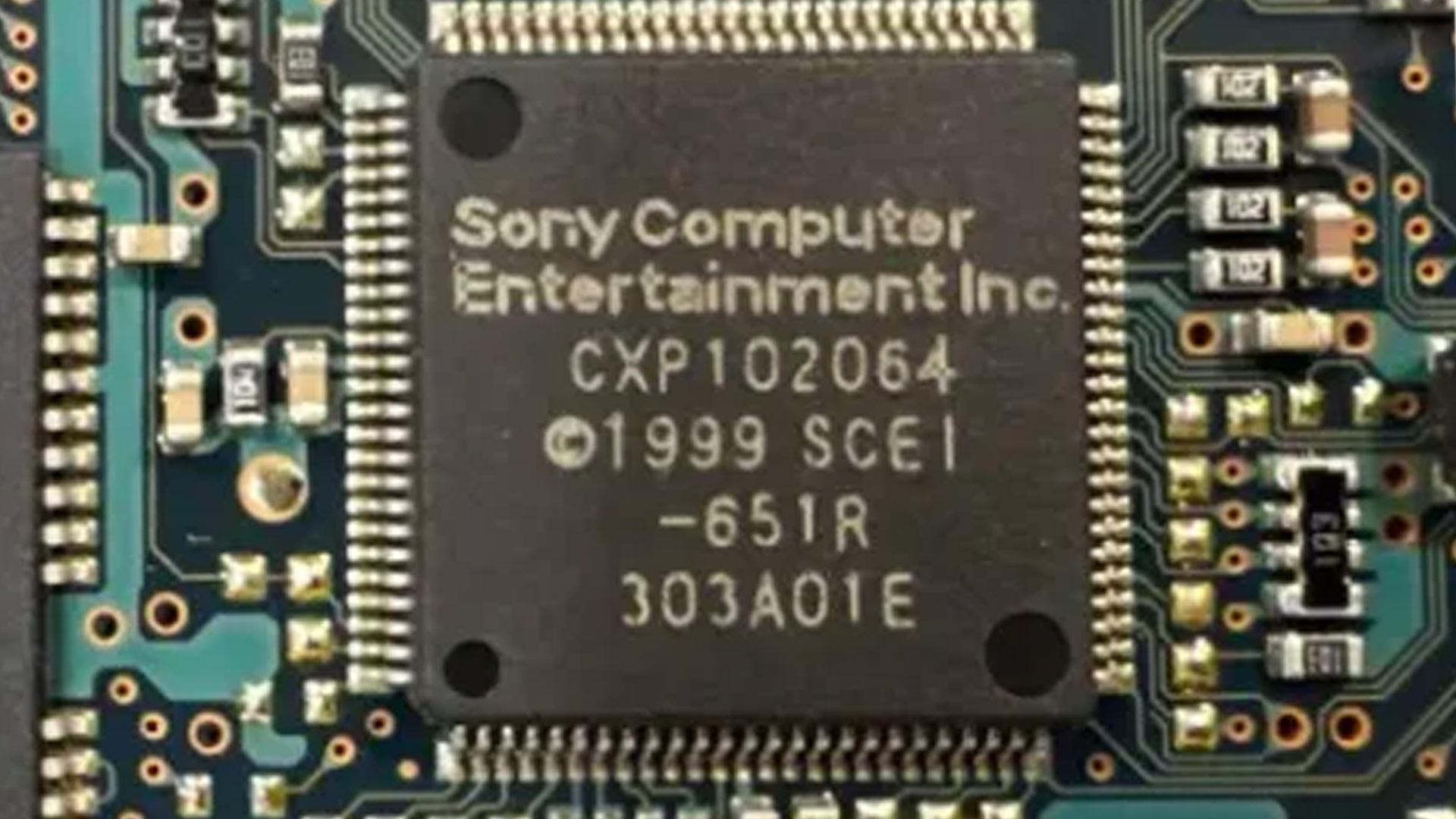
  23. Original Sony PlayStation 2 security chip 'broken wide open' after 26 years23
  24. A software thing I built: GPS on a 25MHz 486-SX24
  25. Show HN: I made a flight simulator, except you're just a passenger25
  26. The Google Play app review process now regularly takes longer than a week25
  27. Salesforce Global Outage25
  28. The DeepMind Institute25
  29. AWS says it can't restore some data from mideast facilities struck by Iran25
  30. Xiaomi Mimo 2.6 live post-training dashboard25
The Daily Front Page 2 of 26
Wednesday, September 16, 2026 The Daily Front No. #260916 — The Evidence Desk
article

Apple Reference Image: A New Approach for Verified Photography

by imwally·▲ 504 points·334 comments·security.apple.com ↗
prove that something actually happened

Today, powerful, widely available AI tools allow users to easily generate or alter photorealistic images to a degree that was difficult to imagine just a few years ago. These tools enable helpful features, like one-touch removal of background distractions, but they also make it difficult to distinguish between photographs that depict real events, and synthetic images that are heavily altered or entirely generated. So, in the case where the essential role of a photograph is to prove that something actually happened, an image appearing photorealistic is no longer sufficient to establish its veracity.

This is not a simple problem to address. Modern cameras rely on sophisticated image-processing algorithms to produce the final viewable image, so certifying that an image accurately reflects what a real camera sensor captured requires a chain of trust covering the sensor as well as the computational photography software that interpreted the capture. Industry approaches to this problem, based on the C2PA standard, attach provenance metadata after capture and certify the history of image edits from that point forward. This approach, however, is vulnerable to compromise at any point in the editing chain, and a viewer has no way to detect such a failure. It can also create privacy risks for photographers working in dangerous conditions by tying the image to a public identity, either to a particular device or to an individual.

iPhone is the world’s most popular camera and the most secure consumer mobile device, and as such Apple is uniquely positioned to take on this challenge. The iPhone camera is integrated into a platform that sets the industry’s highest standards of security from the silicon up. We also operate Private Cloud Compute (PCC), an industry-leading privacy-preserving cloud infrastructure that is secure, auditable, and can perform verifiable algorithmic operations without allowing anyone — even Apple — the ability to see the data being processed.

Leveraging these state-of-the-art capabilities, we have created Apple Reference Image, a novel solution for verifiable photography on iPhone, and debuting on the main camera sensor of iPhone 18 Pro and iPhone 18 Pro Max. This new, opt-in camera mode lets a photographer create a securely timestamped reference image that accurately reflects what was captured by the iPhone's camera sensor. Dedicated secure hardware on the device protects the integrity of this reference image, and Private Cloud Compute protects the privacy of the image data during processing. The system is built to be resilient to compromise, no matter how unlikely: any fraudulent images can be revoked without exposing the photographer's identity.

Apple Reference Image offers a trustworthy, scalable guarantee that a reference image is what it claims to be: a real photograph, captured by a real sensor in an iPhone camera, at a specific time. It sets a new standard for verifiable digital photography.

The Core Requirements of Apple Reference Image

A high-assurance photographic provenance system must meet three core requirements:

  • Semantic authenticity: a reference image must faithfully show what the sensor captured. Transformations of image data from the raw captured pixels to the final viewable image must be publicly verifiable.
  • Resilience to compromise: image authenticity cannot be undermined by tampering with the camera sensor, through common cryptographic attacks, or via software-level jailbreak of the device. If, despite these protections, any fraudulent reference images are created, they can be revoked.
  • Privacy preservation: an outside observer cannot determine whether any pair of reference images were taken by the same device. Image contents are not exposed to Apple or anyone else.

Apple Reference Image leverages custom-designed image sensors in iPhone 18 Pro and iPhone 18 Pro Max to ensure reliable capture of image data, and relies on Private Cloud Compute, which provides a computational environment for secure photographic processing that cannot be subverted even in the case of device compromise. We believe no other commercially-available photographic provenance system meets these strict requirements.

Semantic Authenticity

For any photographic authenticity system, the defining goal is that a user can trust that what is shown as the authenticated image corresponds to the scene that was actually photographed. A central challenge these systems face is how to secure the extensive photographic processing pipeline of a modern computational camera. Simply signing the raw values emitted by a sensor does not yield a viewable image: these pixels still need significant processing, like demosaicing and lens-shading correction, to be usable. To solve this, prior industry systems have delayed signing images until they reach the end of their software processing pipeline. But this approach is vulnerable to attacks that inject spoofed pixel data onto the data transport from the sensor, or to compromises of the device operating system that can completely alter the image before signing. Neither signing raw sensor values, nor delaying signing until the photograph is processed, meets our bar for semantic authenticity. Our solution hinges on splitting the Apple Reference Image process into two phases: creating a secure digital negative, and developing that negative into a reference image. Each phase receives our strongest protections.

The creation of a secure digital negative begins with a secure boot of the camera sensor into a specialized reference capture mode. The mode instructs the sensor to cryptographically sign pixel data immediately after capture, and prevents the sensor firmware from modifying the data. This creates a hardware-enforced assurance that the operating system receives pixel data exactly as the hardware sensor captured it, preventing injection or tampering attacks.

We treat image metadata with the same level of protection. Sensor-produced metadata is signed at capture time together with the pixel data. For the few metadata values that originate beyond the camera sensor, such as digital zoom boundaries and focal length, we use the Secure Enclave Processor (SEP) to sign the values. This off-sensor metadata cannot alter the pixel values themselves.

Knowing when a photograph was captured is often a critical element in establishing its veracity. While prior industry systems have included a timestamp provided by the general device operating system, we believe this plainly falls short of the real-world assurance need. Instead, Apple Reference Image provides both a lower bound and an upper bound on capture time from Apple’s cryptographic timestamp service, and we guarantee the photo was taken between the two bounds. On a regular heartbeat, the device requests a cryptographic timestamp token, and retains the most recent one it has received. Globally this happens on average every 15 minutes, though the interval depends on local network conditions. This provides a proven lower bound timestamp for the photographic capture. After capture, the device requests a second timestamp to use as an upper bound, and both timestamps are embedded and signed with the sensor data.

As a result, the secure digital negative contains all the essential information for rendering a reference image — the pixel data, essential sensor metadata, and the secure timestamp bounds — all protected from device software compromise.

To develop this secure digital negative into a user-visible reference image, we take advantage of the privacy-preserving computing environment provided by Private Cloud Compute. When the user chooses to create a reference image, the device uploads the digital negative to PCC, which runs the processing steps needed to render the image — including demosaicing, tone mapping, and compression — in a highly secure, private, and verifiable environment. Experts can verify that PCC doesn’t alter a digital negative during development: they can examine the software that does the work. Every production build of PCC is recorded in an append-only, cryptographically tamper-proof transparency log, the binaries are available for public inspection, and a device will only send data to a node that can attest to running a build from that log. These are the same extraordinary guarantees we make for how PCC protects the privacy of Apple Intelligence requests, which are described in depth in previous posts.

Apple Reference Image combines the strong guarantees of these two stages — the hardware-level assurance over the secure digital negative, and PCC’s verifiable transparency over the processing algorithms — to provide industry-leading semantic authenticity for the resulting images.

Resilience to Compromise

In designing Apple Reference Image, we considered a broad range of attacks, and constructed the system so as to resist compromise from multiple vectors.

As described above, we designed the core reference image pipeline to withstand a compromise of the operating system, or a data injection attack on the sensor bus. But we needed additional safeguards against a broader class of hardware attacks that could involve removing the sensor from the device.

These defenses begin before a single picture is taken, at manufacturing time. When the image sensor is first initialized in the factory, it creates a cryptographic signing identity, sharing only the public key with the factory. The SEP similarly creates a separately-attested signing identity. These identities are bound together into the device manifest, allowing us to later check whether a particular sensor and SEP are from the same device. At capture time, the device incorporates this platform information into the digital negative it produces. When the reference image is then developed in PCC, PCC can validate that the photograph has come from a valid sensor-device pairing.

We also considered cryptographic attacks. Existing photo signing schemes, to our knowledge, all sign with classically secure algorithms, but quantum-secure algorithms are increasingly critical to the long-term integrity of cryptographic signatures. Because reference images are published assets whose integrity must survive for as long as anyone might want to check them, a signature secure only against classical adversaries isn't sufficient: an image asserted to be authentic in 2026 should be securely verifiable in perpetuity. So we designed the system to resist quantum attacks on any algorithm used to protect the integrity of publicly distributed reference images. The final signature on a reference image is a composite post-quantum signature combining RSA-3072 and ML-DSA-87. To our knowledge, Apple Reference Image is the only image provenance system that provides quantum-secure defenses.

Finally, as no security system is perfect, we created a revocation system that can revoke individual photos, as well as all photos from a specific sensor. As part of developing the secure digital negative, PCC computes a confidence score that assesses whether the image has the physical characteristics expected of raw output from our camera sensors. Before the developed reference image is signed, PCC sends the photo GUID, sensor ID, and this confidence score to a companion service, which records them and updates the running score associated with that sensor. If a low-scoring sensor is revoked, PCC will no longer sign its images. Apple devices fetch updated revocation lists on a regular cadence; any time a reference image is viewed, the viewer can have confidence that the image isn’t known to be fraudulent.

Privacy Preservation

Other industry solutions require a photographer or institution to vouch for an image using their own credentials. We are concerned this puts some photographers, such as those operating in conflict zones, in a difficult position; it should not be necessary to forgo anonymity in order to prove image authenticity. We built Apple Reference Image to avoid using an explicit, public credential for photographers, and to avoid even implicit public association between different photos taken by the same sensor. The final reference image is instead signed by Apple’s signing service, after validation by PCC. That signature is backed by Apple’s strongest technical guarantees.

Our implementation also protects the confidentiality of the image itself, including from Apple. Merely capturing a reference image should never expose the actual pixels to Apple or anyone else. We achieve this through the exceptional privacy properties of PCC — the nodes themselves are architected so that not even Apple can access image data, just as Apple cannot see the information processed for Apple Intelligence in PCC. While the revocation service must maintain a private record of photo GUIDs and associated sensors to allow for revocation, it never has access to the image data, and does not allow for public access to this record. And as final revocation checks occur using on-device lists, a device never reveals to anyone which photo it's looking at in order to find out whether it's still valid.

Last, we have taken care to limit network visibility wherever possible. Timestamping requests travel over Oblivious HTTP, so the timestamp service never learns the IP address of the requesting device. Similarly, calls to the revocation and signing services occur from within PCC itself, which provides only the minimum information required for those services to function. Altogether, we believe these privacy protections are far stronger than in any existing image provenance system, allowing both photographers and viewers access to authentic images without inadvertently revealing their personal information.

Across all three requirements — semantic authenticity, resilience to compromise, and privacy preservation — we believe that Apple Reference Image sets a new standard for security in the industry. For readers who are additionally interested in the technical details of our implementation, the next section will describe the precise manufacturing, signing, and verification sequences that underpin the security guarantees of Apple Reference Image.

Technical Details

Reference Image Set-Up

The foundation for Apple Reference Image is created during device manufacturing. When an Apple photo sensor is first initialized, it generates its own ECDSA P-256 signing key pair and never releases the private half. The factory recording station retrieves only the corresponding public verification key, signs it with a factory certificate authority (CA), and records the key and certificate in the device's hardware manifest.

The Secure Enclave Processor (SEP) goes through a similar process: it generates a key certified by our Basic Attestation Authority (BAA) under a separate CA, which lets the device later produce signatures that Apple can attribute to that specific phone. A third CA then signs the device manifest itself, binding the sensor key and the BAA-attested SEP key together as belonging to the same iPhone. This binding is what later lets us state that a particular sensor and a particular Secure Enclave were, and are, part of the same device.

Once the device is in use, it begins timestamp collection. Apple Push Notification Service (APNs) runs an existing heartbeat protocol to ensure the health of the connection for push notifications. Coinciding with this heartbeat, APNs now delivers an up-to-date RFC 3161 timestamp token from Apple's timestamp service, signed with ECDSA P-256 over SHA-256, and the device keeps the most recent one it receives.

Image Capture

To begin the capture process, the user switches to Reference mode. This reboots the sensor into the specialized, secure reference mode. This capture mode accepts one input from the device operating system: a SHA-256 digest to be embedded at a fixed location in the captured frame’s metadata. The digest is computed from the most recent secure timestamp, the device manifest, and the device's secure boot manifest.

At capture, the sensor measures light as an analog signal, which is digitized. The digitized frame and the embedded metadata digest are signed together, inside the sensor, with the sensor's private key. OS-derived metadata (digital zoom factor, exposure, and lens parameters) is collected from the camera system. We take a commitment to the sensor's signature together with this metadata and sign it with the SEP, using the BAA-attested key.

We compute a SHA-256 commitment to the SEP signature and send it to the timestamp service, which returns a signed token establishing that the photo existed no later than that moment, an upper bound to complement the lower bound already embedded in the frame. If the device is offline, no upper bound is available yet; a background process keeps attempting the request and inserts the token once it succeeds, producing the tightest interval the circumstances allow.

Everything produced so far — the pixels, both signatures, the timestamps, the metadata, the device manifest, and the secure boot manifest — is stored in the secure digital negative on the device, in DNG format, linked to the conventionally processed photo from the standard pipeline. The negative can sit there indefinitely, and it can also be shared in this undeveloped state, a workflow professional photographers may need.

Reference Image Development

When the user initiates developing a reference image, the device uploads the secure digital negative to Private Cloud Compute. PCC recomputes the digest embedded in the frame and verifies the sensor's signature over the pixels and that digest, verifying the certificate chain back to the sensor CA. PCC also verifies the SEP signature and chains it to the BAA CA, and it verifies the signature on the device manifest and chains it to the CA that signs device manifests at the factory. It then confirms that the sensor and SEP named in those chains belong to the same device. Only if all these checks pass does processing continue.

PCC next checks the timestamps. If the lower-bound timestamp fails verification, PCC substitutes March 31, 2026, since the feature didn't exist before that date and no photo can predate it. If the upper-bound timestamp is missing or doesn't verify, PCC substitutes the current development time in PCC.

Using a neural network with hidden weights, PCC computes a confidence score for the photograph. This additional step confirms that the image has the physical characteristics expected of raw output from our sensors, increasing confidence in its authenticity. PCC then develops the negative with demosaicing, tone mapping, and related corrections. The result is compressed as a JPEG and hashed, creating a commitment to the developed image. This hash serves two purposes: it's the value that will be signed, assuming it passes our remaining checks, and it supplies the bits used for the photo GUID.

PCC sends the photo GUID, the raw hash, the confidence score, and the sensor ID to a companion service, which records them, updates the running confidence score associated with that sensor, and confirms the sensor doesn't appear on a revocation list. If these checks pass, PCC then submits the commitment to our signing service, which signs it with a composite post-quantum signature using a hybrid MLDSA87-RSA-3072-PSS-SHA512 scheme. The signature is embedded in the JPEG, and the reference image is returned to the device, which associates it with the main photo from the original capture.

After the secure digital negative is successfully developed, it's automatically moved to the deleted photos folder. As with any deleted photo, the user can recover the negative for preservation if desired, or delete it immediately; otherwise it's automatically purged after 30 days.

On the client side, whenever the reference image is displayed, the client verifies the final signature on the JPEG and confirms its photo GUID doesn't appear on the current revocation list before showing the image.

Conclusion

Apple Reference Image builds on Apple's unique foundation of capabilities in hardware and software, including sensor identity certification at the factory, silicon security, and Private Cloud Compute, giving photographers a new way to provide a verifiable photograph. This allows them to attest to what their iPhone actually captured, without requiring them to expose a public identity or place trust in a third party. At its core, Apple Reference Image binds a signature from an iPhone camera sensor to a securely timestamped, tamper-evident record, developing it inside PCC while running publicly verifiable code, and signing it with a composite post-quantum signature designed to remain secure for decades. If a device is later found to be compromised, its images can be revoked and flagged retroactively, without revealing which images came from the same sensor. The result is a verification model that offers photographers, newsrooms, and everyday users renewed confidence that an image they’re viewing is a photograph actually captured by a camera.

The Daily Front Page 3 of 26
Wednesday, September 16, 2026 The Daily Front No. #260916 — The Watching Machine
article

Hackers Got Inside a Flock Camera

by driverdan·▲ 494 points·231 comments·wired.com ↗
the device captured 1.6 million images of 50,000 vehicles in 21 days

A hacker collective pulled down a Flock camera and dumped its data. The files included thousands of videos and logs showing that the device captured 1.6 million images of 50,000 vehicles in 21 days.

Hackers Got Inside a Flock Camera. Its Data Shows How the System Really Works

Photo-Illustration: Jobanny Cabrera; Getty Images

Hackers ripped down a Flock camera above a roadway, made a near-complete copy of the data stored inside it, and shared the files with 404 Media and WIRED, revealing in new detail how exactly Flock Safety’s cameras track the movements of both vehicles and people. The hackers say they are also publishing details on how they managed to obtain the software, in the hopes that other people may copy them.

The breach provides an unprecedented look inside a system that Flock has described as protected by on-device encryption. The hackers were able to copy the camera’s storage and recover an encryption key stored on the device, which unlocked videos of thousands of vehicle detections. The hackers shared the material with 404 Media and the transparency nonprofit Distributed Denial of Secrets, which shared the data with WIRED. 404 Media and WIRED then analyzed those files as part of a joint investigation.

While much of the automatic license plate reader’s most sensitive storage remained encrypted and inaccessible, the joint analysis of the recovered data shows that software running on the device explicitly detects people as well as vehicles, license plates, and bicycles. The camera can produce dozens of images of a single passing vehicle and, according to several weeks of recovered logs, generated more than a million images. Its computer-vision software also sometimes isolated bumper stickers and other graphics, including, in one case, an American flag patch on a motorcyclist’s saddlebag.

The act of removing the camera and dumping its software shows that some people are not content with just destroying or removing the cameras. Across the country, multiple people have been arrested for allegedly tampering with or otherwise sabotaging Flock’s cameras. In response, some towns have announced that they are going to stop using Flock’s cameras altogether, and in one case, a police department even made a fake, 3D-printed Flock camera case in order to bait potential vandals.

“Why just destroy them when we can reverse engineer them and find the secrets of those spying on us?” one of the hackers, from a collective calling itself stegan0gram, said in an interview. “We liberated hardware in the field, disarmed them, and proceeded with reverse engineering of the cameras and associated solar equipment.”

Flock’s cameras photograph passing vehicles and send the images and other data to the company’s servers. There, Flock’s system presumably reads the license plate and can identify characteristics such as the vehicle’s color, make, and model. Flock then makes these time-stamped records searchable by whichever local agency owns or has access to the cameras. But in many cases, Flock’s system also allows other police departments from all over the country to search those cameras too, as part of the company’s national network. In Alpharetta, Georgia, for example, WIRED found that records from the city’s Flock cameras were accessible to more than 2,000 agencies, including police departments, colleges, airports, and, inexplicably, the Office of Inspector General for the federal General Services Administration.

This national network has been a selling point for Flock but also a deep source of controversy. 404 Media revealed that local cops were performing lookups in the national network on behalf of Immigration and Customs Enforcement, including in areas that banned working with immigration authorities or transferring license plate data out of state. 404 Media also revealed that a cop in Texas searched Flock cameras nationwide for a woman who self-administered an abortion. Those stories, among others, triggered a national conversation about whether people want Flock cameras, or automatic license plate readers more generally, in their communities.

And in the case of stegan0gram, the answer is clearly no.

The hackers said they were able to access the Android system on the camera and found two partitions—sections of its hard drive, essentially. A few of these were unencrypted, the hackers said, including one called “vendor” and another called “media.” The latter contained an encryption key that unlocked another part, which contained much of the media—the videos and stills—the camera took.

In early 2025, security researcher Jon “GainSec” Gaines reverse engineered a Flock license-plate reader and documented flaws that could be used to gain root-level access. After Gaines disclosed his findings, the company acknowledged the findings but downplayed their severity, writing that the flaws required physical access to the device and that even someone who gained access to a camera “would still not be able to gain access to footage,” because images remained on the device only briefly after being transmitted to the cloud.

404 Media and WIRED analyzed the camera’s contents. The device’s processor is similar to those used in midrange smartphones, and it runs about 20 Flock-built apps that handle everything from detecting motion and taking pictures to classifying objects, uploading data, and receiving remote updates.

According to the code, when something moves into view, the camera takes a rapid series of photos. A typical passing vehicle generated about 28 images, though some produced more than 100. The camera uses different exposures to capture both the license plate and the wider scene, then scans the images, selects and crops useful frames, and sends them with other data to Flock over the cellular network. The camera itself does not appear to read the plate or identify the vehicle’s make, model, and color. That appears to happen on Flock’s servers.

According to our analysis, the camera’s logs recorded about 21 days of activity across several periods. During those windows, the device photographed roughly 50,200 vehicles and generated about 1.6 million images. On a typical day, it logged around 3,300 vehicles, with a high of 4,454. Those figures would vary considerably depending on where a camera is installed and how much traffic passes in front of it. The camera was almost certainly operating outside those periods, but older logs had been overwritten or were no longer recoverable from the device.

The software running on the camera explicitly detects people, something which is typically overlooked in discussions around Flock cameras. When it spots a person, it records where they appear in the image and how confident it is in the detection.

To test what the software could actually see, WIRED extracted the models from the camera’s files and ran them against test images and footage recovered from the device. The models readily detected people, including a selfie of a reporter. WIRED then ran them across 27,321 short videoclips stored on the camera. The clips were MP4 files, each about one to two seconds long, recorded at 1,024 by 768 pixels without audio. They were separate from the rapid bursts of higher-resolution still images the camera also takes as vehicles pass. The models detected people in 11 of the clips, all of them riding motorcycles. The small number is likely due to the camera’s position above a roadway, pointed down at passing traffic where pedestrians were unlikely to appear.

The tests also showed how broadly the camera’s license plate detector could interpret what it saw. In some cases it mistook bumper stickers, dealership frames, and other graphics for license plates and cropped them out as if they were plates. In one video of a passing motorcycle, the detector cropped an American flag patch on the rider’s saddlebag as if it were a plate.

Flock insists its cameras do not perform face recognition. WIRED and 404 Media found no evidence of any face-recognition capabilities in the camera’s software beyond ones included by default in the Android operating system. Those capabilities did not appear to be enabled or in active use.

In August, WIRED obtained frontend code for Flock’s police software, now called OS Investigate and previously known as Nightshift, and reconstructed portions of the tool. That software showed how Flock can use the records generated by its cameras, along with police files and commercial data, to identify drivers, surface vehicles that repeatedly travel together, and search for people based on patterns of movement. The data provides a view of the other end of a system.

A Flock spokesperson said in a statement: “The unauthorized removal and tampering of a Flock camera is illegal.” When asked specifically about the encryption key stored on the camera, the company added, “Flock takes security seriously and maintains a public Vulnerability Disclosure Policy for security researchers to report potential vulnerabilities directly to us. We received no report through that process, and based on the limited information provided, we do not have enough detail to assess the claims being made. If the individuals identified legitimate vulnerabilities, we encourage them to submit their technical findings through our vulnerability reporting process so our security team can review them and take any appropriate action.”

One of the hackers said, “Being investigated is a legit concern and something we are trying to avoid. I'm sure our actions have attracted some attention as it is, but we are careful and try to keep a low profile.”

Noel Pichardo, a former Pawtucket, Rhode Island, police officer who became an outspoken critic of Flock after challenging his department’s use of the cameras, says he understands the activists’ frustration but worries that sabotaging devices could ultimately strengthen the case for them. “I think that type of vigilantism will only crystallize the police and the state at large in their belief that this tool is necessary,” Pichardo says. “The longer the state continues to ignore the groanings of their constituents who are against this type of surveillance, the more this will happen.”

The camera’s logs also show the camera struggling with storage. Its logs recorded more than 27,000 “no space left on device” errors while trying to save full-resolution images, along with tens of thousands of related errors, crashes, and reboots. At the same time, about every two minutes, code checked that the camera was still running and logged the message, “Who’s a good boy?!” More than 12,000 of those messages appear in the recovered logs.

When the camera did restart, another service left a final message in the logs: “A reboot was requested! ¡Adiós, Amigos!”

The Daily Front Page 4 of 26
Wednesday, September 16, 2026 The Daily Front No. #260916 — Allies at the Door
article

EU chief opens door for Canada to become 'associate member'

by hackernj·▲ 653 points·831 comments·bbc.com ↗
opening the door

EPA A smiling Mark Carney, wearing a suit, walks alongside European Parliament President Roberta Metsola and Ursula von der Leyen at the European Parliament

Mark Carney (left) walks alongside European Parliament President Roberta Metsola (centre) and European Commission President Ursula von der Leyen (right)

The president of the European Commission has backed proposals for Canada to become the EU's first "associate member".

Ursula von der Leyen told the European Parliament on Wednesday she wanted to work on "opening the door" for Canada, which would involve closer ties on various key sectors.

The country currently faces tense relations with the US, compounded by an intensifying dispute over trade.

Insisting it would not be a "partnership against anyone else", Von der Leyen did not mention Donald Trump by name. Nevertheless the US president threatened to cut trade with the European Union in response to the proposal.

Canadian Prime Minister Mark Carney last week spoke of seeking a "unique alliance" with the EU.

Carney was in attendance at the annual key note speech in Strasbourg, and is due to address the parliament on Thursday.

Trade talks between Canada and the US collapsed last month, sparking a series of new tariff measures. Trump's repeated talk of making Canada a "51st state" has also helped to fuel the feud between the North American neighbours.

Von der Leyen told the EU's State of the Union address that the bloc and Canada "see the world with the same eyes", including on topics ranging from AI, to climate change and geopolitics.

"And we have stood together: on Ukraine, on defence, on raw materials and on supply chains. But above all... Europe and Canada believe in democracy."

She added: "Partnerships are a strategic choice for Europe. But they also respond to the fracture in the international rules-based system".

She did not give specific details on how any Canadian membership would work, but listed manufacturing, technology, artificial intelligence (AI), defence, energy, critical minerals and economic security as key areas for cooperation.

When asked about the plan, Trump called it "laughable".

"If they do that, if I think it's at all a hostile act, I will put very serious tariffs or stop trading with Europe, on many things."

He added: "If it's a good intention, that's fine. If it's a bad intention, we'll put very heavy tariffs on Europe, which is a possibility."

Both von der Leyen and other European leaders have found a reliable ally in Carney as they deal with similar problems.

In particular, they have faced Trump's aggressive use of tariffs and his threat to annex Greenland which is a sovereign territory of EU member Denmark.

But "associate membership" of the EU does not currently exist and the process, if agreed, could take years.

Earlier this year, Germany's Chancellor Friedrich Merz suggested - to a mixed reaction - that Ukraine could be granted this new status.

Some countries in the western Balkans including Albania, Bosnia and Herzegovina, Montenegro, North Macedonia, and Serbia are already on the long road towards full EU membership.

In Eastern Europe, Georgia and Moldova are also applying.

Ten of the bloc's 27 members are yet to ratify a free-trade agreement struck with Ottawa nearly a decade ago, and some capitals would prefer to build on existing defence and trade agreements rather than create a new form of membership for Canada.

EPA Ursula von der Leyen, who has a grey/blonde short haircut, wears a cream blazer and blouse as she speaks at a podium, with the EU flag in the background

Von der Leyen said it was time to bring the EU's relationship with Canada to "the highest level possible"

Setting out the EU's political and policy priorities for the year ahead, von der Leyen also proposed the formation of a European Security Council, which would include the UK and Ukraine, amid an ongoing threat to the continent from Russia.

"For a long time, we have discussed a leaders' format focused on the security of our continent, with partners like Canada, Norway, Ukraine, the United Kingdom and others involved," she said in the wide-ranging address.

"This is even more urgent now, given the nature and scale of the risks at play. This is why we will set out our ideas to make a European Security Council a reality."

Calls for such a body have been growing since Russia's full-scale invasion of Ukraine in 2022.

It was initially a French-German conception but more countries have shown support, particularly as Trump has questioned the Nato military alliance. Other nations worry such a council could unhelpfully rival Nato.

Von der Leyen said the EU was "strengthening our work with Nato" and that expanded defence spending would be "fully aligned" with the alliance.

But at the core of such a security council would be the ability to trigger an emergency meeting if one member felt under threat, similar to Nato's Article 4.

The EU chief said it would be a "mechanism to flank" Article 4, a term that could be interpreted as complementing Nato functions or - if taken in a military context - bypassing them.

Alongside global threats, von der Leyen also said many European families were worried about the cost of living, and the "dizzying speed of change" of technology and its impacts on jobs and society.

Other proposals included inviting the world's largest AI labs for talks on how to support industry efforts to pace the frontier, as well as slashing bureaucracy for businesses in the EU.

Plans to curb social media use among children, including banning platforms for under 13s, were also put forward. Under the proposal, children aged 13 to 15 would only be able to set up social media accounts which are supervised by parents.

A new emergency tool to help countries better deal with mass migration movements following the deadly influx of migrants to the Spanish enclave of Ceuta in July would also be outlined.

The pledge chimes with the message of European politicians on the right and hard right who have gained support in recent years for proposing a tougher approach.

Some of them called the mass attempt to enter the EU through Ceuta an "invasion" and argued asylum rules should be suspended to deal with such a crisis.

Von der Leyen said the new emergency tool would "only be triggered under a strictly defined set of criteria" and for a specific period of time, and that fundamental rights would be protected.

Human rights groups worry such a move would see vulnerable people, including women and children, turned back and denied the protection afforded to them under international law.

The Daily Front Page 5 of 26
Wednesday, September 16, 2026 The Daily Front No. #260916 — Driver, Prompted
article

Building a Linux GPU Driver for the M4 Mac Mini in One Month

by ADevWithAnIdea·▲ 411 points·267 comments·codyho.dev ↗
a process which normally takes years

What We Did

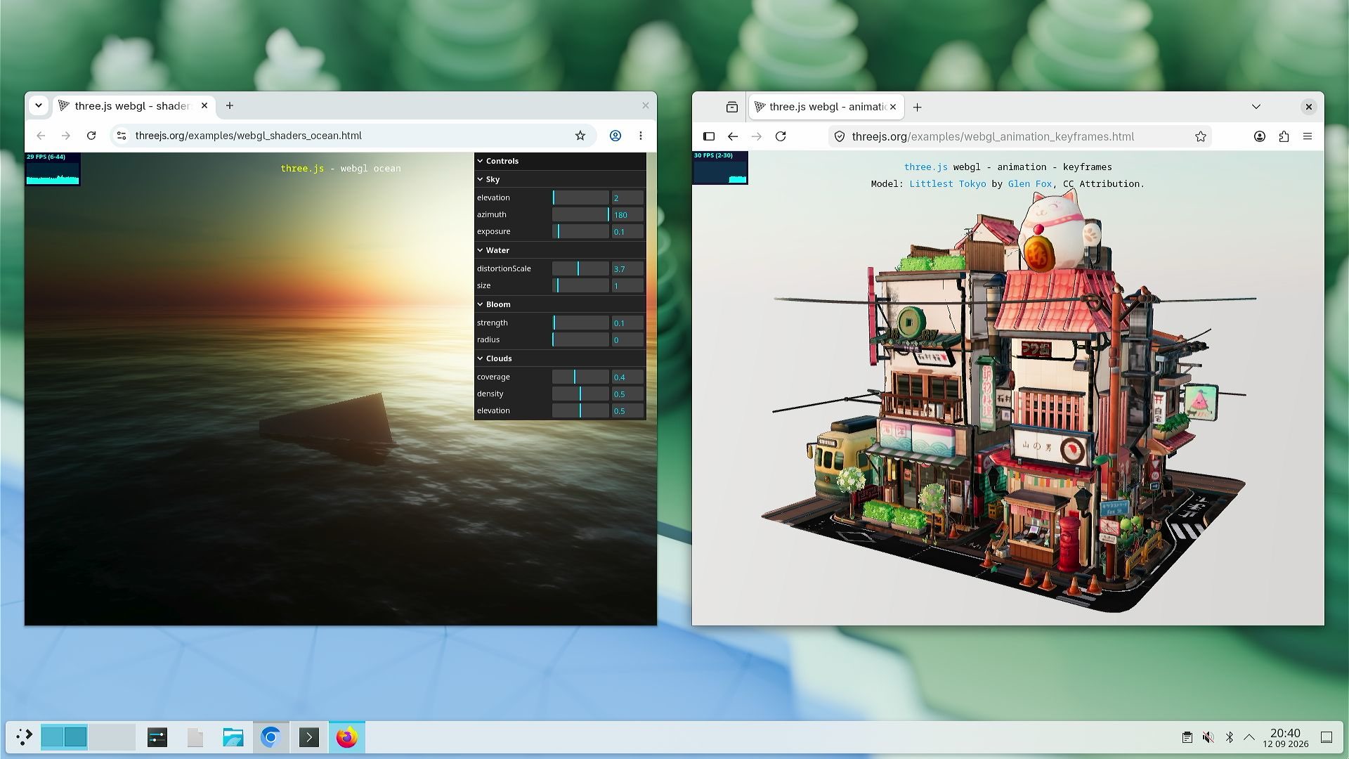
TL;DR: Niklas and I built a fully OpenGL ES 3.0 compliant GPU driver for the M4 Mac Mini and MacBook Neo in about a month, a process which normally takes years. Here is Chrome and Firefox running WebGL on the M4 Mac Mini with working compositing:

Chrome and Firefox running three.js WebGL demos on our driver.

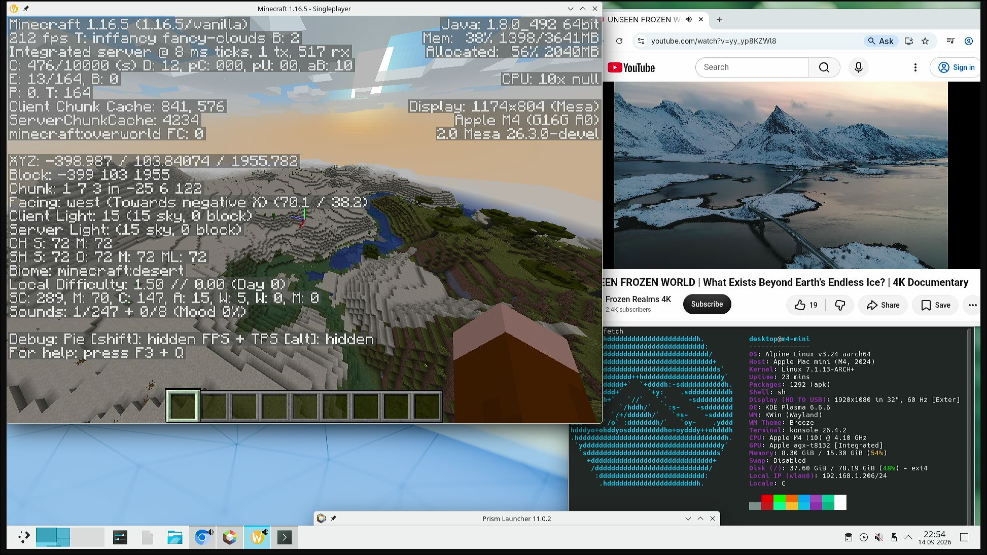
Most importantly, the driver is fast enough to run Minecraft at 200fps:

Minecraft running at 212fps on the M4 Mac Mini.

Building this driver involved reverse engineering the AGX’s (Apple’s name for the GPU) incredibly complicated firmware ABI and user-space components. This was all done in a transparent, verifiably clean room manner using well established techniques. The code is not yet ready for end users, but we are looking to get it to end users as soon as possible.

How We Did It

Previously, I built a hypervisor to reverse engineer macOS. Now the goal became to actually do something useful with it, and what better target than writing a GPU driver. The GPU is effectively a requirement for any modern system, otherwise everything needs to be CPU rendered which is orders of magnitude slower and less power efficient. Our goal was to implement conformant OpenGL (and soon, Vulkan) drivers for the M4 Mac Mini and MacBook Neo.

Normally, building a GPU driver is an endeavor that takes years; our goal was to do it in days. It turns out that days was overly optimistic, but weeks is still a massive improvement. In those weeks we have:

  • Reverse engineered the M4, A18 Pro, and (mostly) M5 user space using only live probing, discovering hardware-supported features and instructions not emitted by Apple’s driver
  • Built a fully working user-space driver, including a new custom IR/shader compiler, command stream builder, and many more components
  • Reverse engineered, from scratch, the full AGX firmware ABI using traces from the hypervisor I previously built
  • Implemented a full Linux kernel driver for said firmware ABI

Throughout this process, we have not looked at any Apple binaries, only hardware traces (from our hypervisor) and shaders we built ourselves. For user-space graphics RE, we were careful to treat any required Apple blobs as opaque objects. We had a friend write documentation on these blobs 1 so we could write a clean room implementation ourselves (which was mostly built by just blindly trying stuff until it worked). We have published all of our experiments so that anyone can verify the provenance of our work (see the twin agx-re repos under Deliverables).

This blog post is divided into two parts, user and kernel space. This mirrors the split in all modern GPU drivers: the kernel is responsible for interfacing with the firmware, allocating buffers, and managing scheduling, while the actual contents of those buffers and what is being scheduled are opaque. User space is responsible for actually understanding how the GPU works and filling those buffers with stuff.

Kernel Space

On Apple Silicon, the kernel driver does not interface directly with the hardware. Instead, it talks to the GPU firmware running a custom RTOS called RTKit. That means that the first step to a kernel driver is not talking to hardware, it’s figuring out the firmware ABI.

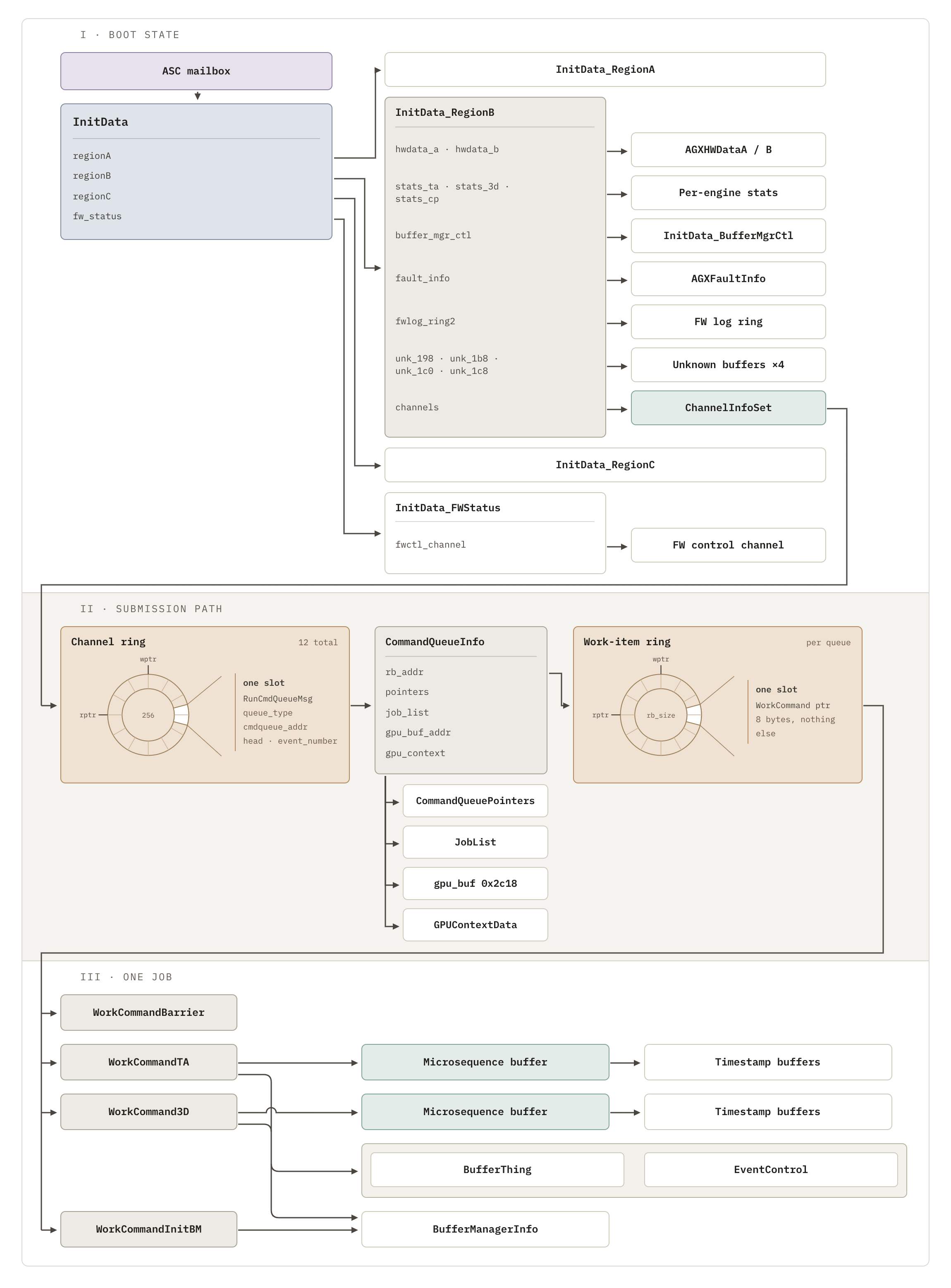
The firmware ABI was by far the most annoying part of this project, because rather than doing the sane thing of coming up with a reasonable ABI with nice interfaces, Apple essentially took a regular kernel driver, cut it in half, and then put half of it in the AGX and called it firmware, with the other half of the kernel driver communicating using shared structs in memory. Many of these structs have firmware owned fields (which we must never modify and which we must learn from reverse engineering) interleaved with host controlled fields. For an idea of how complicated the ABI is, this is what the shared memory tree looks like on the M1/M2:

The M1/M2 firmware ABI

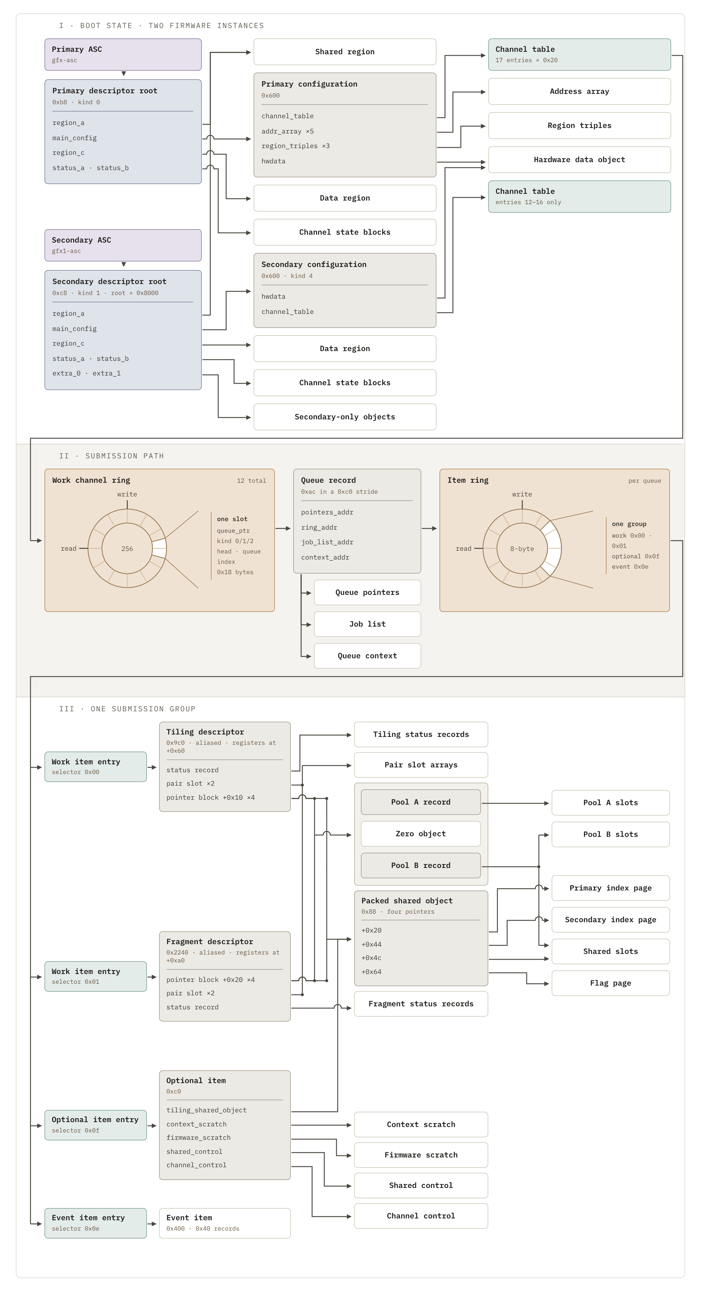
Asahi Lina famously figured all of this out over grueling 12-hour days to build the M1/M2 kernel driver, an amazing technical accomplishment. Unfortunately, the A18 Pro firmware ABI (I started my RE work on the MacBook Neo and later pivoted to the M4 Mac Mini) is significantly more complicated than the already very complicated M1 firmware ABI:

The A18 Pro firmware ABI

What the F@!#, Apple. Note how the A18 has:

  • 1.5x as many structs
  • twice as many pointers
  • a significantly more complicated process for submitting work

There are many other issues that add friction to the RE process 2. I did have some documentation on the firmware ABI, but it was highly incomplete and honestly was not very useful 3.

My approach was simple and based on the approach used to successfully reverse engineer the M1/M2 machines: watch what macOS did, replay it, then try to do it ourselves, which is made possible by the hypervisor.

When I described this approach to the LLM, it took replay extremely literally: the first thing it did was wait for the first firmware visible event (these are called “kicks”), then saved a copy of the entire GPU memory state. After a reboot, it copied the saved memory state straight back into host memory, performed the kick, and saw the output pages change. It would then try to reconstruct these objects in code, following all the pointers and making sense of the contents. Over successive experiments, Codex would reduce the number of pages it copied until there was no more replayed state and everything was built from source. 4 Amazingly, I noticed Codex had good taste regarding when it should poke the hardware some more and when it should just run the hypervisor and capture the state itself.

There were three major issues, and all were caused by our inability to get a clean capture of host work:

The first issue was render work submitted after the GPU firmware started. We could prestage work before the firmware started, start the GPU, and that work would be completed as expected, but once the firmware started any work submitted would just be ACKed and retired without actually doing anything. Once the firmware has started, capturing state is much harder because everything becomes dynamic and the firmware becomes a stateful object with state you can’t easily replay.

I had to step in at this point and examine Codex’s process. It turns out it was trying to replay a capture very late in the AGX’s lifecycle, where there had already been many previous events. When I told it to choose a capture far earlier in the AGX’s lifecycle, the very first capture after firmware start, Codex was able to almost immediately discover the issue (it was missing a single byte descriptor). This took a few days.

The second, and only major blocking, issue was compute. The AGX, broadly, supports two kinds of work: compute and render. In the regular GUI path, compute work is only scheduled after a significant amount of render work was already executed. Thus, it took a long time to get a clean capture of a compute workload, and when Codex finally did it was 336 MB and impossible to replay (it tried, for a long time). It also tried to construct the objects itself by looking at the capture, and spent over a week doing this, but was ultimately unsuccessful. There was just too much nonsense to sift through. This was exacerbated by issues on my side– after getting render working, I expected that submitting compute work would be simpler (the firmware ABI for compute is indeed simpler, so I was correct here), but lost my humility and thought it would be a cakewalk that would only take a few hours. Thus, I didn’t scaffold out the task properly for the LLM.

The fix actually was given to me in another Codex session. In essence:

  1. Disable the GUI by booting into single-user mode; this means no render work would be done.
  2. Install a LaunchDaemon to run at the earliest possible point, the moment Metal (Apple’s proprietary graphics framework) became available.
  3. Run a tiny Metal program that we supplied
  4. Capture and replay this tiny, pure compute trace.

The trace was captured successfully. Within a few hours, Codex had deconstructed it, and within a few days, Codex had compute working. As for why the original compute codebase didn’t work… Codex has no idea. The working one and the broken one look very similar.

In hindsight, this should have been the strategy from the start– smallest possible capture, run in single-user mode so as not to perturb results. I learned from my mistakes here for the final issue:

Partial renders ended up being one of the hardest things to figure out. They occur when the Tiled Vertex Buffer (TVB) isn’t large enough to store the current geometry (ie, there’s just too many triangles to draw). In these cases, there are two options, and the driver needs to support both: either increase the size of the TVB, or perform a partial render, ie, render part of the geometry, then reload the buffer with the rest of the triangles, and finish the partial render. These partial renders turned out to be very, very finicky, even more so than the rest of the work because they essentially mean adding save and resume to the GPU driver.

The workflow I discovered earlier came in very handy here. Codex was able to replay one partial render transaction, and then modified our Metal shader to perform multiple partial renders (this is pretty easy by just hammering a single tile with thousands of triangles until a partial render is triggered) and then learned how to replay these. Once Codex had a successful replay, it was only a matter of time until it learned how to build it ourselves.

Building the Kernel Driver

Moving from a Python prototype driver to a fully featured Linux driver took three days, and one of those days was almost totally wasted because Codex, for some reason I still do not understand, chose to tackle partial renders first (by far the hardest task) instead of doing compute first (the easiest task). Once I told it to do compute first, everything went smoothly.

At all high level, the entire process was, basically:

  1. Rewrite the existing drm-shim in Rust following the exact same pattern; this gives us a synchronous Rust driver.
  2. Rewrite the frontend to be asynchronous; the actual GPU submission remains synchronous.
  3. Refactor the GPU submissions to be asynchronous and, instead of polling, listen for firmware events and associate work with a fence
  4. Implement some low-hanging optimizations, such as batched work submission.

This is all pretty routine engineering work that LLMs are definitely capable of.

The only notable thing I found is that Codex aggressively used the hypervisor to debug why its code didn’t work, including capturing the full address space and comparing it to known good samples. This sort of systematic debugging is why Codex is by far my favorite coding agent.

User Space

The A18 Pro user space is very different from the M1/M2; it has new descriptor formats, a new ISA, and a bunch of other new things. Aside from being a tile based deferred renderer designed to run Metal, it’s just a different GPU.

The good news is user-space RE has a very well defined process. Simply write a small Metal program, compile it, run it, see what changed, then take it apart and start fiddling with the bits until we understand what all of them do. If you’re thinking this sounds like the sort of boring, repetitive, rote work that LLMs are very good at, you would be correct.

The RE work occurred in two phases. For the first phase, I had Claude look at every possible Metal program it could find and trying to build a disassembler, assembler, and understand the format of all the other descriptors/command streams/etc required for the GPU driver. I had Claude enumerate everything, including stuff Linux can’t use (like tessellation) for completeness. This was successful, but just because Claude could disassemble and then reassemble programs doesn’t mean it knew how to build one itself. When trying to close this gap, ie, understand every instruction enough to actually be able to compile our own arbitrary programs, Claude did a horrible job and made basically zero progress.

At this point, Niklas finished his drm-shim for the M4 Mac Mini and joined me for the second phase of user-space RE. We had two different approaches to actually finishing the user-space driver:

My approach was to prioritize hardware RE, and focus on just figuring out how the hardware and all the instructions worked. Then I would write a spec and let the LLM implement it, hopefully ending with full OpenGL and Vulkan compliance. This means that most of my LLM’s time was spent writing experiments on hardware, not actually implementing Mesa code. The idea was that once I understood the hardware, everything else followed.

Niklas took a different approach, that I’d describe as “Mesa first”. Essentially, he tried to build out Mesa first and would only do RE in order to build out some functionality. His time was split between building and testing Mesa, and performing RE.

It turns out that Niklas made significantly faster progress than I did, because my agent would spend a lot of time on minor, inconsequential tasks in the name of completeness. By contrast, his agent was grounded by the need to actually build Mesa, so it used time and resources a lot more effectively. He ended up moving so much faster than me that ended up just trying to support his work by investigating any behavior he didn’t yet understand.

This was one big limitation of Codex I noticed. The best word I can think of to describe it is “pedantic”– it is extremely thorough all the time, which can be a major benefit in some scenarios, but other times it gets stuck in the weeds on some random tangent to the detriment of the overall goal.

During our RE, we found behavior that was supported by the hardware but not supported by Metal; this was found by directly messing with the bits of the different instructions and extrapolating what might exist based off what we know did exist, just like Alyssa Rosenzweig did when REing the M1/M2. This included:

  • A native single-instruction 64-bit add
  • Anisotropy to 128x (Metal caps at 16x)
  • A new mode of the matrix unit
  • 7-bit immediate support for uniform_mov

Mesa Development

There are a few things that massively work in our favor when building out user-space graphics. Most notably, the Khronos compatibility test suite (CTS) is already an exhaustive corpus of tests our driver must pass. In other words, the hardest and most sensitive part of working with LLMs, giving them good tests to ground them, is already done for us.

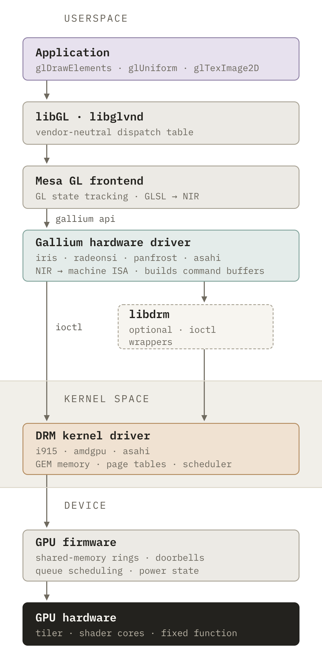
Additionally, Mesa already has great abstractions that make our lives significantly easier. This is what the modern OpenGL stack on Linux looks like:

Diagram of the modern Linux graphics stack.

All we have to do is translate between Gallium, Mesa’s internal API, and AGX hardware semantics. One of the biggest parts of this process is translating from NIR, Mesa’s internal IR that’s quite similar to LLVM IR, to the AGX’s proprietary ISA. As a bonus, this compiler can be reused for a future Vulkan driver.

Niklas was able to slowly iterate through OpenGL features, REing the user space as he went, until he finally achieved full OpenGL ES 3.0 compliance (the unsupported tests are optional extensions):

The OpenGL ES 3.0 conformance test suite passing on our driver.

Throughout the process, we benefited from the existing M1/M2 work: while the exact hardware semantics differ, the overall shape remains similar and thus many of the right tradeoffs/decisions were already made for us. Throughout my time building this driver, it became clear that Alyssa Rosenzweig and the others who built the M1/M2 driver are utter wizards– hats off to them!

Deliverables

Mesa: https://github.com/niklassheth/mesa

Linux Kernel Driver: https://github.com/GravityLinux/linux/gravity-m4

User-Space RE Documentation (horrible pile of LLM slop, but functional): Cody Niklas

Remaining Work

Vulkan 1.4, OpenGL 4.6, OpenGL ES 3.2, OpenCL 3.1, Direct3D 12 (via Proton), and ray tracing are all in scope. We want our driver to be as good as the best graphics drivers in the world.

Additionally, Niklas and I want to upstream all of this, but there are some significant obstacles. We used the unmodified Asahi UAPI, so there are no policy issues with Mesa upstreaming, but it needs far more testing, human review, and to be refactored into a reviewable PR. We also expect significant skepticism given that this is likely the first ever fully LLM-written GPU driver, and that our code will be held to a higher standard than human-written code. We are ready for these challenges, but they are primarily human and nontechnical, which LLMs cannot help with.

The Linux kernel driver will be an even bigger problem, since the M1/M2 driver is not yet upstream, and practically we are not in a position to change this. We think the best approach here is just to wait for that driver to be upstreamed, and then upstream our driver after M1/M2 is upstream (after all the required refactoring + review + decomposition + whatever). This may be a while unfortunately.

When Can I Use It?

Patience young grasshopper, we’re looking forward to getting this code into your hands soon enough, and the wait may be much less than you may expect. After all, the apple doesn’t fall far from the tree.

Join Us

If you’re interested in being a part of this, we invite you to join our Discord Server. Feel free to come by to discuss ideas, chat, or just hang out!

Addendum: Really Sam?

I used Codex with GPT-5.6 Sol (later GPT-6 Astra when it came out) for the kernel RE task. One of the biggest issues I hit was the overly aggressive cybersecurity restrictions (I am not enrolled in trusted access).

Ninety-nine percent of the time a simple /goal resume or “keep going” was enough to have the LLM continue (which also shows the restrictions were overly aggressive), but they still broke my unattended workflow. I coded the fastest, dumbest possible solution: a daemon that takes a screenshot every minute, diffs it against the last screenshot, and if identical (because Codex stopped making progress) types /goal resume. I accidentally left it on in some group chats:

The /goal resume daemon spamming a group chat.

It kept going.

That said, GPT-6 Astra and GPT-5.6 Sol are absolutely insane and by far the best performers at firmware ABI RE, so this hack was more than worth it.

Addendum: M4 vs A18 Pro vs M5

As far as I can tell, the user-space implementations of the M4 and A18 Pro are effectively identical, with the only difference I can find being one value is slightly larger on the M4, consistent with it having more cores. The firmware ABIs of the two differ significantly: the second RTKit coprocessor on the A18 Pro makes everything more complicated. In this way, the A18 Pro is more akin to the M5 in terms of firmware than it is to M4. The M5’s user space has some similarities to M4, with the ISA being mostly a superset, but some parts are completely different, such as its texture descriptors. The M5’s user space has been partially reverse engineered; its firmware ABI is fully reverse engineered; a prototype drm-shim has been built and thoroughly tested; and I don’t think it would take long to promote the prototype to a full Rust driver. My primary targets remain the M4 Mac Mini and MacBook Neo.

Footnotes


  1. Metal Helper Programs

    I’m not sure what’s with Claude’s header about this not being clean room, I think it got confused about the whole “don’t look at Apple binaries” instruction in agx-re. The doc itself clearly does not contain any tainted information. ↩︎

  2. A brief list:

    • If we ever crashed the firmware, the only recovery is a full reboot
    • If anything was wrong with the work handshake, no error would be reported, the work would be ACKed and then never completed.
    • Some problems resulted in the output changing as expected, but also arbitrary corruption on pages that weren’t supposed to be touched.

     ↩︎

  3. https://github.com/mischa85/apple-gpu-firmware-abi ↩︎

  4. If we found a page containing a shader, we threw this page away and substituted our own shader as an additional copyright measure. ↩︎

The Daily Front Page 6 of 26
Wednesday, September 16, 2026 The Daily Front No. #260916 — The Optimizer’s Gamble
article

Training a 4B model to produce 81% faster query plans than Postgres

by polyphilz·▲ 451 points·93 comments·rohanbansal.com ↗
Qwen produces a candidate strategy per rollout

...or how to make Qwen learn query optimization via agentic reinforcement learning

A reinforcement-learning policy update

Four RL rollouts commence for a single query. Qwen produces a candidate strategy per rollout and sends it off to Postgres for measurement against its own default plan. Scalar rewards are assigned to each rollout, which flow backwards to update Qwen's weights.

Weights nudged toward the faster plans.

How good are query optimizers, really?

Leis et al. asked this exact question in 2015. Then, they asked it again 10 years later.

Despite an enormous body of research spanning a decade since their original exploration, they found that query optimizers continue to leave much to be desired.

I was surprised when I first learned about this. A Postgres database should know everything about the stuff that lives in its tables, no? How hard can it be?

As it turns out: enormously hard. In fact, one particular task a query optimizer needs to do, join ordering, is known to be NP-hard.

So query optimizers are hard. What’s not as hard is verifying whether a query plan an optimizer picks is good or not. Put simply, a good query optimizer produces plans that run fast, and a bad one produces slow plans. Language models are particularly good at learning how to do tasks with easily verifiable outputs. Because there’s a single axis to optimize for—execution time of a query—the problem beautifully reduces to reinforcing the behaviors that guide a model to produce faster query plans.

What follows is a breakdown of an experiment I ran to explore the question: can a small, open-weights model be post-trained via supervised fine-tuning (SFT) and agentic reinforcement learning (RL) to produce Postgres query plans that beat Postgres’s default plans?

The answer to our question is a resounding yes. Highlights include:

  • Attaining a 44.7% latency reduction across 113 join-heavy queries from a 4B model initially unable to produce a query plan for 99 of them
  • Constructing a Postgres measurement rig that minimizes Linux page cache contention noise across concurrent containers
  • Designing a custom GRPO variant for scoring RL rollouts in an inherently noisy environment
  • Splitting RL across two machines: vLLM and the trainer on a rented 2x H100 node and four Postgres containers running on my desk
  • Running off-policy distillation across half a thousand GPT-6 Astra agent trajectories

Let’s start from the beginning.

Inside a query optimizer

Consider the following slice of the IMDb dataset:

-- An IMDb title (movie, series, episode, etc.) [~1M rows]
title (
  id              integer PRIMARY KEY,
  title           text,
  production_year integer,
  kind_id         integer -- FK -> kind_type
)

-- Movie <> company junction table [~2M rows]
movie_companies (
  id              integer PRIMARY KEY,
  movie_id        integer, -- FK -> title.id
  company_id      integer, -- FK -> company_name.id
  company_type_id integer, -- FK -> company_type.id
  note            text
)

-- A company's name, origin, etc. [~100k rows]
company_name (
  id           integer PRIMARY KEY,
  name         text,
  country_code text     -- '[us]', '[jp]', ...
)

-- Lookup table of company roles for a title [4 rows]
company_type (
  id   integer PRIMARY KEY,
  kind text -- 'production companies', 'distributors', ...
)

-- Lookup table for what a title _is_ [7 rows]
kind_type (
  id   integer PRIMARY KEY,
  kind text -- 'movie', 'tv series', 'episode', ...
)

Let’s say I’m trying to answer the question: “Which Japanese companies put out the most titles in the 2000s?” We might write the following query:

SELECT cn.name,
       COUNT(*) AS titles
FROM   title AS t,
       movie_companies AS mc,
       company_name AS cn
WHERE  t.id = mc.movie_id
  AND  mc.company_id = cn.id
  AND  cn.country_code = '[jp]'
  AND  t.production_year BETWEEN 2000 AND 2009
GROUP  BY cn.name
ORDER  BY titles DESC
LIMIT  10;

Running this query outputs 10 Japanese companies with the number of titles they were associated with between 2000 and 2009, sorted from highest to lowest.

But how did Postgres get these results?

The path Postgres took to get this data for us is not a foregone conclusion, and it has everything to do with what we call selective predicates (i.e. the filtering conditions in a WHERE clause).

To illustrate this, let’s imagine our same query without the Japanese company filter or the date range filter:

SELECT cn.name,
       COUNT(*) AS titles
FROM   title AS t,
       movie_companies AS mc,
       company_name AS cn
WHERE  t.id = mc.movie_id
  AND  mc.company_id = cn.id
GROUP  BY cn.name
ORDER  BY titles DESC
LIMIT  10;

mc can only join with cn via mc.company_id = cn.id, and t can only join with mc via t.id = mc.movie_id.

These constraints produce two valid join trees:

The two join trees for our query. The lower join runs first; the result is an input into the root join.

The cardinality of a table or query result is the number of rows it contains. Assume the relevant tables have the following cardinalities:

  1. cn=100k
  2. mc=2m
  3. t=1m

Taking into account our joins, we get the following cardinalities:

  • (cn⋈mc)=2m, then ⋈t=2m
  • (t⋈mc)=2m, then ⋈cn=2m

Regardless of the order in which these three tables are joined, the same 2m rows are always passed into the second join.

Now let’s add back our selective predicates:

  1. cn′=5k (assuming 5% of our 100k companies are Japanese)
  2. mc=2m (does not change)
  3. t′=200k (assuming 20% of our 1m titles were made in the 2000s)
  • (cn′⋈mc)≈100k, then ⋈t′≈20k
  • (t′⋈mc)≈400k, then ⋈cn′≈20k

The first join ordering filters the 2m movie_companies entries down to the 5% slice of companies that are Japanese. Assuming uniform distribution (we’ll discuss later why we assume this), this join results in approximately 100k rows. Joining the result with the filtered title table keeps only the 20% of those rows from the 2000s.

The second join ordering filters the 2m movie_companies entries down to the 20% slice of titles that were made in the 2000s. The same uniformity assumption holds, so the first join results in 400k rows, meaning we’re passing 400k rows into the second join.

We do 4x the work if we picked the second join ordering.

Unfortunately, it doesn’t stop there.

A combinatorial explosion

Each join can use any of:

  1. Hash join
  2. Merge join
  3. Nested-loop join

Factoring commutativity back in now, there are 4 different outer/inner join orientations, resulting in 8 possible combinations.

Lastly, each table can be scanned in different ways. Considering just four types of scans:

  1. Sequential
  2. Index
  3. Index-only
  4. Bitmap
  • 2 Join trees: which pair of tables joins first.
  • × 2² Orientations: each of the 2 joins can swap which input is outer and which is inner.
  • × 3² Algorithms: each of the 2 joins picks hash, merge, or nested loop.
  • × 4³ Scans: each of the 3 tables is either read sequentially or via index, index-only or bitmap scans.
  • = 4,608

There are 4,608 different ways to run this query. This is actually an undercount. Plans can run in parallel, aggregates can be hashed or sorted, etc.

It’s also worth noting that Postgres doesn’t evaluate all of these plans. It uses dynamic programming (and a genetic algorithm for queries involving 12+ joins) to prune the search space.

To make matters worse, every join combinatorially explodes the search space:

SELECT cn.name,
       COUNT(*) AS titles
FROM   movie_companies AS mc,
       company_name AS cn
WHERE  mc.company_id = cn.id
  AND  cn.country_code = '[jp]'
GROUP  BY cn.name
ORDER  BY titles DESC
LIMIT  10;
  • 1 Join tree: with two tables there is only one way to join them.
  • × 2¹ Orientation: 1 join means there are only 2 orientations.
  • × 3¹ Algorithm: the join algorithm can be a hash join, merge join or nested loop.
  • × 4² Scans: each of the 2 tables is either read sequentially or via index, index-only or bitmap scans.
  • = 96
SELECT cn.name,
       COUNT(*) AS titles
FROM   title AS t,
       movie_companies AS mc,
       company_name AS cn
WHERE  t.id = mc.movie_id
  AND  mc.company_id = cn.id
  AND  cn.country_code = '[jp]'
  AND  t.production_year BETWEEN 2000 AND 2009
GROUP  BY cn.name
ORDER  BY titles DESC
LIMIT  10;
  • 2 Join trees: the ways 3 tables can be joined up, before any swapping of inputs.
  • × 2² Orientations: each of the 2 joins can swap which input is outer and which is inner.
  • × 3² Algorithms: each of the 2 joins picks hash, merge, or nested loop.
  • × 4³ Scans: each of the 3 tables is either read sequentially or via index, index-only or bitmap scans.
  • = 4,608
SELECT MIN(t.title) AS movie_title
FROM keyword AS k,
     movie_info AS mi,
     movie_keyword AS mk,
     title AS t
WHERE k.keyword LIKE '%sequel%'
  AND mi.info IN ('Bulgaria')
  AND t.production_year > 2010
  AND t.id = mi.movie_id
  AND t.id = mk.movie_id
  AND mk.movie_id = mi.movie_id
  AND k.id = mk.keyword_id;
  • 8 Join trees: the ways 4 tables can be joined up, before any swapping of inputs.
  • × 2³ Orientations: each of the 3 joins can swap which input is outer and which is inner.
  • × 3³ Algorithms: each of the 3 joins picks hash, merge, or nested loop.
  • × 4⁴ Scans: each of the 4 tables is either read sequentially or via index, index-only or bitmap scans.
  • = 442,368
SELECT MIN(t.title) AS movie_title
FROM company_name AS cn,
     keyword AS k,
     movie_companies AS mc,
     movie_keyword AS mk,
     title AS t
WHERE cn.country_code ='[de]'
  AND k.keyword ='character-name-in-title'
  AND cn.id = mc.company_id
  AND mc.movie_id = t.id
  AND t.id = mk.movie_id
  AND mk.keyword_id = k.id
  AND mc.movie_id = mk.movie_id;
  • 25 Join trees: the ways 5 tables can be joined up, before any swapping of inputs.
  • × 2⁴ Orientations: each of the 4 joins can swap which input is outer and which is inner.
  • × 3⁴ Algorithms: each of the 4 joins picks hash, merge, or nested loop.
  • × 4⁵ Scans: each of the 5 tables is either read sequentially or via index, index-only or bitmap scans.
  • = 33,177,600
SELECT MIN(lt.link) AS link_type,
       MIN(t1.title) AS first_movie,
       MIN(t2.title) AS second_movie
FROM keyword AS k,
     link_type AS lt,
     movie_keyword AS mk,
     movie_link AS ml,
     title AS t1,
     title AS t2
WHERE k.keyword ='10,000-mile-club'
  AND mk.keyword_id = k.id
  AND t1.id = mk.movie_id
  AND ml.movie_id = t1.id
  AND ml.linked_movie_id = t2.id
  AND lt.id = ml.link_type_id
  AND mk.movie_id = t1.id;
  • 56 Join trees: the ways 6 tables can be joined up, before any swapping of inputs.
  • × 2⁵ Orientations: each of the 5 joins can swap which input is outer and which is inner.
  • × 3⁵ Algorithms: each of the 5 joins picks hash, merge, or nested loop.
  • × 4⁶ Scans: each of the 6 tables is either read sequentially or via index, index-only or bitmap scans.
  • = 1,783,627,776
SELECT MIN(a1.name) AS writer_pseudo_name,
       MIN(t.title) AS movie_title
FROM aka_name AS a1,
     cast_info AS ci,
     company_name AS cn,
     movie_companies AS mc,
     name AS n1,
     role_type AS rt,
     title AS t
WHERE cn.country_code ='[us]'
  AND rt.role ='writer'
  AND a1.person_id = n1.id
  AND n1.id = ci.person_id
  AND ci.movie_id = t.id
  AND t.id = mc.movie_id
  AND mc.company_id = cn.id
  AND ci.role_id = rt.id
  AND a1.person_id = ci.person_id
  AND ci.movie_id = mc.movie_id;
  • 696 Join trees: the ways 7 tables can be joined up, before any swapping of inputs.
  • × 2⁶ Orientations: each of the 6 joins can swap which input is outer and which is inner.
  • × 3⁶ Algorithms: each of the 6 joins picks hash, merge, or nested loop.
  • × 4⁷ Scans: each of the 7 tables is either read sequentially or via index, index-only or bitmap scans.
  • = 532,030,685,184
SELECT MIN(an.name) AS cool_actor_pseudonym,
       MIN(t.title) AS series_named_after_char
FROM aka_name AS an,
     cast_info AS ci,
     company_name AS cn,
     keyword AS k,
     movie_companies AS mc,
     movie_keyword AS mk,
     name AS n,
     title AS t
WHERE cn.country_code ='[us]'
  AND k.keyword ='character-name-in-title'
  AND an.person_id = n.id
  AND n.id = ci.person_id
  AND ci.movie_id = t.id
  AND t.id = mk.movie_id
  AND mk.keyword_id = k.id
  AND t.id = mc.movie_id
  AND mc.company_id = cn.id
  AND an.person_id = ci.person_id
  AND ci.movie_id = mc.movie_id
  AND ci.movie_id = mk.movie_id
  AND mc.movie_id = mk.movie_id;
  • 4,698 Join trees: the ways 8 tables can be joined up, before any swapping of inputs.
  • × 2⁷ Orientations: each of the 7 joins can swap which input is outer and which is inner.
  • × 3⁷ Algorithms: each of the 7 joins picks hash, merge, or nested loop.
  • × 4⁸ Scans: each of the 8 tables is either read sequentially or via index, index-only or bitmap scans.
  • = 86,188,970,999,808
SELECT MIN(cn.name) AS producing_company,
       MIN(miidx.info) AS rating,
       MIN(t.title) AS movie
FROM company_name AS cn,
     company_type AS ct,
     info_type AS it,
     info_type AS it2,
     kind_type AS kt,
     movie_companies AS mc,
     movie_info AS mi,
     movie_info_idx AS miidx,
     title AS t
WHERE cn.country_code ='[us]'
  AND ct.kind ='production companies'
  AND it.info ='rating'
  AND it2.info ='release dates'
  AND kt.kind ='movie'
  AND mi.movie_id = t.id
  AND it2.id = mi.info_type_id
  AND kt.id = t.kind_id
  AND mc.movie_id = t.id
  AND cn.id = mc.company_id
  AND ct.id = mc.company_type_id
  AND miidx.movie_id = t.id
  AND it.id = miidx.info_type_id
  AND mi.movie_id = miidx.movie_id
  AND mi.movie_id = mc.movie_id
  AND miidx.movie_id = mc.movie_id;
  • 20,340 Join trees: the ways 9 tables can be joined up, before any swapping of inputs.
  • × 2⁸ Orientations: each of the 8 joins can swap which input is outer and which is inner.
  • × 3⁸ Algorithms: each of the 8 joins picks hash, merge, or nested loop.
  • × 4⁹ Scans: each of the 9 tables is either read sequentially or via index, index-only or bitmap scans.
  • = 8,955,727,561,359,360
SELECT MIN(n.name) AS voicing_actress,
       MIN(t.title) AS jap_engl_voiced_movie
FROM aka_name AS an,
     char_name AS chn,
     cast_info AS ci,
     company_name AS cn,
     info_type AS it,
     movie_companies AS mc,
     movie_info AS mi,
     name AS n,
     role_type AS rt,
     title AS t
WHERE ci.note IN ('(voice)',
                  '(voice: Japanese version)',
                  '(voice) (uncredited)',
                  '(voice) (English version)')
  AND cn.country_code ='[us]'
  AND it.info = 'release dates'
  AND n.gender ='f'
  AND rt.role ='actress'
  AND t.production_year > 2000
  AND t.id = mi.movie_id
  AND t.id = mc.movie_id
  AND t.id = ci.movie_id
  AND mc.movie_id = ci.movie_id
  AND mc.movie_id = mi.movie_id
  AND mi.movie_id = ci.movie_id
  AND cn.id = mc.company_id
  AND it.id = mi.info_type_id
  AND n.id = ci.person_id
  AND rt.id = ci.role_id
  AND n.id = an.person_id
  AND ci.person_id = an.person_id
  AND chn.id = ci.person_role_id;
  • 242,160 Join trees: the ways 10 tables can be joined up, before any swapping of inputs.
  • × 2⁹ Orientations: each of the 9 joins can swap which input is outer and which is inner.
  • × 3⁹ Algorithms: each of the 9 joins picks hash, merge, or nested loop.
  • × 4¹⁰ Scans: each of the 10 tables is either read sequentially or via index, index-only or bitmap scans.
  • = 2,558,960,455,762,575,360
SELECT MIN(kt.kind) AS movie_kind,
       MIN(t.title) AS complete_us_internet_movie
FROM complete_cast AS cc,
     comp_cast_type AS cct1,
     company_name AS cn,
     company_type AS ct,
     info_type AS it1,
     keyword AS k,
     kind_type AS kt,
     movie_companies AS mc,
     movie_info AS mi,
     movie_keyword AS mk,
     title AS t
WHERE cct1.kind = 'complete+verified'
  AND cn.country_code = '[us]'
  AND it1.info = 'release dates'
  AND kt.kind IN ('movie')
  AND mi.note LIKE '%internet%'
  AND mi.info IS NOT NULL
  AND (mi.info LIKE 'USA:% 199%'
       OR mi.info LIKE 'USA:% 200%')
  AND t.production_year > 2000
  AND kt.id = t.kind_id
  AND t.id = mi.movie_id
  AND t.id = mk.movie_id
  AND t.id = mc.movie_id
  AND t.id = cc.movie_id
  AND mk.movie_id = mi.movie_id
  AND mk.movie_id = mc.movie_id
  AND mk.movie_id = cc.movie_id
  AND mi.movie_id = mc.movie_id
  AND mi.movie_id = cc.movie_id
  AND mc.movie_id = cc.movie_id
  AND k.id = mk.keyword_id
  AND it1.id = mi.info_type_id
  AND cn.id = mc.company_id
  AND ct.id = mc.company_type_id
  AND cct1.id = cc.status_id;
  • 1,490,850 Join trees: the ways 11 tables can be joined up, before any swapping of inputs.
  • × 2¹⁰ Orientations: each of the 10 joins can swap which input is outer and which is inner.
  • × 3¹⁰ Algorithms: each of the 10 joins picks hash, merge, or nested loop.
  • × 4¹¹ Scans: each of the 11 tables is either read sequentially or via index, index-only or bitmap scans.
  • = 378,099,722,048,923,238,400
SELECT MIN(chn.name) AS character_name,
       MIN(mi_idx.info) AS rating,
       MIN(t.title) AS complete_hero_movie
FROM complete_cast AS cc,
     comp_cast_type AS cct1,
     comp_cast_type AS cct2,
     char_name AS chn,
     cast_info AS ci,
     info_type AS it2,
     keyword AS k,
     kind_type AS kt,
     movie_info_idx AS mi_idx,
     movie_keyword AS mk,
     name AS n,
     title AS t
WHERE cct1.kind = 'cast'
  AND cct2.kind LIKE '%complete%'
  AND chn.name IS NOT NULL
  AND (chn.name LIKE '%man%'
       OR chn.name LIKE '%Man%')
  AND it2.info = 'rating'
  AND k.keyword IN ('superhero',
                    'marvel-comics',
                    'based-on-comic',
                    'fight')
  AND kt.kind = 'movie'
  AND mi_idx.info > '8.0'
  AND t.production_year > 2005
  AND kt.id = t.kind_id
  AND t.id = mk.movie_id
  AND t.id = ci.movie_id
  AND t.id = cc.movie_id
  AND t.id = mi_idx.movie_id
  AND mk.movie_id = ci.movie_id
  AND mk.movie_id = cc.movie_id
  AND mk.movie_id = mi_idx.movie_id
  AND ci.movie_id = cc.movie_id
  AND ci.movie_id = mi_idx.movie_id
  AND cc.movie_id = mi_idx.movie_id
  AND chn.id = ci.person_role_id
  AND n.id = ci.person_id
  AND k.id = mk.keyword_id
  AND cct1.id = cc.subject_id
  AND cct2.id = cc.status_id
  AND it2.id = mi_idx.info_type_id;
  • 11,932,560 Join trees: the ways 12 tables can be joined up, before any swapping of inputs.
  • × 2¹¹ Orientations: each of the 11 joins can swap which input is outer and which is inner.
  • × 3¹¹ Algorithms: each of the 11 joins picks hash, merge, or nested loop.
  • × 4¹² Scans: each of the 12 tables is either read sequentially or via index, index-only or bitmap scans.

Estimating, not counting

Postgres is in a tough spot here. It would be reasonable to think it could simply count cardinalities and pick the plan that minimizes the number of rows passed through to successive joins.

But this would imply Postgres can count cardinalities during query planning. It can’t. In order to know this, it would need to actually run each join and count the resulting rows. This defeats the whole point of a fast query optimizer. A query optimizer does not aim to be exact in its cost minimization… it aims to be good enough across many types of queries.

Instead, Postgres uses statistics to estimate cardinalities. The planner queries the pg_statistic table, getting back common values for each column and their frequencies, and a histogram for the rest. Things get a bit more complicated when you tack on joins. Postgres doesn’t know how the rows in one table are distributed over the other. To get around this, it assumes that the frequency of a given value in the first table can simply be applied over the second table. This is the uniform distribution assumption I mentioned earlier.

Assuming a uniform distribution is fine as a heuristic, but when it fails, it fails hard. Looking back at an earlier join ordering, (cn′⋈mc)≈100k, then ⋈t′≈20k, we filtered 2m movie_companies entries on the assumption that 5% of them were from Japanese companies. But what if the 5% of companies that are Japanese were actually responsible for 50% of the movies? The first join would produce 1m rows! The cost model says pick the first join ordering; in reality, the second one is actually better since it only sends 400k rows through to the second join.

One bad estimate in an early join can cascade through the rest of the join tree, corrupting all other estimates.

How to steer an elephant

Postgres always picks the plan with the lowest cost, and we can’t change its cost model without modifying its source code, so how can we actually steer it to pick different plans that have higher costs?

Enter pg_hint_plan.

pg_hint_plan is a beautifully simple third-party extension: just by adding structured “hints” as comments above SQL statements, you can nudge Postgres towards plans that use the instructions provided in the hint. For example:

/*+
  HashJoin(a b)
  SeqScan(a)
*/
EXPLAIN
SELECT *
FROM pgbench_branches b
JOIN pgbench_accounts a ON b.bid = a.bid
ORDER BY a.aid;

The hint mandates usage of a HashJoin for joining pgbench_accounts and pgbench_branches, and doing a sequential scan of the pgbench_accounts table; the actual query plan follows suit nicely.

Formulating our problem

Given that we can influence Postgres to pick different—and potentially better—query plans using pg_hint_plan hints, the question we’re starting with is:

Can a language model learn to produce hints that result in better query plans?

Useful research

What might make this a worthwhile problem to solve?

My first idea was to give the model the query and the exact same set of information Postgres’s planner has. This amounts to seeing if we could build a better cardinality estimator. I came to the conclusion this is not a worthwhile avenue to explore; we would be fighting decades of cardinality estimation research. Furthermore, the inference latency alone would far outweigh any learned usefulness compared to Postgres’s ultra-fast query optimizer.

The second idea—and what I believe is the correct formulation—lies in a specific database usage pattern: heavy analytic workloads. If queries are getting run thousands of times using sub-optimal default Postgres plans, efficiency gains are being left on the table. Instead, a model could be trained to find a better way to run a specific query. The training process might require execution of that query tens to hundreds of times upfront, but the amortized cost across all runs of the query would be drastically lower.

The goal isn’t to try and beat Postgres on the time/efficiency Pareto frontier for one-off queries, but we may be able to beat it on queries that run over and over again.

A model and its harness

I decided to start with a small 4B model because it would be easiest to train/inference myself on the 2x RTX 3090 rig (affectionately named FLOPper) I have at home.

Around the time I started this project, the Qwen 3.8 family of models was released, unfortunately without a 4B variant. However, I came across a Qwen 3.8 4B distillation from a small lab in Germany called Empero and was intrigued. They used Qwen 3.8’s 2.4T model as a teacher model to distill learnings into Qwen 3.5 4B, producing empero-ai/Qwen3.8-4B-Distill. This distilled model is not outright better than its base 3.5 model; it performs better on MMLU tasks and slightly worse on GSM8K tasks. In other words, this distillation performs better when evaluated on breadth of general knowledge, and slightly worse on multi-step mathematical reasoning. As to which is better for our task, I do not know; I decided to stick with the distilled model either way.

With the model locked in, I built a lightweight agent harness, qo-agent, that would orchestrate hint production. It was given the following six tools:

  1. inspect_relation — Lists a table’s columns with types and nullability, index definitions and estimated rows and bytes
  2. get_column_stats — Gets Postgres planner statistics for 1-8 columns of a relation
  3. get_plan — Gets the default plan’s estimates or a submitted candidate’s stored plan
  4. evaluate_candidate — Validates a proposed plan action and then executes it for timing/plan diagnostics
  5. keep_default — Returns Postgres’s default plan itself as the candidate and ends the search
  6. finish — Takes as input a submitted candidate ID or the default plan and ends the search

To take advantage of structured outputs, the agent was instructed to produce PlanAction JSON objects. Calls to evaluate_candidate then compiled PlanAction objects into hints and prepended them to the original query.

A sample agent trajectory:

Agent → get_plan("default")
Tool  ← Default plan: (t ⋈ mc) ⋈ cn, hash joins, estimated rows per node
Agent → evaluate_candidate({
  "leading": { "left": { "left": "cn", "right": "mc" }, "right": "t" },
  "joins": [{ "relations": ["cn", "mc"], "force": "hash" }]
})
Tool  ← c1 · valid · novel plan · 118 ms · 0.91× default · 2 attempts left
Agent → evaluate_candidate({
  "leading": { "left": { "left": "t", "right": "mc" }, "right": "cn" },
  "joins": [{ "relations": ["t", "mc"], "force": "nestloop" }],
  "scans": [{ "relation": "mc", "force": "index" }]
})
Tool  ← c2 · valid · novel plan · 87 ms · 1.24× default · 1 attempt left
Agent → evaluate_candidate({
  "leading": { "left": { "left": "t", "right": "mc" }, "right": "cn" },
  "joins": [{ "relations": ["t", "mc"], "force": "hash" }]
})
Tool  ← c3 · valid · novel plan · 100 ms · 1.08× default · 0 attempts left
Agent → finish({ "selected_candidate_id": "c2" })
Tool  ← Finished · selected c2

A sample trajectory where the agent is permitted to submit up to three candidates.

Benchmarks

An agent is useless without something to benchmark its performance against. Fortunately for us, the hard work of creating these benchmarks was already done.

The Join Order Benchmark

Leis et al. introduced the Join Order Benchmark (JOB) in How Good Are Query Optimizers, Really?. They used it to evaluate cardinality estimation and join-order optimization using our familiar IMDb dataset.

It consists of 113 queries spread across 33 query templates. Query templates differ via their relational skeleton. They reference different tables and connect them with different join predicates. You can think about them as a structural family of questions that can be answered. Queries derived from templates preserve the tables used and the join graph topology but change selection predicates.

Looking at an example:

SELECT MIN(t.title) AS movie_title
FROM   company_name AS cn
JOIN   movie_companies AS mc ON mc.company_id = cn.id
JOIN   title AS t ON t.id = mc.movie_id
JOIN   movie_keyword AS mk ON mk.movie_id = t.id
JOIN   keyword AS k ON k.id = mk.keyword_id
WHERE  cn.country_code = :country_code
  AND  k.keyword = 'character-name-in-title';

Query template 2 — “What is the alphabetically first title of a movie associated with a company from country X and tagged with the keyword character-name-in-title?”

…and here are two real queries from JOB derived from this template:

SELECT MIN(t.title) AS movie_title
FROM   company_name AS cn,
       keyword AS k,
       movie_companies AS mc,
       movie_keyword AS mk,
       title AS t
WHERE  cn.country_code = '[de]'
  AND  k.keyword = 'character-name-in-title'
  AND  cn.id = mc.company_id
  AND  mc.movie_id = t.id
  AND  t.id = mk.movie_id
  AND  mk.keyword_id = k.id
  AND  mc.movie_id = mk.movie_id;

Query 2a — “What is the alphabetically first such movie title associated with a German company?”

SELECT MIN(t.title) AS movie_title
FROM   company_name AS cn,
       keyword AS k,
       movie_companies AS mc,
       movie_keyword AS mk,
       title AS t
WHERE  cn.country_code = '[us]'
  AND  k.keyword = 'character-name-in-title'
  AND  cn.id = mc.company_id
  AND  mc.movie_id = t.id
  AND  t.id = mk.movie_id
  AND  mk.keyword_id = k.id
  AND  mc.movie_id = mk.movie_id;

Query 2d — “What is the alphabetically first such movie title associated with a U.S. company?”

The Cardinality Estimation Benchmark

Another relevant benchmark is the Cardinality Estimation Benchmark (CEB), introduced in Flow-loss: Learning Cardinality Estimates That Matter. It uses the same IMDb database and is a much larger benchmark consisting of ~13.6k synthetically generated queries organized across 16 query templates. CEB’s definition of a template is looser than JOB's. Two CEB templates can share the same join graph, differing only in their selectivity predicates. In JOB, every template's join graph is unique.

Train time, test time

Due to its size, CEB was a good fit for training the model. JOB would be used to validate the model’s performance.

You might be wondering if it makes sense to both train and test on IMDb. If it works well, hasn’t the model just learned this specific database well?

I would argue this is precisely the point. We want our model to learn IMDb well. Given our problem formulation, if this agent is continually getting used for a company’s analytic workloads across its specific databases, we need not generalize to all databases.

The real issue is making sure we’re not overfitting to JOB query templates during training over CEB. The model should learn IMDb in a way where given any query, even for structural query families it hasn’t seen before, it’s still capable of producing a good plan. In practice, this means we need to prune CEB queries that have the same shape as any of the JOB queries.

Query topology mapping

Let’s define a query’s “topology” as its structural join-graph (de-aliased table names as nodes and joins as edges). The join graph excludes all selectivity predicates; we’re only interested in joins here.

CEB queries sharing a topology with a JOB query would be removed from the training set. I wrote a small script to convert all JOB and CEB queries to their topologies and checked if there was any overlap. There wasn’t, so no filtering was required.

How to muffle an elephant

Before getting into benchmarking the agent and doing training runs, we have to talk about how Postgres was actually run, because it directly impacts the training process.

First, some facts:

  • FLOPper has a CPU with 16 physical cores, 64 GB of RAM and a 2 TB NVMe SSD
  • The slice of IMDb we’re using is 8.5 GB on disk
  • Postgres caches pages of data retrieved during query execution into a buffer
  • The operating system has its own filesystem cache doing the same thing one level down

If we run the exact same query on Postgres 20 times in a row, it won’t take the same amount of time each run. In day-to-day work, this isn’t a big deal. But the whole thesis, and the training process itself, relies on measuring whether one way of running a query is faster than the Postgres default. This means we need to do everything in our power to de-noise Postgres.

First, I needed to understand just how noisy Postgres query executions are.

I started by building a “calibration” capability into my experimentation workflow. The calibration process was simple: run N Docker containers built from a Postgres image, each given a fixed slice of CPU cores and RAM to use. I set N=4 to begin; anything lower might make future training far too slow, and anything higher might lead to more CPU contention, which means more noise. Each container was given 4 cores to use and capped at 8 GB of memory.

On startup, each container initialized Postgres with identical settings and loaded the IMDb data. Calibration then opened a thread pool of size four and pushed all 113 queries onto a shared queue. Whenever a container finished measuring a query, it pulled the next one off the queue.

The actual measurement process had two phases:

  1. Run the query a few times to “warm it up”
  2. Then run the query 20 more times and record each execution time

So what does it mean to warm a query up? We need to bust out some OS fundamentals to understand.

Whenever Postgres executes a query, it asks the operating system (in our case, Linux) for pages of data. Linux first checks its own filesystem cache, the page cache. If the pages are present, Linux sends them over; else it reads them from disk, stores them in its cache and then sends them over. Postgres, in turn, keeps received pages in its own shared_buffers cache for easy reuse. When shared_buffers begins to overflow, Postgres evicts pages. If it needs those pages again, it must ask Linux once more.

Every time there’s a cache hit in shared_buffers for a page, Postgres increments a counter called “shared hit blocks” (SHBs). If it has to ask Linux, it increments “shared read blocks” (SRBs).

Postgres conveniently reports both counters if we run EXPLAIN with the BUFFERS option. For example, running EXPLAIN (ANALYZE, TIMING OFF, BUFFERS, FORMAT JSON) outputs something like:

{
  "Plan": {
    "Node Type": "Aggregate",
    "Shared Hit Blocks": 1800786,
    "Shared Read Blocks": 52990
  },
  "Execution Time": 189.2
}

These counters give us some notion of the “warmness” of a query. After each warmup run, we compared its hit and read counts to the previous run’s. If both were within 2% of each other (and the plan hadn’t changed), we called the query warm and started measuring. A query needed at least two warmups to have something to compare, and was cut off at five regardless. The idea was that if the counters stopped moving, the data could be considered settled and cache churn would be minimized during the 20 measurements.

I set shared_buffers to a conservative 128 MB and ran the first calibration.

Half the queries were declared warm after only two runs. Not bad… at least until I dug deeper. The SRB counts weren’t dropping to zero; rather, they were hovering steady at some large number. With only 128 MB of shared_buffers against an 8.5 GB database, Postgres was consistently missing its own cache on every execution and asking Linux for more pages. “Stable” did not mean “resident.”

Linux’s page cache is fast, so this isn’t the end of the world. Unfortunately, a new problem emerged when I actually looked at the 20 measurements taken for various queries. Let’s look at one query in particular, job-13b.

14 of the 20 landed between 186 and 204 ms. The other 6 landed between 227 and 253 ms, somewhere between 14% and 26% slower. The query wasn’t even uniformly noisy, it just had two different speeds at different times, and a third of the time it ran at the slower speed.

I initially wanted to quantify noise using the coefficient of variation:

The CV tells us the “wobble” of a measurement. If a query takes 100 ms and has a CV of 5%, we could say it wobbles by about 5 ms. For job-13b, the CV was 10.3%. It wasn’t great. CV is also not a great measurement to use here. Because it’s built on the mean, it’s easily influenced by a few outlier runs.

We don’t actually care as much about how spread out the 20 runs are. We do care about how often this causes our measurement criteria during training runs to get fooled.

To fool an agent

Bear with me here as I skip ahead a little bit in order to provide more color on what exactly we needed to measure.

To de-noise during actual agent runs, I couldn’t just run the agent’s proposed plan a single time. Instead, I ran three interleaved (candidate, default) pairs sequentially. Three was picked somewhat arbitrarily to provide some measure of variability while being small enough to prevent agent evaluation runs from spending most of their time in Postgres. Once the three candidate/default execution time tuples were obtained, the medians of both the three candidates and the three defaults were taken and expressed as a ratio of each other to determine the final speedup or slowdown. If the two medians differed by less than an arbitrarily declared 5%, it was a tie. Outside of that tie zone, a candidate could be declared as a speedup or a slowdown.

Now let’s go back to our earlier job-13b example. We had 14 executions in one clump, and 6 in another slower clump. The median of three strategy sounds good until you realize that if, in theory, at least two of the three measurements landed in that “slower” clump, the median would bias towards the less frequent slower clump.

Imagine a candidate plan that executes identically to the default. No real difference exists, so the correct reward is zero. Draw three timings for the “candidate” and three for the “default” out of the 20 we observed. There are 1,140 ways to draw three from 20; for job-13b, 230 of them contain at least two slow runs, so one side’s median lands in the slow clump ~20% of the time.

That’s a totally phantom 14-26% speedup or slowdown that we would show to our model as signal ~20% of the time. Dangerous!

So we can’t just rely on CV as the golden number to minimize, as two queries with the exact same CV can fool the measurement reward at different rates depending on whether the spreads are a uniform blur or two clumps sitting more than 5% apart. The actual number to minimize is this fooling rate itself.

I wrote a small script to compute the fooling rate directly from raw calibration data. It worked by sliding a window of six sequential runs across the 20. For each window, we took interleaved pairs of size two to represent an interleaved (candidate, default) pair. A window of size six gives us pairings like: (t1, t2), (t3, t4), (t5, t6). In any given pair, t_n and t_{n+1} can alternate roles of being the candidate query, or the default query. That means for each pair, there are two possibilities, and therefore for each window of three tuples, there are 8 possibilities. 20 measurements means we’ll slide this window 15 times, so we have 120 total possibilities for a given query.

We derive two metrics from these raw numbers. First, we calculate the no-op error rate for a given query as the ratio of the 120 simulated possibilities that do differ by more than 5% against the number that don’t. We sum these percentages up across all 113 JOB queries and then divide by 113. This number, which we’ll call the “mean no-op error rate,” gives us the percentage likelihood that the reward may get fooled for any JOB query when doing our three paired measurements strategy. Second, we sort the no-op error rates for all 113 queries, lowest to highest. The number that is 90% of the way to the end of this sorted list is reported as the “p90 query,” and gives us a measure of the fooling rate for the worst-offending queries.

At 128 MB for shared_buffers and four concurrent containers, the “fool rate” script produced the following mean no-op error rates and p90 query numbers:

Run Mean no-op error rate p90 query Median CV
1 5.0% 13% 2.3%
2 5.4% 20% 2.4%

The numbers aren’t good. One in twenty no-op plans get rewarded, and one in ~10 queries gets fooled more than 13% of the time.

We can do better.

Tuning Postgres

I focused on two memory-related settings Postgres exposes:

  1. shared_buffers decides how much of the database Postgres can keep in its own cache
  2. work_mem decides how much memory a single sort/hash operation can get before spilling to disk

I ran four calibrations:

shared_buffers work_mem No-op error rate p90 query Median CV Total runtime
128 MB 4 MB 5.0% / 5.4% 13% / 20% 2.3% 95 s
2 GB 4 MB 1.8% / 1.2% 1.3% / 0% 1.1% 60 s
128 MB 32 MB 7.0% / 6.6% 20% / 23% 2.6% 94 s
2 GB 32 MB 1.7% / 1.3% 0% / 0% 1.2% 60 s

Surprisingly, work_mem had no effect on noise at all, and shared_buffers carried all of the weight!

With 2 GB of shared_buffers, the median query ended warmup with its SRB counter at exactly zero: its working set was fully resident in Postgres’s own cache. The no-op error rate dropped by roughly 4x, and the 90th percentile query went from being fooled 13%–20% of the time to almost never. Our two-clump query, job-13b, went from a CV of 10.3% to 0.9%, with all 20 runs landing within 7 ms of each other.

One neat benefit emerged that I wasn’t initially chasing: the default plans themselves got faster. The summed runtime of all 113 JOB queries fell from 95 seconds to 60 seconds, just from cache residency. In other words, actually taking our measurements for both candidates and defaults would now be significantly faster, meaning the training process would take less time.

I locked in 2 GB shared_buffers and 4 MB work_mem for the rest of the project.

Baselines and metrics

I used two metrics for benchmarking agent performance.

Geometric mean speedup

The geometric mean speedup gives all queries equal weight. For example, in a two-query sample, if query 1 runs 2x faster than its baseline, and query 2 runs 0.5x faster than its baseline, then S_geo=1.00x. It doesn’t matter if query 1’s baseline took 5 minutes and our candidate took 2.5 minutes, but query 2 only regressed from 25s to 50s, as they are equally weighted.

Total workload speedup

Total workload speedup treats the entire query set as one batch. We simply add all the baseline times and divide by the sum of the candidate times. In our above example, S_workload=1.4x.

Both metrics tell different stories. The total workload speedup is a measure of practicality. A data analyst building out a suite of analytics queries wants to decrease the overall runtime across the batch. But from a model training standpoint, the total workload speedup could be entirely influenced by a single query plan the agent chanced upon; the rest of the batch could be degenerate. This implies the model hasn’t actually learned anything interesting; it just got lucky. Because the geometric mean speedup cares not for absolutes, it gives us a measure of actual learning across the batch: values above 1x imply that the average query is executing faster.

A frontier intelligence control

Before running the untrained 4B model through the qo-agent harness, I wanted to validate this problem was actually solveable by today’s frontier models. If a model like GPT-6 Astra or Qwen 3.8 2.4T couldn’t improve upon the default Postgres query plan, I couldn’t really expect the 4B model to either.

I took a small sample of 10 JOB queries and benchmarked them on both Astra and Qwen 3.8 2.4T running through the qo-agent harness.

Model Candidates Tasks scored Geometric mean speedup Total workload speedup Regressions
Astra, medium reasoning 1 9/10 0.85x 1.00x 3
Astra, medium reasoning 5 10/10 2.54x 2.12x 0
Astra, medium reasoning, with reasoning summaries 5 10/10 2.39x 1.57x 1
Qwen 3.8 2.4T, medium reasoning 1 7/10 2.02x 1.30x 1
Qwen 3.8 2.4T, medium reasoning 5 10/10 2.26x 1.35x 1

Given the difference between the single-candidate scores and the 5-candidate scores, the agent was clearly capable of doing in-context learning across sequential executions of its candidates. This gave me the confidence to stick with an agentic multi-turn approach rather than try and train the 4B model to get really good at one-shotting a plan.

During a run of the agent, each candidate was warmed once and then measured once. After exhausting the candidate attempts budget, the model was only presented with a single tool to call, finish, and the model was told to select the best scoring candidate (or keep the default plan). After the candidate was selected, three interleaved (candidate, default) pairs were run and passed through a clipper:

S_i = clip(median(D_i) / median(C_i), 0.1, 10)

The clipper constrained the result of the division between the two medians to be between [0.1,10]. These clipper values were picked somewhat arbitrarily; I found they prevented the geometric mean speedup from getting overly influenced by an extreme speedup or an extreme regression.

Conclusion: frontier intelligence is capable of agentically doing query optimization.

The vanilla 4B baseline

We’re now ready to evaluate the untrained 4B model on JOB and see how it does!

The same 5-candidate plan budget per agent trajectory configuration was employed. The results were dismal:

How the trajectory ended Queries
No valid candidate 81
Selection failed 16
Timed out 1
Candidate duplicated the default plan 7
Kept the default 2
Candidate measured against the default 6

Only the last three rows contribute to the score, leaving 15 valid trajectories out of 113. Nine of those 15 result in a score of 1.00x by construction (the plan was identical to the default, or the model chose to keep the default). That left just six candidate plans that were:

  1. Structurally intact
  2. Valid
  3. Novel

Five of the six plans resulted in speedups of 1.02x–1.30x, and one of them landed at 0.05x.

The most common issues seen were:

  • The PlanAction was not a valid object
  • Join trees did not contain every relation exactly once
  • Actions were wrapped in an extraneous action key
  • Leading trees had subtrees that were not actually connected in the query’s join graph
  • The model called specific tools at the wrong time, or called tools that didn’t exist

Not only was the model terrible at this task, it couldn’t even grok the harness wrapped around it either.

Off-policy distillation via supervised fine-tuning

I first needed to get the 4B model to speak the “language” of the qo-agent harness. I would make it good at query optimization after.

We can use supervised fine-tuning (SFT) to do this. Specifically, we can do off-policy distillation.

Off-policy distillation is a training method by which a student model (sometimes referred to as a policy) learns to imitate outputs produced by a teacher model. It’s called “off-policy” because the training data is not generated by the student model/policy itself. It’s remarkably simple. A complete teacher trajectory (sometimes referred to as a demonstration) is shown to the student model. For every token in the trajectory, the probability the student model gave to generating that token results in a per-token loss. Averaging these per-token losses leads to a demonstration-level loss. Standard backpropagation via chain rule then lets you compute gradients for all trainable parameters in the student model, and the configured optimizer can nudge parameter values in a way where loss gets minimized in a single pass.

What’s super neat about off-policy distillation is that we don’t need a lot of data for it to work well. Because each demonstration provides us thousands to tens of thousands of token predictions, our student model’s weights adapt quickly.

How do we actually get these demonstrations though? We could write them all by hand, but that would take far too long. One step up would be writing a tool to randomly generate valid-looking trajectories. But these ignore that we have the best teacher of all already available: smarter, larger models.

The strategy is simple: generate a bunch of trajectories by running a smart model through the qo-agent harness, and distill those trajectories into our student 4B model.

Rendering, loss masking, and unrolling

There are a few complexities to unpack.

Imagine we decide to use GPT-6 Astra as our teacher model. It produces trajectories in OpenAI’s Responses API format. Our Qwen model doesn’t understand this format; we need to transpile the human-friendly Responses API JSON format into a model-friendly token format. This is where the concept of rendering comes in. Rendering libraries can take in a trajectory’s text and convert it to a raw sequence of tokens a specific model actually understands.

Another consideration with agent trajectories is determining which tokens our model should actually be predicting. The model never produces certain tokens in a trajectory, like the system prompt, any user prompts or the results of a tool call after a harness executes it. The model should still see these tokens when predicting the next token though; they’re still part of the context, but we should only compute losses for tokens the model is responsible for predicting. We can employ a strategy called loss-masking here. A loss-masking library lets us label the parts of a teacher trajectory that are context-only, versus the parts our student model is responsible for predicting.

Finally, when fine-tuning over agent trajectories, we generally don’t include the entire trajectory as a single trainable unit. Instead, the trajectory is broken up into a set of (context, reply) pairs. The context in these pairs is additive and includes previous model replies.

One trajectory with three assistant replies becomes three training examples. Each example includes as context everything preceding an assistant reply, including the model's earlier responses.

Low-rank adaptation (LoRA)

Our 4B model has 4.66 billion tunable parameters. If we wanted to update all of these parameters in a single pass during SFT, we would need a GPU with at least 64 GB of VRAM. I wanted to test my hypotheses first on my consumer-grade RTX 3090s, each of which carries 24 GB of VRAM, so I needed something more parameter-efficient here.

Low-rank adapters, or LoRAs, are the canonical way to do this. At a high-level, they work by freezing the model’s weights as they are, instead letting you train a much smaller pair of matrices that when multiplied together, result in an adjustment to selected weights in your original model.

4.66 billion weights come in at 9.32 GB in bf16. The tiny LoRA I actually ended up training was only 42.5 MB and contained only 21.2 million trainable parameters.

Teacher model selection

We previously learned that frontier models could operate well in qo-agent; the next decision was picking between GPT-6 Astra or Qwen 3.8 2.4T.

It seems like Astra wins on all fronts. However, Astra’s biggest drawback is that when run through the API, reasoning tokens aren’t supplied. Instead, the API gives you a short summary in place of reasoning tokens. On the other hand, Qwen 3.8 2.4T is an open-weights model and is happy to provide all of its reasoning tokens.

I was wary about training off of trajectories containing only reasoning summaries. The How to Steal Reasoning Without Reasoning Traces paper talked about this exact thing: training off reasoning summaries resulted in the student model’s performance decreasing. To combat this, the authors devised a new method: trace inversion. Trace inversion calls for synthetically expanding a reasoning summary into what the raw reasoning tokens may have looked like. Although they’re not exactly the ones Astra actually produced during inference, the longer reasoning blocks led to improved performance when transferred over to a smaller model. This provided some level of comfort; if I picked Astra and performance suffered, I could experiment with trace inversion.

The other consideration was context lengths. Given I was only doing SFT off a single RTX 3090 to start, I needed any given trajectory to not exceed ~50k tokens in sequence length. If it did, the training process might OOM given the 3090’s limited 24 GB of VRAM. All Astra trajectories fit under that budget, but some of the Qwen 3.8 2.4T ones didn’t.

I decided to try out SFT on the Astra traces. If performance suffered, I could explore trace inversion; if that didn’t work, I could rent beefier GPUs for training, bump our global context limit, and use Qwen 3.8 2.4T traces instead.

I began by generating 120 Astra trajectories over a random slice of queries from CEB, with reasoning summaries enabled. 100 trajectories would be used for training, and 20 would be used for a held-out validation set. All trajectories were rendered via Prime Intellect’s renderers library into Qwen format, loss-masked appropriately and unrolled and packed into usable training demonstrations. I then used Prime Intellect’s prime-rl library to run SFT, training the smaller ~21 million parameter LoRA. 100 Astra trajectories became 382 training rows after unrolling and packing. I allowed training to run for just a single epoch, meaning every example was trained on exactly once, and used a batch size of one (each demonstration updated the weights). Finally, I evaluated the resulting LoRA over JOB:

Checkpoint Valid candidate Tasks scored Geometric mean speedup Total workload speedup Wins Regressions
Vanilla 4B 14/113 15/113 0.85x 0.85x 3 11
1 epoch 48/113 44/113 0.72x 0.76x 5 16

The one-epoch adapter against the untrained model on all 113 JOB queries. A query counts as scored when its trajectory ended with a measured candidate, a duplicate of the default plan, or the default itself. Wins and regressions are scored queries more than 5% faster or slower than the default.

Promising! The adapter learned the harness.

I could now either generate more fresh trajectories, or do more epochs over the dataset we already had. Given the latter is cheaper, I decided on more epochs.

It was around this point that I got impatient and wanted the training process to run even faster, so I rented a 2x H100 node on Lambda.

Now training on an H100 instead of a single RTX 3090, I did two more training runs over the existing LoRA; a second epoch and then a third:

Checkpoint Valid candidate Tasks scored Geometric mean speedup Total workload speedup Wins Regressions
1 epoch 48/113 44/113 0.72x 0.76x 5 16
2 epochs 85/113 108/113 1.08x 1.04x 12 8
3 epochs 57/113 99/113 0.82x 0.89x 9 15

Two and three epochs over the same 100 Astra trajectories, evaluated on JOB. Before epochs two and three, the qo-agent harness was upgraded to allow the model to keep the default plan after a search, which is why many more queries are scored. The two- and three-epoch rows were evaluated under identical settings.

Two epochs improved our results, but three epochs regressed them! This was especially interesting because validation loss didn’t budge at all during the second epoch:

A very good lesson that a flat validation loss doesn’t necessarily mean the model has stopped learning useful behavior.

I still felt we had more to learn from SFT though before proceeding with RL. I did zero filtering on the training trajectory dataset, and hadn’t carefully audited if I was missing any capabilities. It turns out I was, mostly around the model’s ability to construct valid Leading trees.

I generated another 320 Astra trajectories; 300 for training, and 20 for validation. I filtered out just six training trajectories where Astra opted to keep the default plan without even trying a single candidate. I did two more epochs in two separate runs:

Checkpoint Valid candidate Tasks scored Geometric mean speedup Total workload speedup Wins Regressions
2 epochs on the first 100 85/113 108/113 1.08x 1.04x 12 8
1 epoch on the new 300 77/113 101/113 1.10x 1.05x 29 13
2 epochs on the new 300 71/113 107/113 1.16x 1.06x 20 5

Continuing the two-epoch adapter on the 300 new trajectories, evaluated on JOB.

Our 4B model not only learned the harness; it was now genuinely making good calls on various JOB queries! Fortunately, training on reasoning summaries didn’t harm performance.

Making the 4B model good at query optimization

The model now spoke the “language” of the qo-agent harness, and we got some free performance gains out of SFT too. It was time to make it very good at query optimization.

Agentic reinforcement learning

Agentic RL differs from SFT in that we actually run the current policy over training queries inside the agent harness N times. Each run (also referred to as a rollout) results in a final output that’s scored against some verifiable criteria. Lastly, each rollout’s score is then weighted relative to the other same-query rollouts. A positive “advantage” is reinforced by making the model’s weights more likely to produce that trajectory in future runs, and a negative advantage is penalized; the weights are updated to be less likely to produce that trajectory in future runs.

Designing per-rollout rewards and relative advantages

The initial reward algorithm was simple:

The speedup was calculated as the default plan’s median execution time divided by the selected candidate plan’s median execution time.

For every evaluated candidate that was invalid, we subtracted 0.1 from the natural log of the speedup ratio. We subtracted a further 0.05 if the rollout resulted in a plan that shared the same fingerprint as the default Postgres plan. Finally, if the trajectory ended with no valid candidate at all, a flat 3 was subtracted from the reward in lieu of any of the 0.1 or 0.05 subtractions.

The first few RL runs I did using this reward resulted in a model that was terrified of producing invalid plans due to the extremely harsh -3 condition. The model played it safe instead, returning Postgres’s default plan over and over again, accepting the smaller 0.05 reward hits.

GRPO exacerbated this issue. The plain GRPO algorithm converts multiple rollout rewards into relative “advantages”:

A_i = r_i - (1/G) Σ_{j=1}^G r_j

GRPO as prime-rl implements it: simply subtract the group’s mean reward from each rollout’s reward. The GRPO paper also divides by the group’s standard deviation.

Let’s say we perform four rollouts for a given query resulting in the following plans, execution speeds and rewards:

Hint What happened Reward Advantage
/*+ Leading((t cn) mc) */ not run; t and cn never join directly, so the tree is rejected -3.00 -1.43
/*+ MergeJoin(t cn) */ not run; a join method for two relations the query never joins -3.00 -1.43
/*+ NestLoop(t mc) */ 148 ms vs 118 ms · 0.80x; a new plan, slower than Postgres’s own -0.23 +1.34
/*+ HashJoin(mc cn) */ 118 ms · 1.00x; Postgres already chose this; same fingerprint as the default -0.05 +1.52

Four rollouts of one query under the first reward and prime-rl GRPO. Nothing in the group beat Postgres, but two rollouts still receive positive advantage because they beat the group's mean.

We’re reinforcing bad behavior by telling the model it’s okay to produce plans that end up being equivalent to Postgres’s default plan!

Both the busted reward algorithm and GRPO needed to be swapped out for something that could actually score advantages relative to the default plan’s execution time.

The reward was updated as follows:

  • Anything within 5% of the default execution time counts as zero, and real gains/losses are shrunk by 0.05.
  • The speedup is clipped to [0.1x, 10x] before the log, so one extreme plan cannot dominate a group.
  • If a candidate plan times out, rollout i is scored as if it took exactly the duration of the timeout amount. Because this is generous, we tack on an additional 0.1 fee.
  • If the rollout kept or finished with the default, the quality is exactly zero.
  • Trajectories ending without valid candidates have no quality value.
The Daily Front Page 7 of 26
Wednesday, September 16, 2026 The Daily Front No. #260916 — Learning the Craft
article

Learning Programming in an Age of LLMs

by moneroloop2018·▲ 234 points·178 comments·blog.ploeh.dk ↗
I'm trying to understand how people who deeply understand software

Open answers to a reader's letter.

A reader recently wrote me a long letter with lots of questions about learning programming in this age of LLMs. After a bit of back-and-forth, I got permission to quote extensively from the letter in order to attempt some answers in public.

None of my answers I consider particularly rigorous; the situation is so uncertain that I can only answer to the best of my abilities, but I don't claim them to hold any kind of immutable truth.

"I'm trying to understand how people who deeply understand software think about learning and competence in the age of AI. I'm approaching it almost as a historian would: asking people directly how they make sense of a technological transition while actually living through it.

"About a year ago I became fascinated by AI-assisted programming. Despite having no formal CS background, with LLMs I managed to build a fairly large TypeScript/JavaScript system involving APIs, PostgreSQL, LLM pipelines, research automation and multi-model workflows. At first it felt almost magical: AI seemed to collapse the distance between having an idea and being able to build it.

"But now I'm trying to turn that system into a real production product, and I'm struggling. I fix one error with AI, then another appears, then another part behaves in a way I don't fully understand. After months of refactoring I had an uncomfortable realization: I may have built a system that is above my own level of understanding. When everything works, that gap is almost invisible. When it doesn't, it becomes very real.

"Sometimes I genuinely don't know what to do next without asking another model. That made me wonder whether I spent a year building a product, or partly building the appearance of one: something sophisticated enough to work, but which I don't yet understand deeply enough to truly own.

"I'm not anti-AI at all. I'm fascinated by these systems and want to work with them professionally. But I'm unsure what the right relationship with them should be."

Indeed, I'm not sure either, but before proceeding, I find it most transparent to reveal my position. I haven't yet decided on AI, but I lean toward disliking it, knowing full well that it may be unstoppable.

I do work and experiment with it, and it often impresses me. At other times, it frustrates me. It's usually when it impresses me the most that I resent it maximally.

When it's bad, it can be frustrating, but then at least I can absorb an ember of warmth in the illusion that what I've spent more than thirty years learning is still relevant. When it's at its best, I sometimes think: Where do I sign up for the Butlerian jihad?

My position on LLMs is only partly based on my own socio-economic status. I'm old enough, and have had enough success already, that all other things being equal, I can survive unemployment. I'm not sure, on the other hand, than any knowledge-based society can.

It may be that LLMs will take programmer jobs before they take other white-collar jobs. After all, programming may be a discipline where verification is easier than, say, insurance claims management. Still, if we reach a point of mass unemployment among knowledge workers, I'm not sure society as we know it will survive.

I usually don't talk much about my background as an economist, but in this context I find it relevant to mention. As an economist, I can't imagine that mass unemployment of 30-40% will not have a significant impact on the economy.

I'm painfully aware of the arguments that this has happened before: There may be job loss, but the advance of technology leads to new jobs we can't even imagine today. It was like that with the introduction of the stocking frame, the steam engine, the internal combustion engine, computers, etc. This is only partly true: Yes, new jobs were created, but often not for those people who lost their jobs. Coal miners didn't just become programmers overnight.

The same kind of argument was used when China was admitted to the World Trade Organization. And indeed, lots of new jobs were created, just not in the Western world.

So, based on lived and historical experience, I'm sceptical of arguments that all will be fine.

But I sincerely hope that I'm wrong. I love to program, and wouldn't mind doing it for another ten years. Perhaps more importantly, I have young adult children. I hope that there's a world for them, too.

"So I'd really like to know how you think about this. Are you glad you learned programming fundamentals before LLMs existed? If you were starting today, would you still seriously study languages, data structures, databases, networking, operating systems, debugging and architecture? Do you think AI can let people become capable of building much faster than they become capable of understanding?"

Am I glad that I learned programming before LLMs? Yes, of course. Those skills served me well for thirty years.

If I was starting today, I'd seriously consider learning carpentry, metalworking, gun-smithing, or something else that requires hand-eye coordination. I know that advances are made in robotics, too, but replacement of manual labour seems to lie farther in the future.

But to address the question: I am, personally, currently learning data structures, language semantics, etc. as part of a university programme. I do that because I'm curious, however, and not because I expect to get much monetary reward out of it.

Do I think that AI enables people to develop faster than they can keep up? This remains to be seen. Software developers have already, for decades, been working on top of abstractions they didn't understand. If you were a web developer, you didn't know much about compiler programming. If you were a compiler programmer, you didn't know much about integrated circuit design. And if your job was to engineer integrated circuits, you wouldn't know much about the levels of abstraction above you.

A good rule of thumb was: Understand the level of abstractions directly below the one you work in, as well as the one above. That would enable you to troubleshoot most problems.

"And how do you personally deal with that? When AI can solve something immediately, how do you decide when to use it and when to work through the problem yourself? If you were in my position, with a substantial AI-built project but weak foundations underneath it, would you step back and systematically learn those foundations, keep building and learn as problems appear, or combine the two?"

That's two radically different questions, because I no longer have a weak foundation in software development. Even if I were dealing with something far from what I usually do, I can ramp up leveraging what I already know. Let's imagine that someone tasked me with maintaining an application written exclusively in RISC-V assembly code. That's the most alien software environment I can imagine for myself. Adapting to such a development environment would be difficult for me, but still not as difficult as it would be for someone new to programming in general. Believe it or not, I have written small exercise programs in RISC-V, as well as an exercise compiler that compiled to RISC-V.

But what if I had virtually no software background?

Well, once upon a time, I was in exactly that situation. When I started my career, for years I balanced a knife's edge of getting things done while learning on the job. Beginning in 1999, I wrote COM components in C++, not understanding much of what I was doing. Somehow, I still made it work, even to a degree that I managed to eliminate any obvious memory leaks.

I was, however, never happy just slapping things together without understanding how they worked. So I did, as suggested by the question, step back to systematically learn fundamentals. This worked well for a career launched in the mid 1990s. Will it work well today?

I'm not so sure: Reaching a level of competency high enough to recognize your past confidence as clearly lying on the too-ignorant-to-realize-it portion of the Dunning-Kruger curve took decades. Do you have that much time today?

Granted, with LLMs, you can learn faster, because you can ask more directed questions. Thirty years ago, I would buy books in the hope that they would contain some helpful material. This still meant slogging through a lot of learning material not immediately relevant to the task at hand.

Still, I doubt that it's possible to significantly speed up human learning. The bottleneck is hardly the teachers nor the materials, but how fast a human brain can absorb new knowledge.

"One last thing I would be especially grateful to hear about is how you learned programming yourself, and how you learn new technical things today. How did you approach learning a new language earlier in your career? Books, projects, reading other people's code, exercises, debugging, something else? And if you had to learn a completely new programming language today, with AI available, how would you do it?"

The short answer to the first question: Slowly, based on much trial and error, occasionally backed by a book.

Apart from a very early false start with COMAL 80, my first programming projects was to (re)calculate bifurcation diagrams and the Lorenz attractor for my master's thesis in economics. Reaching for what I had, I wrote them in QBasic, learning from the samples that shipped with it, as well as occasionally asking a friend.

While I'm glossing over many details, in the 1990s and 2000s, I mostly learned from examples and documentation. While I did buy a book about C++, I don't think I ever finished it, and I picked up various Basic dialects as well as C# exclusively from documentation and example code.

That said, although I never read a book to learn C#, books were instrumental in teaching me both F# and Haskell. I have, over the years, relied heavily on books to educate myself, but as my Goodreads profile reveals, I love books in general.

How do I learn a completely new programming language today? Again, my experience is useless to someone new to programming in 2026: I've now seen so many programming languages that if I run into a new one, I can usually pick it up from perusing existing code and looking up the few things that aren't immediately clear.

But that's presupposing that the language in question is 'normal'. If I had to get back into APL, I'd at least have to find a tutorial.

You may have noticed that I don't much use LLMs for learning. LLMs don't hallucinate; they bullshit, and I'm deeply distrustful of anything they tell me. This is not to say that I don't use LLMs, but I tend to ask them questions that yield verifiable answers. Can I make this Haskell expression more succinct? Any useful answer to such a question is a code suggestion that either works, or doesn't work; is shorter, or isn't. That's easy to verify.

What should I learn next? does, on the other hand, not yield a verifiable answer. I tend to not to ask such questions of LLMs.

In conclusion, you could say that I prefer asking LLMs falsifiable questions.

The Daily Front Page 8 of 26
Wednesday, September 16, 2026 The Daily Front No. #260916 — Tiny Knowledge, Large Leverage
article

Small programming tricks

by signa11·▲ 439 points·198 comments·will-keleher.com ↗
engineering productivity comes from small nuggets of knowledge

Day to day, I think a surprising amount of engineering productivity comes from small nuggets of knowledge: being aware that a language feature exists; knowing that an unexplained tcp delay is probably related to the TCP_NO_DELAY setting and Nagle’s algorithm; knowing the right git incantation to get out of a pickle; or knowing a trick with sed to rewrite a file.

In one sense, this is self-evident: anything you know is going to be made up of smaller pieces of knowledge. Of course those smaller pieces of knowledge matter.

But I think there are some nuggets of knowledge that are particularly valuable and don’t require a lot of supporting mental infrastructure. You don’t need to know any python to use python3 -m http.server to start a simple server in a directory, but it might still make your work marginally easier. Let me share a few examples:

  • You probably know that ctrl + r allows searching your terminal’s command history, but if you install fzf, you can set it up so that ctrl + r does a fuzzy search. If you want even more power, atuin replaces your shell history with a searchable SQLite database. per-directory-history lets you switch back and forth between searching for commands that have been run in a specific directory or searching all previous commands. Finally, you can configure how much history to store: stackoverflow question.

  • You can SELECT without a FROM. This can be useful for testing out how a function in your database actually works or reminding yourself how SELECT TRUE <> NULL works.1

  • PostgresSQL and MySQL both support explain analyze which will actually run the query you’re trying to optimize and give you a ton more information about its performance.

  • In regular expressions, \b, the word boundary assertion, makes it easy to look for the beginnings or ends of words.

  • You can use logarithms with metrics to get a sense of the distribution of values for a field you’re interested in:

    const bucket = Math.floor(Math.log10(userInGroupCount))
    metrics.increment("my_metric", { bucket });
    
  • Modern JS now supports Array.flatMap, Object.entries, and Promise.withResolvers.

  • In NodeJS, you can keep a connection open to an external resource by creating an https.Agent and then providing it to your http requests: fetch(url, {method, agent}). This can have a dramatic impact on latency.

  • git log -S pattern (”git pickaxe”) can give you all commits that added or removed a string in a codebase. It’s amazingly useful especially with older codebases! (git log -G pattern is similar, but will also show when that line was moved)

  • Similar to cd -, you can use git checkout - to check out your previous HEAD.

  • You probably don’t need find. A lot of find commands can be replaced with globs like **/*.md. Most shells support this out of the box, but with bash, you need to turn this on with shopt -s globstar.

  • In a similar vein, most folks will probably want to use rg (ripgrep) rather than grep, ack, or ag.

  • zsh’s advanced autocompletion features aren’t turned on by default:

    if type brew &>/dev/null; then
        FPATH="$(brew --prefix)/share/zsh/site-functions:${FPATH}"
    fi
    autoload -Uz compinit
    compinit
    

You might have already known all of these things! Or you might work in a domain that makes all of these little tricks totally useless. Even if this particular set of tricks isn’t useful for you, I bet you have your own stash of tricks that you’ve accumulated over the years that makes your work easier.

At a company, I think even more knowledge tends to be this sort of small high-leverage nugget:

  • To debug $PROBLEM, use $DATA_SOURCE.
  • $PERSON knows a ton about $AREA and they’re happy to help if you get stuck
  • There are good docs about $HARD_THING $OVER_HERE.
  • When $THING happens, it means we should manually scale out.
  • To do a rolling restart of a service, run $THIS_COMMAND.
  • This $UTIL makes $THAT_PROBLEM easy to script.

At a previous company, I shared a trick on slack every day with the engineering team, both technical and company-specific, and folks found them pretty useful. Even if you knew 9/10 tricks, that 10th doc or technique might save you some time! And one trick per day was the right number to avoid overwhelming people with knowledge, and it could occasionally spark useful discussion. If you’re a more senior engineer at your company, you might think about doing something similar.


  1. I think I first saw this technique on Julia Evan’s blog, and I think her writing often perfectly encapsulates the idea behind this post: "small bits of knowledge are powerful! and fun! and approachable!!" ↩︎
The Daily Front Page 9 of 26
Wednesday, September 16, 2026 The Daily Front No. #260916 — The Generalist’s Ledger
article

Doing Everyone Else's Job

by luu·▲ 201 points·97 comments·yosefk.com ↗
be able to do everyone else’s job

I find it very useful to be able to do everyone else’s job — it helps you learn how they work and what they need, and it helps even more when you need their job done, but they won’t do it themselves.

If you made something new and those you made it for can’t be bothered to start using it, go ahead and integrate it into their system. It worked for Intel back when they made their first 32-bit CPU and had their people add support for that CPU in Microsoft’s compiler — I’ve met someone from that Intel team. For some reason, many resent the idea of working on someone else’s system, and think of it as charity uncalled for in the workplace. Well, did Intel do Microsoft’s job to help poor struggling Microsoft, or did they do it to benefit from Microsoft’s success?

If a manager doesn’t actually manage anything, this is fine as long as you can go to his people and effectively manage them — without calling it that and without taking credit for it, of course, but you can usually find people in his org who’ll work with you, on the theory that they’re supposed to. It’s true that many of them have long figured out that they’re really supposed to follow orders passed down the hierarchy and do nothing else, even if everything around them is on fire. But some never figure this out, and most managers fail to punish at least some of these slow learners of theirs, so they’re yours to work with.

If you need a feature in something you use, it’s often much easier to persuade someone to take your patches adding this feature than to get the work scheduled within their high-velocity Scaled Agile planning process (of course the plan is already finalized for this quarter as well as the next — it’s our well-run planning process to which we owe our velocity — but in a few weeks, we can discuss the priority of this versus the other features relevant for the quarter after the next one.) Sadly, merging changes might have gotten harder recently, with your well thought-out patch looking no different than random LLM output at first glance, but it shouldn’t be a problem once they get to know you.

Like I said, a lot of people think this is twisted, and why would they do that. I believe that not only do 20% of the people do 80% of the work, but that all this work only achieves its ultimate goals thanks to the <5% of the people who do stuff that someone else is supposed to do, but won’t, for reasons which are perfectly legitimate in the organization’s view of reality, even though the cumulative effect of such legitimate reasons is the certain death of the whole place.

I also believe that you will be well-rewarded for doing everyone else’s job in the many cases where the organization is in a shape bad enough to need this (which is most of them) but is still healthy enough to eventually appreciate it (and if it can’t, it’s on its last breath.) You’ll also see indirect rewards from being one of the few people actually understanding how the place works and what it takes to get something done there.

(If anything, it’s refusing to get into various areas over the years that I personally regret — areas which I totally could get into, but didn’t, on the theory that it’s too far from what I do, not to mention boring. In hindsight, how very stupid. When you drown in preventable problems as a result of thinking someone else’s job will “just get done” when it obviously wasn’t going to, it’s no longer boring, but it might well be too late.)

But not like this

There are 2 seemingly related things which look juicy to senior people but could actually play out badly, that people don’t reject as a twisted form of charity but rather love very much, because they get more headcount. In these cases, you aren't doing someone’s job so that they will be done thanks to you, but you do a similar thing in parallel to them, or instead of them.

The first case is doing something in-house instead of buying it, or using a standard free version. Some places do too much buying and prefer external products even when they suck, because “standards are good” or because it’s easier to spend money than to hire people. But other places do too much in-house building, because in those ones, it’s impossible to approve any expense, but reasonably easy to grow your headcount. If we look at it from the perspective of improving expected outcomes as opposed to doing the easiest thing in a given place, buy vs build is a very hard decision specific to each case, where you need to learn a lot of details so as to honestly weigh your own deficiencies vs the deficiencies of prospective vendors and the structural issues of the market.

The second common variant is, instead of centralizing a service so that everyone in the company uses it, every department does it on their own. Department managers like it because it’s one less party not reporting to them to depend on (and nothing scares managers more than needing things from people not reporting to them.) And the people managing the department managers like it because they don’t need to deal with the centralized service department allegedly failing — and having to figure out if that’s really true and how to fix it, or if it’s an excuse made up by the other departments for failing at their own job. Here, too, if outcomes are what concerns you rather than what's easiest for senior leadership, standardizing on something across the company vs having everyone roll their own variant is a hard decision to make.

Thanks to Dan Luu for reviewing a draft of this post. He commented, “from the opening, I thought it was going to be about the thing where founders supposedly do a better job if they know how to do the job of the person they're hiring, which is why it’s useful to scale the company up from nothing. That's what some founders say, anyway. A friend of mine who's a successful second-time founder (who I think has good judgment) said that it's much easier to hire well if you've done the job yourself, which sounds reasonable/plausible. I guess you could get the same value out of having the right trusted people who've done the job but, empirically, people seem more likely to get who they trust wrong than right.”

This makes sense to me, though I am yet to scale a company of my own to be able to confirm this. I feel it does work this way when growing a team, as long as you know how to manage people who do their job better than you would; but by the time the team grows to hundreds of people, it will often have some people on it whose job you can’t do, and if it’s not one team of several but an independent company, this will happen much more quickly. So I would think that lacking the complementary ability — to manage people whose job you couldn’t possibly do, which is not easy — is what will become the limiting factor.

The Daily Front Page 10 of 26
Wednesday, September 16, 2026 The Daily Front No. #260916 — Air Routes
article

Saving Jet Fuel

by marklit·▲ 131 points·69 comments·tech.marksblogg.com ↗
could reduce fuel consumption and possibly save a few thousand dollars

Saving Jet Fuel

A Boeing 787-9 Dreamliner flying nonstop from Newark Liberty International Airport (EWR) to Leonardo da Vinci-Fiumicino Airport (FCO) could need $68K in jet fuel over the 8.5-hour flight. Adjusting the flight path for wind conditions could reduce fuel consumption and possibly save a few thousand dollars.

Firms like Jeppesen have offerings in this space, but Scikit-decide, together with a narrow- and wide-body fuel consumption model built by a professor at the Delft University of Technology and wind data from NOAA, offer an open source solution.

Scikit-decide has been in development for six years. It's a framework for reinforcement learning, automated planning and scheduling. The project can optimise flight paths, re-organise airline workforce schedules and calculate drone swarm paths.

OpenAP is an aircraft performance model and toolkit developed by Dr. Junzi Sun. Dr. Sun has a PhD in air traffic management and, among many other things, teaches a course on the subject as a tenured assistant professor at TU Delft in the Netherlands.

Scikit-decide's optimal flight path solver can be configured to use different fuel consumption models. In this post, I'll compare two flight paths flown using the Airbus A320 and OpenAP's fuel consumption model.

My Workstation

I'm using a 5.7 GHz AMD Ryzen 9 9950X CPU. It has 16 cores and 32 threads and 1.2 MB of L1, 16 MB of L2 and 64 MB of L3 cache. It has a liquid cooler attached and is housed in a spacious, full-sized Cooler Master HAF 700 computer case.

The system has 96 GB of DDR5 RAM clocked at 4,800 MT/s and a 5th-generation, Crucial T700 4 TB NVMe M.2 SSD which can read at speeds up to 12,400 MB/s. There is a heatsink on the SSD to help keep its temperature down. This is my system's C drive.

The system is powered by a 1,200-watt, fully modular Corsair Power Supply and is sat on an ASRock X870E Nova 90 Motherboard.

I'm running Ubuntu 24 LTS via Microsoft's Ubuntu for Windows on Windows 11 Pro. In case you're wondering why I don't run a Linux-based desktop as my primary work environment, I'm still using an Nvidia GTX 1080 GPU which has better driver support on Windows and ArcGIS Pro only supports Windows natively.

Installing Prerequisites

I'll use Python 3.12 along with jq in this post.

$ sudo add-apt-repository ppa:deadsnakes/ppa
$ sudo apt update
$ sudo apt install \
    jq \
    python3-pip \
    python3.12-venv

I'll set up a Python Virtual Environment and install scikit-decide, along with the OpenAP open aircraft performance model and OpenTop, a flight trajectory toolkit that was also developed by Dr. Sun.

$ python3 -m venv ~/.flight_planning
$ source ~/.flight_planning/bin/activate
$ pip install \
    'scikit-decide[all]' \
    'openap[all]' \
    opentop

The above will need at least 8 GB of storage capacity. These are the packages that were installed.

$ pip install pipdeptree
$ pipdeptree -d0
lz4==4.4.5
openevolve==0.3.2
opentop==2.6.0
pip==24.0
pipdeptree==4.2.5
plado==0.1.6
pygeodesy==26.9.9
pygrib==2.1.8
pyRDDLGym-gurobi==0.2
pyRDDLGym-jax==3.1
pyRDDLGym-rl==0.2
pytz==2026.3.post1
ray==2.37.0
rddlrepository==2.2
sb3_contrib==2.3.0
scikit-decide==1.1.1
scikit-image==0.26.0
tensorboardX==2.6.5
torch-geometric==2.8.0.post1
typer==0.27.2
unified-planning==1.2.0
up-enhsp==0.0.27
up_fast_downward==0.5.2
up-pyperplan==1.1.0
z3-solver==5.1.0.0

I'll use DuckDB, along with its H3, JSON, Lindel, Parquet and Spatial extensions in this post.

$ cd ~
$ wget -c https://github.com/duckdb/duckdb/releases/download/v1.5.4/duckdb_cli-linux-amd64.zip
$ unzip -j duckdb_cli-linux-amd64.zip
$ chmod +x duckdb
$ ~/duckdb
INSTALL h3 FROM community;
INSTALL lindel FROM community;
INSTALL json;
INSTALL parquet;
INSTALL spatial;

I'll set up DuckDB to load every installed extension each time it launches.

$ vi ~/.duckdbrc
.timer on
.width 180
LOAD h3;
LOAD lindel;
LOAD json;
LOAD parquet;
LOAD spatial;

The maps in this post were rendered with QGIS version 4.2.1. QGIS is a desktop application that runs on Windows, macOS and Linux. The application has grown in popularity in recent years and has ~22M application launches from users all around the world each month.

The boundaries and place names were sourced from Natural Earth. Maritime Boundaries were sourced from Marine Regions.

OpenAP's Aircraft Types

I'll first clone the OpenAP repository.

$ git clone https://github.com/junzis/openap

Excluding unit tests and utility scripts, there are 3,369 lines of Python in this package.

OpenAP's model relies on a large number of datasets that are packaged with its codebase. These cover a wide variety of aircraft. Below are the aircraft manufacturer counts.

$ grep -ho 'aircraft: .*[a-z] ' \
    openap/data/aircraft/*.yml \
    | cut -d' ' -f2 \
    | sort \
    | uniq -c \
    | sort -rn
17 Boeing
13 Airbus
 5 Embraer
 1 Gulfstream
 1 Cessna

These are the properties for the Airbus A380-800.

$ cat openap/data/aircraft/a388.yml
aircraft: Airbus A380-800

mtow: 560000
mlw: 386000
oew: 277000
mfc: 320000
vmo: 340
mmo: 0.89
ceiling: 13100

pax:
  max: 853
  low: 410
  high: 620

fuselage:
  length: 72.72
  height: 8.41
  width: 7.14

wing:
  area: 845
  span: 79.75
  mac: null
  sweep: 33.5
  t/c: 0.08

flaps:
  type: single-slotted
  area: null
  bf/b: null
  lambda_f: 0.900
  cf/c: 0.150
  Sf/S: 0.150

cruise:
  height: 12800
  mach: 0.85
  range: 14800

engine:
  type: turbofan
  mount: wing
  number: 4
  default: GP7270
  options:
    A380-841: Trent 970-84
    A380-842: Trent 972-84
    A380-861: GP7270

drag:
  cd0: 0.016
  k: 0.050
  e: 0.855
  gears: 0.012

These are its drag coefficients.

$ cat openap/data/dragpolar/a388.yml
aircraft: Airbus A380-800

clean:
  cd0:         0.016
  k:           0.050
  e:           0.855

gears:         0.012

flaps:
  lambda_f:    0.900
  cf/c:        0.150
  Sf/S:        0.150

These are some additional properties.

$ echo "import pandas as pd; print(
            pd.read_fwf('openap/data/wrap/a388.txt')
              .to_csv(index=False))" \
    | python3 \
    | ~/duckdb \
        -c '.maxwidth 150' \
        -c "SELECT * EXCLUDE(parameters),
                   parameters: SPLIT(parameters, '|')
            FROM   READ_CSV('/dev/stdin')"
┌──────────────────────┬────────────────┬───────────────────────────────────────┬────────┬────────┬─────────┬─────────┬──────────────────────────────┐
│       variable       │  flight phase  │                 name                  │  opt   │  min   │   max   │  model  │          parameters          │
│       varchar       │    varchar     │                varchar                │ double │ double │ double  │ varchar │          varchar[]           │
├──────────────────────┼────────────────┼───────────────────────────────────────┼────────┼────────┼─────────┼─────────┼──────────────────────────────┤
│ to_v_lof             │ takeoff        │ Liftoff speed                         │   89.9 │   75.4 │   104.4 │ norm    │ [89.93, 10.07]               │
│ to_d_tof             │ takeoff        │ Takeoff distance                      │   2.56 │   1.35 │    3.78 │ norm    │ [2.56, 0.74]                 │
│ to_acc_tof           │ takeoff        │ Mean takeoff accelaration             │   1.35 │   1.04 │    1.66 │ norm    │ [1.35, 0.19]                 │
│ ic_va_avg            │ initial_climb  │ Mean airspeed                         │   88.0 │   80.0 │    96.0 │ norm    │ [88.15, 5.64]                │
│ ic_vs_avg            │ initial_climb  │ Mean vertical rate                    │   5.65 │    4.4 │    8.94 │ gamma   │ [4.76, 3.22, 0.65]           │
│ cl_d_range           │ climb          │ Climb range                           │  296.0 │  200.0 │   446.0 │ beta    │ [3.23, 5.18, 179.46, 335.24] │
│ cl_v_cas_const       │ climb          │ Constant CAS                          │  163.0 │  155.0 │   170.0 │ norm    │ [163.39, 4.51]               │
│ cl_v_mach_const      │ climb          │ Constant Mach                         │   0.84 │   0.8 │    0.86 │ beta    │ [12.23, 5.32, 0.72, 0.17]    │
│ cl_h_cas_const       │ climb          │ Constant CAS crossover altitude       │    3.3 │    1.3 │     5.3 │ norm    │ [3.29, 1.24]                │
│ cl_h_mach_const      │ climb          │ Constant Mach crossover altitude      │    8.9 │    8.2 │    9.7 │ norm    │ [8.94, 0.47]                 │
│ cl_vs_avg_pre_cas    │ climb          │ Mean climb rate, pre-constant-CAS     │   7.85 │   5.95 │    9.75 │ norm    │ [7.85, 1.16]                │
│ cl_vs_avg_cas_const  │ climb          │ Mean climb rate, constant-CAS         │   7.51 │   5.2 │    9.82 │ norm    │ [7.51, 1.40]                │
│ cl_vs_avg_mach_const │ climb          │ Mean climb rate, constant-Mach        │   5.56 │   3.23 │    7.91 │ norm    │ [5.57, 1.42]                │
│ cr_d_range           │ cruise         │ Cruise range                          │ 4348.0 │  892.0 │ 20565.0 │ gamma   │ [2.81, 246.73, 2274.81]      │
│ cr_v_cas_mean        │ cruise         │ Mean cruise CAS                       │  136.0 │  130.0 │   145.0 │ beta    │ [3.32, 5.27, 126.00, 29.75]  │
│ cr_v_cas_max         │ cruise         │ Maximum cruise CAS                    │  145.0 │  134.0 │   164.0 │ beta    │ [2.02, 3.21, 130.38, 46.65]  │
│ cr_v_mach_mean       │ cruise         │ Mean cruise Mach                      │   0.84 │   0.82 │   0.86 │ norm    │ [0.84, 0.01]                │
│ cr_v_mach_max         │ cruise         │ Maximum cruise Mach                  │   0.87 │   0.85 │    0.9 │ gamma   │ [16.14, 0.80, 0.00]          │
│ cr_h_init             │ cruise         │ Initial cruise altitude              │  11.55 │    9.3 │   12.23 │ beta    │ [3.82, 1.66, 7.49, 5.01]     │
│ cr_h_mean             │ cruise         │ Mean cruise altitude                │  11.73 │  10.87 │   12.28 │ beta    │ [7.22, 3.92, 9.59, 3.14]       │
│ cr_h_max              │ cruise         │ Maximum cruise altitude              │  12.06 │  11.52 │    12.6 │ norm    │ [12.06, 0.33]                │
│ de_d_range            │ descent        │ Descent range                        │  310.0 │  238.0 │   528.0 │ gamma   │ [4.73, 213.47, 25.87]         │
│ de_v_mach_const       │ descent        │ Constant Mach                         │   0.83 │   0.8 │    0.87 │ norm    │ [0.83, 0.02]                │
│ de_v_cas_const        │ descent        │ Constant CAS                          │  154.0 │  142.0 │   167.0 │ norm    │ [154.84, 7.74]               │
│ de_h_mach_const       │ descent        │ Constant Mach crossover altitude      │  10.1 │    8.6 │    11.5 │ norm    │ [10.06, 0.88]                │
│ de_h_cas_const        │ descent        │ Constant CAS crossover altitude      │    6.6 │    3.9 │     9.4 │ norm    │ [6.64, 1.69]                │
│ de_vs_avg_mach_const  │ descent        │ Mean descent rate, constant-Mach      │  -6.06 │ -11.9 │   -2.97 │ beta    │ [3.43, 2.08, -15.98, 14.36]  │
│ de_vs_avg_cas_const   │ descent        │ Mean descent rate, constant-CAS       │  -8.36 │ -11.74 │  -4.97 │ norm    │ [-8.36, 2.06]                │
│ de_vs_avg_after_cas   │ descent        │ Mean descent rate, after-constant-CAS │  -5.48 │  -6.93 │  -4.02 │ norm    │ [-5.48, 0.88]                │
│ fa_va_avg             │ final_approach │ Mean airspeed                         │   73.0 │   68.0 │   77.0 │ norm    │ [73.28, 3.02]                │
│ fa_vs_avg             │ final_approach │ Mean vertical rate                    │  -3.71 │  -4.13 │  -2.92 │ gamma   │ [9.49, -4.74, 0.12]          │
│ fa_agl                │ final_approach │ Approach angle                        │    2.9 │   2.42 │    3.38 │ norm    │ [2.90, 0.29]                │
│ ld_v_app              │ landing        │ Touchdown speed                       │   70.0 │   62.1 │   78.0 │ norm    │ [70.00, 5.52]                │
│ ld_d_brk              │ landing        │ Braking distance                      │   2.26 │   0.73 │    3.8 │ norm    │ [2.26, 0.93]                │
│ ld_acc_brk            │ landing        │ Mean braking acceleration             │  -1.01 │  -1.51 │  -0.52 │ norm    │ [-1.01, 0.30]                │
└──────────────────────┴────────────────┴───────────────────────────────────────┴────────┴────────┴─────────┴─────────┴──────────────────────────────┘

These are the aircraft type synonyms list.

$ ~/duckdb -c "FROM READ_CSV('/dev/stdin')" \
    < openap/data/aircraft/_synonym.csv
┌─────────┬─────────┐
│  orig   │   new   │
│ varchar │ varchar │
├─────────┼─────────┤
│ a124    │ b744    │
│ a306    │ a332    │
│ a310    │ a318    │
│ at72    │ e145    │
│ at75    │ e145    │
│ at76    │ e145    │
│ b733    │ b734    │
│ b735    │ b734    │
│ b762    │ b763    │
│ b77l    │ b77w    │
│ c25a    │ c550    │
│ c525    │ c550    │
│ c56x    │ c550    │
│ crj2    │ e145    │
│ crj9    │ e75l    │
│ e290    │ e190    │
│ glf5    │ glf6    │
│ gl5t    │ glf6    │
│ lj45    │ glf6    │
│ md11    │ b773    │
│ pc24    │ c550    │
│ su95    │ e170    │
└─────────┴─────────┘

Aircraft Engines

Aircraft often have the option of at least two different engines to choose from. There are 427 engines listed in this package's dataset.

$ wc -l openap/data/engine/engines.csv # 427

These are the details for the Trent 970-84.

$ echo "FROM  'openap/data/engine/engines.csv'
        WHERE name = 'Trent 970-84'
        LIMIT 1" \
    | ~/duckdb -json \
    | jq -S .
[
  {
    "bpr": 8.45,
    "cruise_alt": null,
    "cruise_mach": null,
    "cruise_sfc": null,
    "cruise_thrust": null,
    "ei_co_app": 1.16,
    "ei_co_co": 0.31,
    "ei_co_idl": 13.38,
    "ei_co_to": 0.32,
    "ei_hc_app": 0.08,
    "ei_hc_co": 0.12,
    "ei_hc_idl": 0.04,
    "ei_hc_to": 0.02,
    "ei_nox_app": 12.09,
    "ei_nox_co": 29.42,
    "ei_nox_idl": 5.44,
    "ei_nox_to": 38.29,
    "ff_app": 0.72,
    "ff_co": 2.157,
    "ff_idl": 0.255,
    "ff_to": 2.605,
    "fuel_lto": 965.0,
    "manufacturer": "Rolls-Royce plc",
    "max_thrust": 338700.0,
    "name": "Trent 970-84",
    "pr": 38.0,
    "type": "TF",
    "uid": "18RR081"
  }
]

These are the engine manufacturer counts.

$ ~/duckdb
CREATE OR REPLACE TABLE a AS
    FROM 'openap/data/engine/engines.csv';

SELECT   COUNT(*),
         manufacturer
FROM     a
GROUP BY 2
ORDER BY 1 DESC;
┌──────────────┬────────────────────────────┐
│ count_star() │        manufacturer        │
│    int64     │          varchar           │
├──────────────┼────────────────────────────┤
│          108 │ GE Aircraft Engines        │
│           94 │ CFM International          │
│           85 │ Pratt & Whitney            │
│           62 │ Rolls-Royce plc            │
│           13 │ International Aero Engines │
│           12 │ Pratt & Whitney Canada     │
│           11 │ Rolls-Royce Corporation    │
│            8 │ Rolls-Royce Deutschland    │
│            8 │ Honeywell                  │
│            7 │ Aviadvigatel               │
│            5 │ Textron Lycoming           │
│            4 │ KKBM                       │
│            3 │ IVCHENKO PROGRESS ZMBK     │
│            2 │ PowerJet S.A.              │
│            2 │ Allied Signal              │
│            1 │ Engine Alliance            │
│            1 │ Garret AiResearch          │
└──────────────┴────────────────────────────┘

These are the engine-type counts for Turbofan (TF), Mixed-flow Turbofan (MTF), Turboprop (TP) and Piston (PS) engines in this dataset.

SELECT   COUNT(*),
         type
FROM     a
GROUP BY 2
ORDER BY 1 DESC;
┌──────────────┬─────────┐
│ count_star() │  type   │
│    int64     │ varchar │
├──────────────┼─────────┤
│          322 │ TF      │
│           98 │ MTF     │
│            5 │ TP      │
│            1 │ PS      │
└──────────────┴─────────┘

This is the engine list ranked by their maximum thrust.

SELECT   manufacturer,
         name,
         type,
         max_thrust
FROM     a
ORDER BY 4 DESC
LIMIT    25;
┌─────────────────────┬───────────────┬─────────┬────────────┐
│    manufacturer     │     name      │  type   │ max_thrust │
│       varchar       │    varchar    │ varchar │   double   │
├─────────────────────┼───────────────┼─────────┼────────────┤
│ GE Aircraft Engines │ GE90-115B     │ TF      │   513900.0 │
│ GE Aircraft Engines │ GE90-113B     │ TF      │   504900.0 │
│ GE Aircraft Engines │ GE90-110B1    │ TF      │   492600.0 │
│ Rolls-Royce plc     │ Trent XWB-97  │ TF      │   436748.0 │
│ GE Aircraft Engines │ GE90-94B      │ TF      │   430920.0 │
│ GE Aircraft Engines │ GE90-92B      │ TF      │   426720.0 │
│ GE Aircraft Engines │ GE90-90B      │ TF      │   419250.0 │
│ Rolls-Royce plc     │ Trent 895     │ TF      │   413050.0 │
│ Rolls-Royce plc     │ Trent 892     │ TF      │   411480.0 │
│ Pratt & Whitney     │ PW4090        │ TF      │   408300.0 │
│ GE Aircraft Engines │ GE90-85B      │ TF      │   397210.0 │
│ Rolls-Royce plc     │ Trent 884     │ TF      │   390100.0 │
│ Pratt & Whitney     │ PW4084D       │ TF      │   385900.0 │
│ Rolls-Royce plc     │ Trent XWB-84  │ TF      │   379000.0 │
│ Pratt & Whitney     │ PW4084        │ TF      │   369600.0 │
│ GE Aircraft Engines │ GE90-77B      │ TF      │   366750.0 │
│ Rolls-Royce plc     │ Trent 1000-R3 │ TF      │   363900.0 │
│ GE Aircraft Engines │ GE90-76B      │ TF      │   363220.0 │
│ Rolls-Royce plc     │ Trent 877     │ TF      │   361640.0 │
│ Rolls-Royce plc     │ Trent 1000-M3 │ TF      │   358100.0 │
│ Rolls-Royce plc     │ Trent 1000-N3 │ TF      │   358100.0 │
│ Pratt & Whitney     │ PW4077D       │ TF      │   355700.0 │
│ Rolls-Royce plc     │ Trent XWB-79B │ TF      │   355200.0 │
│ Rolls-Royce plc     │ Trent XWB-79  │ TF      │   355200.0 │
│ Rolls-Royce plc     │ Trent 970B-84 │ TF      │   352900.0 │
└─────────────────────┴───────────────┴─────────┴────────────┘

These are the fuel model defaults and overrides.

$ ~/duckdb -c "FROM READ_CSV('/dev/stdin')" \
    < openap/data/fuel/fuel_models.csv
┌──────────┬─────────────┬────────────────────┬────────────────────┬────────────────────┐
│ typecode │ engine_type │         c1         │         c2         │         c3         │
│ varchar  │   varchar   │       double       │       double       │       double       │
├──────────┼─────────────┼────────────────────┼────────────────────┼────────────────────┤
│ A318     │ CFM56-5B9/3 │ 0.7769784596099123 │  1.765377288174942 │ 2.5349134936316693 │
│ A319     │ V2524-A5    │ 0.8694169413032631 │ 1.9542690629047836 │ 2.5028187026860103 │
│ A320     │ CFM56-5B4/P │ 1.0453208160586924 │ 2.3633720747416573 │ 1.2378127479131922 │
│ A321     │ V2533-A5    │ 1.3979999999999444 │  2.054028451829268 │ 1.0008941993511127 │
│ A332     │ Trent 772   │  2.886430057340283 │ 1.0960397632560752 │ 2.3772585567580293 │
│ A333     │ Trent 772   │ 3.1199999999999997 │ 1.0365152289922772 │  1.950599421257047 │
│ B737     │ CFM56-7B26  │ 1.0237419750954273 │ 1.4670109921175798 │ 3.2566140275646456 │
│ B738     │ CFM56-7B26E │ 1.0754845189124949 │ 1.8777303165419037 │ 1.8895522140156369 │
│ B739     │ CFM56-7B27E │ 1.3079999999999998 │ 1.5986016771932572 │ 1.2789091908108752 │
│ CRJ9     │ CF34-8C5    │ 0.6437136288905128 │ 1.9690234662778772 │ 1.4375859706162741 │
│ E170     │ CF34-8E5    │ 0.6341784688704629 │  2.778729428440142 │ 1.0149695061665696 │
│ E190     │ CF34-10E5   │ 0.8339999999998783 │ 2.3343013671118475 │ 0.4847704716061958 │
│ E195     │ CF34-10E5A1 │  0.911999999999993 │  1.929664699695295 │ 0.8452746256489131 │
│ E75L     │ CF34-8E5    │ 0.6340709359225759 │  2.614653287356019 │ 0.8714282723568036 │
│ default  │ default     │  0.937564901246902 │ 1.9767611682280135 │ 1.3954794843472482 │
└──────────┴─────────────┴────────────────────┴────────────────────┴────────────────────┘

Airports & Navigation

There are almost 14K airport locations and codes shipped with this package.

$ wc -l openap/data/nav/airports.csv # 13796

$ ~/duckdb -c "FROM READ_CSV('/dev/stdin')
               WHERE country = 'CA'
               ORDER BY lat
               LIMIT 20" \
    < openap/data/nav/airports.csv
┌─────────┬──────────┬───────────┬───────┬─────────┬───────────────────────────────┬────────────────┐
│  icao   │   lat    │    lon    │  alt  │ country │             name              │    location    │
│ varchar │  double  │  double   │ int64 │ varchar │            varchar            │    varchar     │
├─────────┼──────────┼───────────┼───────┼─────────┼───────────────────────────────┼────────────────┤
│ CYQG    │ 42.27334 │ -82.97056 │   622 │ CA      │ Windsor                       │ Windsor        │
│ CYQS    │ 42.77202 │ -81.11923 │   778 │ CA      │ St Thomas Muni                │ St. Thomas     │
│ CYZR    │ 43.00444 │ -82.31528 │   594 │ CA      │ Sarnia - Chris Hadfield       │ Sarnia         │
│ CYXU    │ 43.04211 │  -81.1598 │   912 │ CA      │ London                        │ London         │
│ CYFD    │ 43.12389 │ -80.34667 │   815 │ CA      │ Brantford                     │ Brant          │
│ CYHM    │ 43.18056 │ -79.95306 │   780 │ CA      │ John C Munro Hamilton Intl    │ Ancaster       │
│ CYSN    │ 43.18792 │  -79.1786 │   321 │ CA      │ Niagara District              │ St. Catharines │
│ CYCE    │ 43.28306 │ -81.51806 │   824 │ CA      │ Huron Airpark                 │ South Huron    │
│ CYSA    │ 43.41087 │ -80.93994 │  1215 │ CA      │ Stratford Municipal            │ Stratford      │
│ CZBA    │   43.445 │ -79.85472 │   602 │ CA      │ Burlington Airpark            │ Burlington     │
│ CYKF    │ 43.45694 │ -80.39056 │  1054 │ CA      │ Waterloo                       │ Cambridge      │
│ CYTZ    │ 43.62747 │ -79.40336 │   251 │ CA      │ Toronto City Centre           │ Toronto         │
│ CYYZ    │ 43.66073 │ -79.62394 │   568 │ CA      │ Toronto Lester B Pearson Intl │ Etobicoke       │
│ CYZD    │ 43.74972 │ -79.47417 │   652 │ CA      │ Downsview                     │ Concord         │
│ CYGD    │ 43.77111 │ -81.71639 │   712 │ CA      │ Goderich                       │ Goderich        │
│ CYQI    │  43.8175 │  -66.0975 │   141 │ CA      │ Yarmouth                       │ Yarmouth        │
│ CYKZ    │ 43.86444 │ -79.37334 │   650 │ CA      │ Buttonville Muni               │ Richmond Hill   │
│ CYOO    │ 43.92444 │ -78.90389 │   459 │ CA      │ Oshawa                         │ Oshawa          │
│ CYTR    │ 44.10889 │ -77.54222 │   283 │ CA      │ Trenton                        │ Quinte West     │
│ CYGK    │ 44.21833 │ -76.60083 │   305 │ CA      │ Kingston                       │ Kingston        │
└─────────┴──────────┴───────────┴───────┴─────────┴───────────────────────────────┴────────────────┘

These airports are located across 236 different countries.

$ ~/duckdb
SELECT COUNT(DISTINCT country)
FROM   READ_CSV('openap/data/nav/airports.csv');
236

These are the most represented countries in the airports dataset.

SELECT   COUNT(*),
         country
FROM     READ_CSV('openap/data/nav/airports.csv')
GROUP BY 2
ORDER BY 1 DESC
LIMIT    20;
┌──────────────┬─────────┐
│ count_star() │ country │
│    int64     │ varchar │
├──────────────┼─────────┤
│         2849 │ BR      │
│         2459 │ US      │
│         2062 │ AU      │
│          441 │ FR      │
│          345 │ CA      │
│          325 │ DE      │
│          258 │ GB      │
│          234 │ ID      │
│          176 │ NA      │
│          168 │ VE      │
│          156 │ RU      │
│          148 │ IN      │
│          143 │ AR      │
│          139 │ SE      │
│          126 │ JP      │
│          118 │ IT      │
│          106 │ NZ      │
│           99 │ CZ      │
│           98 │ BO      │
│           97 │ ZA      │
└──────────────┴─────────┘

These are a few of the navigation waypoints.

$ echo "import pandas as pd; print(
            pd.read_fwf('openap/data/nav/fix.dat',
                        skiprows=3,
                        header=None,
                        encoding='unicode_escape')
              .to_csv(index=False))" \
    | python3 \
    | ~/duckdb \
        -c '.maxwidth 150' \
        -c "FROM   READ_CSV('/dev/stdin')
            WHERE  column0 BETWEEN 57 AND 59
            AND    column1 BETWEEN 21 AND 27
            LIMIT 20"
┌───────────┬───────────┬─────────┐
│  column0  │  column1  │ column2 │
│  double   │  double   │ varchar │
├───────────┼───────────┼─────────┤
│ 57.133196 │ 23.888414 │ ALISA   │
│ 57.105833 │ 25.254167 │ AMOLI   │
│ 58.416389 │ 24.478333 │ ANAMA   │
│ 58.412778 │ 22.521667 │ EIKLA   │
│ 58.506944 │ 25.715278 │ EKLON   │
│ 58.626667 │ 21.766111 │ EVERI   │
│ 57.278611 │ 25.050556 │ GEKLI   │
│   58.9425 │ 25.576944 │ GONOS   │
│ 58.053333 │ 26.762778 │ KANEP   │
│ 58.331944 │ 22.221111 │ KARLA   │
│   58.7225 │ 24.586944 │ KEMET   │
│ 58.725753 │ 26.736943 │ KOLEV   │
│ 58.708056 │ 22.845833 │ KUKET   │
│ 58.931111 │ 24.661944 │ KUNUX   │
│ 58.176667 │     26.93 │ KUUST   │
│ 58.441667 │ 26.451667 │ LAEVA   │
│ 58.553333 │ 25.934444 │ LALSI   │
│ 57.336944 │ 22.636944 │ LAPSA   │
│ 57.774167 │ 22.104444 │ LATEG   │
│ 58.180278 │ 25.779167 │ LATKA   │
└───────────┴───────────┴─────────┘

These are a few of the navigation aids.

$ wc -l openap/data/nav/nav.dat # 26775

$ echo "import pandas as pd; print(
            pd.read_fwf('openap/data/nav/nav.dat',
                        skiprows=3,
                        header=None,
                        encoding='unicode_escape')
              .to_csv(index=False))" \
    | python3 \
    | ~/duckdb \
        -c '.maxwidth 150' \
        -c "SELECT * EXCLUDE(column9)
            FROM   READ_CSV('/dev/stdin')
            WHERE  column1 BETWEEN 57 AND 59
            AND    column2 BETWEEN 21 AND 27
            LIMIT 20"
┌─────────┬───────────┬───────────┬─────────┬─────────┬─────────┬─────────┬─────────┬────────────────────┐
│ column0 │  column1  │  column2  │ column3 │ column4 │ column5 │ column6 │ varchar │      column8       │
│  int64  │  double   │  double   │ varchar │ double  │ double  │ double  │ varchar │      varchar       │
├─────────┼───────────┼───────────┼─────────┼─────────┼─────────┼─────────┼─────────┼────────────────────┤
│       2 │ 58.957117 │ 22.872158 │ 0       │   317.0 │    80.0 │     0.0 │ OZ      │ KARDLA NDB         │
│       2 │ 58.270722 │ 22.508778 │ 0       │   350.0 │    80.0 │     0.0 │ WA      │ KURESSAARE NDB     │
│       2 │ 58.490806 │ 24.571556 │ 0       │   425.0 │    80.0 │     0.0 │ RC      │ PARNU NDB          │
│       2 │ 58.435833 │ 24.495861 │ 0       │   376.0 │    25.0 │     0.0 │ R       │ PARNU NDB          │
│       2 │ 58.308583 │ 26.768417 │ 0       │   397.0 │    80.0 │     0.0 │ UM      │ TARTU NDB          │
│       3 │ 58.228333 │ 22.515361 │ 39      │   240.0 │    50.0 │     3.0 │ KRS     │ KURESSAARE VOR-DME │
│       3 │ 58.416583 │ 24.465972 │ 58      │   590.0 │    25.0 │     6.0 │ PRN     │ PARNU VOR-DME      │
│       3 │ 57.366944 │ 21.556222 │ 0       │   360.0 │   130.0 │     5.3 │ VNT     │ VENTSPILS VOR-DME  │
│       3 │ 58.655889 │ 25.574778 │ 227     │   490.0 │    80.0 │     5.0 │ VI      │ VOHMA VOR-DME      │
│       1 │ 58.228333 │ 22.515361 │ 3       │   124.0 │     5.0 │     0.0 │ KR      │ KURESSAARE VOR-DME │
│       1 │ 58.416583 │ 24.465972 │ 5       │   159.0 │     2.0 │     0.0 │ PR      │ PARNU VOR-DME      │
│       1 │ 57.366944 │ 21.556222 │ NULL    │   136.0 │    13.0 │     0.0 │ VN      │ VENTSPILS VOR-DME  │
│       1 │ 58.655889 │ 25.574778 │ 22      │   149.0 │     8.0 │     0.0 │ VI      │ VOHMA VOR-DME      │
│       1 │ 58.992083 │ 22.830972 │ 3       │   176.0 │     2.0 │     0.0 │ KR      │ KARDLA DME         │
└─────────┴───────────┴───────────┴─────────┴─────────┴─────────┴─────────┴─────────┴────────────────────┘

Toulouse to Berlin

Below, I'll find an optimal flight path from Toulouse-Blagnac Airport (LFBO / TLS) to Berlin Brandenburg Airport (EDDB / BER).

$ python3
import numpy as np
from   openap.aero import cas2mach, ft, kts
from   openap.extra.nav import airport
from   pygeodesy.ellipsoidalVincenty import LatLon

from skdecide.hub.domain\
        .flight_planning\
        .aircraft_performance\
        .bean.aircraft_state \
    import AircraftState

from skdecide.hub.domain\
        .flight_planning\
        .aircraft_performance\
        .performance.performance_model_enum \
    import PerformanceModelEnum

from skdecide.hub.domain\
        .flight_planning\
        .aircraft_performance\
        .performance.phase_enum \
    import PhaseEnum

from skdecide.hub.domain\
        .flight_planning\
        .aircraft_performance\
        .performance.rating_enum \
    import RatingEnum

from skdecide.hub.domain\
        .flight_planning\
        .domain \
    import FlightPlanningDomain, \
           WeatherDate

from skdecide.hub.domain\
        .flight_planning\
        .flightplanning_utils \
    import plot_network_adapted

from skdecide.hub.solver.astar import Astar

The heuristic parameter can be either "time", "distance", "lazy_fuel", "lazy_time", or None. If nothing is passed, A* will use a Dijkstra-like search algorithm.

origin        = "LFPG"
destination   = "LFBO"
aircraft      = "A320"
weather_date  = WeatherDate(day=1, month=5, year=2026)
heuristic     = "lazy_fuel"
cost_function = "fuel"

acState = AircraftState(
    model_type="A320",
    performance_model_type=PerformanceModelEnum.OPENAP,
    gw_kg=80_000,
    zp_ft=10_000,
    mach=cas2mach(250 * kts, h=10_000 * ft),
    phase=PhaseEnum.CLIMB,
    rating_level=RatingEnum.MCL,
    cg=0.3)

domain_factory = lambda: FlightPlanningDomain(
    aircraft_state=acState,
    mach_cruise=0.78,
    mach_climb=0.7,
    mach_descent=0.65,
    nb_forward_points=20,
    nb_lateral_points=10,
    nb_climb_descent_steps=5,
    flight_levels_ft=list(np.arange(30_000, 38_000 + 2_000, 2_000)),
    graph_width="medium",
    origin=LatLon(43.629444, 1.363056),
    destination="EDDB",
    objective=cost_function,
    heuristic_name=heuristic,
    weather_date=weather_date)

domain = domain_factory()

When the above runs, if weather data hasn't been fetched from NOAA and if the date of the flight is within the past six months, GRB2 files will be downloaded.

$ du -hs ~/skdecide_data/weather/grib/nowcast/*/*.grb2
144M    /home/mark/skdecide_data/weather/grib/nowcast/20260501/gfs_4_20260501_0000_000.grb2
144M    /home/mark/skdecide_data/weather/grib/nowcast/20260501/gfs_4_20260501_0600_000.grb2
143M    /home/mark/skdecide_data/weather/grib/nowcast/20260501/gfs_4_20260501_1200_000.grb2
143M    /home/mark/skdecide_data/weather/grib/nowcast/20260501/gfs_4_20260501_1800_000.grb2

Each file has data covering the entire planet. These are the contents of gfs_4_20260501_1800_000.grb2 rendered on a globe in QGIS.

Flight Planning

This is the solver's altitude and geographical search space.

plot_network_adapted(
    graph=domain.network,
    p0=LatLon(43.629444, 1.363056),
    p1=LatLon(
        airport("EDDB")["lat"],
        airport("EDDB")["lon"],
        airport("EDDB")["alt"] * ft))

Flight Planning

This is the optimal flight path according to the solver.

solver = Astar(
            domain_factory=domain_factory,
            heuristic=lambda d, s: d.heuristic(s),
            parallel=False)

solver.solve()
A* finished to solve from state ... in 0.28 seconds
domain.custom_rollout(solver=solver, make_img=True)

Flight Planning

Goal reached after 19 steps!
({'time': 7666.281474928903, 'fuel': 5855.093906205222}, None)

I'll format each of the flight plan's steps so they're easier to read.

domain.observation.trajectory.to_csv('TLS-BER.csv', index=None)
$ ~/duckdb
SELECT   phase: UPPER(phase),
         time_: ts::INT,
         alt:   alt::INT,
         mass:  mass::INT,
         mach:  ROUND(mach, 2),
         cas:   cas::INT,
         fuel:  fuel::INT,
         geom:  ST_POINT(lon, lat)
FROM     'TLS-BER.csv'
ORDER BY ts;
┌─────────┬───────┬───────┬───────┬────────┬───────┬───────┬────────────────────────────────────────────────┐
│  phase  │ time_ │  alt  │  mass │  mach  │  cas  │ fuel  │                      geom                      │
│ varchar │ int32 │ int32 │ int32 │ double │ int32 │ int32 │                    geometry                    │
├─────────┼───────┼───────┼───────┼────────┼───────┼───────┼────────────────────────────────────────────────┤
│ CLIMB   │ 28800 │     0 │ 80000 │   0.45 │   154 │     0 │ POINT (1.363056 43.629444)                     │
│ CLIMB   │ 29183 │ 12000 │ 79402 │    0.7 │   194 │   598 │ POINT (1.3614644301412264 44.431571122861556)  │
│ CLIMB   │ 29767 │ 18000 │ 78717 │    0.7 │   173 │   685 │ POINT (0.8028803270337778 45.54329961845038)   │
│ CLIMB   │ 30367 │ 24000 │ 78104 │    0.7 │   154 │     2 │ POINT (0.22308186850312028 46.64860136322122)  │
│ CLIMB   │ 30369 │ 24000 │ 78102 │    0.7 │   154 │     2 │ POINT (0.2213600223765711 46.65181397470445)   │
│ CLIMB   │ 30691 │ 30000 │ 77808 │    0.7 │   135 │   294 │ POINT (0.781910701674247 47.146798229437145)   │
│ CRUISE  │ 31222 │ 30000 │ 77331 │   0.78 │   152 │   477 │ POINT (0.18057649919536045 48.254448220756515) │
│ CRUISE  │ 31515 │ 30000 │ 77070 │   0.78 │   152 │   262 │ POINT (0.7571242215277763 48.74964861278412)   │
│ CRUISE  │ 31805 │ 30000 │ 76812 │   0.78 │   152 │   258 │ POINT (1.3446668642885302 49.24219441171162)   │
│ CRUISE  │ 32093 │ 30000 │ 76555 │   0.78 │   152 │   256 │ POINT (1.943586016571517 49.732000774167815)   │
│ CRUISE  │ 32382 │ 30000 │ 76298 │   0.78 │   152 │   257 │ POINT (2.554285524033502 50.218985517421046)   │
│ CRUISE  │ 32672 │ 30000 │ 76041 │   0.78 │   152 │   257 │ POINT (3.1771982015706532 50.70307279893911)   │
│ CRUISE  │ 32961 │ 30000 │ 75786 │   0.78 │   152 │   256 │ POINT (3.812797488711077 51.18419969012497)    │
│ CRUISE  │ 33252 │ 30000 │ 75529 │   0.78 │   152 │   257 │ POINT (4.461619033936127 51.66232853895605)    │
│ CRUISE  │ 33547 │ 32000 │ 75270 │   0.78 │   146 │   259 │ POINT (5.1243038676232 52.13747186609129)      │
│ CRUISE  │ 34103 │ 30000 │ 74794 │   0.78 │   152 │   476 │ POINT (7.006628090474678 51.93831668841654)    │
│ DESCENT │ 34458 │ 24031 │ 74503 │   0.65 │   142 │   290 │ POINT (7.7011825929472675 52.40044729715865)   │
│ DESCENT │ 35058 │ 18063 │ 73995 │   0.65 │   160 │    51 │ POINT (9.423199233939213 52.1821111144618)     │
│ DESCENT │ 35114 │ 18063 │ 73944 │   0.65 │   160 │    51 │ POINT (9.580613666598857 52.160789987133924)   │
│ DESCENT │ 35714 │ 12094 │ 73388 │   0.65 │   179 │    13 │ POINT (11.398384342445423 51.895274115132494)  │
│ DESCENT │ 35727 │ 12094 │ 73375 │   0.65 │   179 │    13 │ POINT (11.435080901553494 51.88959204464927)   │
│ DESCENT │ 36063 │  6126 │ 73023 │   0.65 │   199 │   352 │ POINT (12.17769156482302 52.32776873134525)    │
│ DESCENT │ 36466 │    48 │ 72534 │   0.65 │   221 │   488 │ POINT (13.48503 52.36769)                      │
└─────────┴───────┴───────┴───────┴────────┴───────┴───────┴────────────────────────────────────────────────┘

I'll export the flight plan to Parquet and render it on top of the ground-level wind data in QGIS.

COPY (
    SELECT   * EXCLUDE(lon, lat),
             geometry: ST_POINT(lon, lat)
    FROM     'TLS-BER.csv'
    ORDER BY ts
) TO 'TLS-BER.parquet' (
      FORMAT 'PARQUET',
      CODEC  'ZSTD',
      COMPRESSION_LEVEL 22,
      ROW_GROUP_SIZE 15000);

Flight Planning

Toulouse to Warsaw

Below, I'll find an optimal flight path from Toulouse-Blagnac Airport (LFBO / TLS) to Warsaw Chopin Airport (EPWA / WAW).

The initial target altitude will be much higher than in the previous example. The result is a flight that is able to take a much more direct route.

acState = AircraftState(
    model_type="A320",
    performance_model_type=PerformanceModelEnum.OPENAP,
    gw_kg=80_000,
    zp_ft=18000.0,
    mach=cas2mach(250 * kts, h=10_000 * ft),
    phase=PhaseEnum.CLIMB,
    rating_level=RatingEnum.MCL,
    cg=0.3,
    x_graph=5,
    y_graph=5,
    z_graph=10)

domain_factory = lambda: FlightPlanningDomain(
    aircraft_state=acState,
    mach_cruise=0.78,
    mach_climb=0.7,
    mach_descent=0.65,
    nb_forward_points=20,
    nb_lateral_points=10,
    nb_climb_descent_steps=5,
    flight_levels_ft=list(np.arange(30_000, 38_000 + 2_000, 2_000)),
    graph_width="medium",
    origin=LatLon(43.629444, 1.363056),
    destination="EPWA",
    objective=cost_function,
    heuristic_name=heuristic,
    weather_date=weather_date)

domain = domain_factory()

solver = Astar(
            domain_factory=domain_factory,
            heuristic=lambda d, s: d.heuristic(s),
            parallel=False)

solver.solve()
A* finished to solve from state ... in 29.45 seconds.
domain.custom_rollout(solver=solver, make_img=True)

Flight Planning

Goal reached after 14 steps!
({'time': 6153.660431613251, 'fuel': 5600.171145693044}, None)

Warsaw is 500 KM further away from Toulouse than Berlin. But the faster climb to cruising altitude under the given wind conditions meant the aircraft could take a more direct route. It made it to Warsaw almost 45 minutes faster and only needed 76% of the fuel that the Berlin flight needed.

These are the steps in the above flight plan.

domain.observation.trajectory.to_csv('TLS-WAW.csv', index=None)
$ ~/duckdb
SELECT   phase: UPPER(phase),
         time_: ts::INT,
         alt:   alt::INT,
         mass:  mass::INT,
         mach:  ROUND(mach, 2),
         cas:   cas::INT,
         fuel:  fuel::INT,
         geom:  ST_POINT(lon, lat)
FROM     'TLS-WAW.csv'
ORDER BY ts;
┌─────────┬───────┬───────┬───────┬────────┬───────┬───────┬───────────────────────────────────────────────┐
│  phase  │ time_ │  alt  │  mass │  mach  │  cas  │ fuel  │                     geom                      │
│ varchar │ int32 │ int32 │ int32 │ double │ int32 │ int32 │                   geometry                    │
├─────────┼───────┼───────┼───────┼────────┼───────┼───────┼───────────────────────────────────────────────┤
│ CLIMB   │ 28800 │ 30000 │ 80000 │   0.45 │    85 │     0 │ POINT (6.321780309765473 45.78957852956533)   │
│ CRUISE  │ 29196 │ 32000 │ 79639 │   0.78 │   146 │   361 │ POINT (7.274006698354081 46.275553205520794)  │
│ CRUISE  │ 29604 │ 34000 │ 79276 │   0.78 │   139 │   363 │ POINT (8.243146568075773 46.75332543362598)   │
│ CRUISE  │ 30018 │ 36000 │ 78915 │   0.78 │   133 │   361 │ POINT (9.229481862337197 47.22261290149568)   │
│ CRUISE  │ 30436 │ 38000 │ 78555 │   0.78 │   127 │   360 │ POINT (10.23327610333648 47.68312559281413)   │
│ CRUISE  │ 30861 │ 38000 │ 78191 │   0.78 │   127 │   365 │ POINT (11.25477083484032 48.13456566890824)   │
│ CRUISE  │ 31297 │ 36000 │ 77819 │   0.78 │   133 │   371 │ POINT (12.29418112454121 48.57662718213212)   │
│ CRUISE  │ 31732 │ 34000 │ 77449 │   0.78 │   139 │   370 │ POINT (13.351689351409924 49.00899540355703)  │
│ CRUISE  │ 32161 │ 32000 │ 77082 │   0.78 │   146 │   367 │ POINT (14.427435465032865 49.431345252175966) │
│ CRUISE  │ 32589 │ 30000 │ 76710 │   0.78 │   152 │   372 │ POINT (15.521498988740307 49.843337488922174) │
│ DESCENT │ 33101 │ 24066 │ 76280 │   0.65 │   142 │   429 │ POINT (16.633858546975723 50.2446086742223)   │
│ DESCENT │ 33589 │ 18131 │ 75861 │   0.65 │   160 │   420 │ POINT (17.764276668345886 50.63474030548783)  │
│ DESCENT │ 34046 │ 12197 │ 75433 │   0.65 │   179 │   428 │ POINT (18.91184798374883 51.01313503252613)   │
│ DESCENT │ 34472 │  6262 │ 74984 │   0.65 │   199 │   449 │ POINT (20.071843186874247 51.378167839584854) │
│ DESCENT │ 34954 │   100 │ 74400 │   0.65 │   221 │   584 │ POINT (20.94663 52.17147)                     │
└─────────┴───────┴───────┴───────┴────────┴───────┴───────┴───────────────────────────────────────────────┘

Airbus A320 vs Boeing 737

OpenTop can be paired with OpenAP and used to figure out flight trajectories between two airports.

Its optimiser requires a grid cost file. I'll first download an example 142 MB NetCDF file provided by the project.

$ wget https://opendap.4tu.nl/thredds/fileServer/data2/djht/bea8a3fe-e34c-4598-9f94-c5a5c63348e5/1/contrail_original.nc

The cost file can be either in Casadi or Parquet format. I worked from an example in its documentation, which produced a 246 KB Casadi file.

import openap
import pandas as pd
from scipy.ndimage import gaussian_filter
from opentop.tools import cached_interpolant_from_dataframe
import xarray as xr

ds = xr.open_dataset('contrail_original.nc')\
       .sel(time='2015-12-18')

level_pressure = [
    0.0000,
    10.0000,
    30.0000,
    50.0000,
    70.0000,
    90.0787,
    110.6606,
    132.3968,
    155.7909,
    181.1544,
    208.6494,
    238.3258,
    270.1530,
    304.0465,
    339.8891,
    377.5467,
    416.8789,
    457.7442,
    500.0000,
    543.4970,
    588.0685,
    633.5144,
    679.5799,
    725.9285,
    772.1102,
    817.5241,
    861.3757,
    902.6287,
    939.9520,
    971.6610,
    995.6532,
    1009.3396]

df = (
    ds.to_dataframe()
    .reset_index()
    .assign(lev=lambda x: x.lev.astype(int))
    .merge(
        pd.DataFrame(level_pressure, columns=["hPa"]).reset_index(names="lev"),
        on="lev",
    )
    .assign(height=lambda x: openap.aero.h_isa(x.hPa * 100).round(-2))
    .assign(longitude=lambda x: ((x.lon + 180) % 360 - 180))
    .query("height<15000"))

df_cost_world = df.rename(
    columns={
        "lat": "latitude",
        "atr20_contrail": "cost",
    }
)[["time",
   "latitude",
   "longitude",
   "hPa",
   "height",
   "cost"]]


df_cost = df_cost_world.query(
    "-20<longitude<40 and 30<latitude<70 and time.dt.hour==12"
).sort_values(["height", "latitude", "longitude"])

cost = df_cost.cost.values.reshape(
    df_cost.height.nunique(),
    df_cost.latitude.nunique(),
    df_cost.longitude.nunique())

cost_ = gaussian_filter(cost, sigma=1, mode="nearest")
df_cost = df_cost.assign(cost=cost_.flatten())

interpolant = cached_interpolant_from_dataframe(
                df_cost,
                "contrail.casadi",
                shape="bspline")

These are the first and last few bytes of its contents.

$ hexdump -C contrail.casadi | head
00000000  6a 68 70 6e 6e 61 67 69  69 65 61 68 61 61 61 61  |jhpnnagiieahaaaa|
00000010  64 61 61 61 61 61 61 61  61 61 61 61 61 61 61 61  |daaaaaaaaaaaaaaa|
00000020  61 61 66 61 65 67 61 61  6c 61 61 61 61 61 61 61  |aafaegaalaaaaaaa|
00000030  6a 65 6f 67 65 68 66 67  63 68 61 68 70 67 6d 67  |jeogehfgchahpgmg|
00000040  62 67 6f 67 65 68 68 61  61 61 61 61 61 61 61 61  |bgogehhaaaaaaacg|
00000050  64 68 61 68 6d 67 6a 67  6f 67 66 67 63 61 61 61  |dhahmgjgogfgcaaa|
00000060  61 61 61 61 6a 61 61 61  61 61 61 61 68 67 63 68  |aaaajaaaaaaahgch|
00000070  6a 67 65 67 70 66 64 67  70 67 64 68 65 68 61 61  |jgegpfdgpgdhehaa|
00000080  61 61 61 61 61 61 62 61  69 61 61 61 61 61 61 61  |aaaaaabaiaaaaaaa|
00000090  62 61 61 61 61 61 61 61  61 61 61 61 61 61 61 61  |baaaaaaaaaaaaaaa|
$ hexdump -C contrail.casadi | tail
0003d620  61 61 61 61 61 61 64 62  61 61 61 61 61 61 61 61  |aaaaaadbaaaaaaaa|
0003d630  61 61 61 61 61 61 67 62  61 61 61 61 61 61 61 61  |aaaaaagbaaaaaaaa|
0003d640  61 61 61 61 61 61 68 62  61 61 61 61 61 61 61 61  |aaaaaahbaaaaaaaa|
0003d650  61 61 61 61 61 61 61 61 61 61 61 61 61 61 61 61  |aaaaaaaaaaaaaaaa|
0003d660  61 61 61 61 61 61 62 61  61 61 61 61 61 61 61 61  |aaaaaabaaaaaaaaa|
0003d670  61 61 61 61 61 61 61 61 61 61 61 61 61 61 61 61  |aaaaaaaaaaaaaaaa|
0003d680  61 61 61 61 61 61 61 61 61 61 61 61 61 61 61 61  |aaaaaabaaabaaaaa|
0003d690  61 61 61 61 61 61 61 61 61 61 61 61 61 61 61 61  |aaaaaaaaaachgaaa|
0003d6a0  61 61 61 61 61 61 61 61 61 61 61 61              |aaaaaaaaaaaa|
0003d6ac

I noticed the contents are repetitive and compress well.

$ gzip -9 < contrail.casadi | wc -c
90949

I'll get the metrics of an optimal flight between Amsterdam's Schiphol (EHAM / AMS) and Frankfurt (EDDF / FRA) on an Airbus A320.

$ opentop optimize \
    EHAM EDDF \
    -a A320 \
    --phase all \
    --obj "0.3*fuel+0.7*grid" \
    --grid contrail.casadi
aircraft:  A320
route:     EHAM → EDDF
phase:     all
objective: 0.3*fuel+0.7*grid
m0:        0.85
max_iter:  1500
grid file: contrail.casadi

success:       True
return_status: Solve_Succeeded
iter_count:    179
wall time:     12.2 s
objective:     4.8768e+02
fuel burn:     1625.6 kg
max altitude:  19891 ft
flight time:   35.8 min

I'll then do the same using a Boeing 737.

$ opentop optimize \
    EHAM EDDF \
    -a B737 \
    --phase all \
    --obj "0.3*fuel+0.7*grid" \
    --grid contrail.casadi
aircraft:  B737
route:     EHAM → EDDF
phase:     all
objective: 0.3*fuel+0.7*grid
m0:        0.85
max_iter:  1500
grid file: contrail.casadi

success:       True
return_status: Solve_Succeeded
iter_count:    141
wall time:     9.9 s
objective:     4.8662e+02
fuel burn:     1622.1 kg
max altitude:  21968 ft
flight time:   39.2 min
The Daily Front Page 11 of 26
Wednesday, September 16, 2026 The Daily Front No. #260916 — Pixels, Old and New
article

Anatomy of a Texture

by Agentlien·▲ 83 points·14 comments·agentlien.github.io ↗
the full complexity really sank in

Introduction

Last year I had to write code which converted texture data between gaming platforms. Going into it, I seriously underestimated the complexity of texture memory layouts.

I'm currently working on a team at 505 Games porting a custom PC game engine to consoles. One of the many challenges faced has been around texture conversion. I knew there were a lot of complexities and subtleties to it. I recognized most of them in isolation. But, it wasn't until I had to write working code which handled all these details in tandem that the full complexity really sank in. And so, I thought this would make for an interesting blog post!

This blog post will explain the complexity of texture memory layout, along with why it is necessary. This will be done through the lens of someone trying to debug the calculation of memory addresses for each part of a console texture. Due to the subject matter, this post will have to get a little bit more technical.

I will assume an understanding of programming fundamentals, memory layouts, as well as familiarity with basic video game technology and digital imagery.

Throughout this article we'll use a 1024x1024 RGBA texture using BC7 as an example. For illustration purposes, let's use a simple wood texture.

Figure 1. 1024x1024 Example texture

Converting this texture between platforms requires us to keep track of a lot of details. For the purpose of this article I will explain the following: block compression, texel ordering, mips, and texture tiles. There are other details such as pitch, depth, and texture array index. These mainly require simple offsets which are slightly annoying but do not add any interesting theory, so I will ignore them.

Here is what that image would look like if we ignore all of these complications and interpret the result as a simple stream of color values:

Figure 2. 1024x1024 chaotic rainbow noise

Platform specifics

If this post is about texture formats, why am I talking about memory locations? All the details we will go through have some very important similarities and distinctions between platforms. In particular, textures are decomposed into the same hierarchy of building blocks across platforms. However, at every level of the hierarchy the order of these elements in memory may differ between platforms. This means that given a memory area to hold the texture, the act of converting a texture between platforms can be seen as a problem of calculating, for each of these elements, its expected memory address after conversion.

We will primarily discuss most of these components in a platform-agnostic way. Where a distinction is necessary, we will rely on the view taken by DirectX 12.

Idealized view

Given a general understanding of digital images, how might one expect a 2D texture to be represented in memory? Images have a number of color channels, each having a specific bit depth. A common bit depth is 8, meaning one byte per channel. This gives us values in the range [0,255] per color. An image comprises a grid of color samples, typically across two dimensions: width and height. For ordinary images these samples are called pixels. For textures we call them texels. Given this, the naive assumption would be that an RGBA image with 32-bit color depth is just a stream of texels sweeping from left to right, row by row, with each texel represented as four consecutive bytes: one for each channel. While some simple textures really do work this way, this is unfortunately very far from how most textures are represented in modern video games.

The reason is performance. There's a number of orthogonal techniques applied, each of which complicate texture representation but improve rendering performance. Most (e.g. texel ordering & texture tiles) exist to improve cache locality. That is, doing our best to store data as close as possible to all other data we expect to need at the same time. Good locality drastically decreases the amount of time wasted waiting for memory transfers - which is one of the most expensive operations in modern computer hardware. While block compression also helps with locality, it primarily improves memory transfer speed by decreasing texture size in memory. Finally, we have mips which drastically reduce rendering cost by downsampling the entire texture in multiple steps ahead of time - allowing us to avoid the many expensive texture samples we'd otherwise need any time we want to average all texels in a surrounding area.

From the perspective of someone debugging texture loading across platforms, every one of these techniques is another wrinkle to keep track of.

A single texel

Let us take a look at how an actual texel is represented in a typical modern video game texture. For simplicity, let us assume the original image is RGBA with 8 bits per channel as above. This gives us a total of 32 bits (4 bytes) per texel if uncompressed. However, most modern textures use block compression. Block compression shrinks the memory size of textures to decrease data transfer times.

The most common block compression format these days is BC7. This is a very complex format with more quirks than I can explain in this article - I don't even know them all in detail. At its core, BC7 is a lossy compression format leaning on clever assumptions about similarity of adjacent texels. It stores texels in 4x4 blocks. Each block specifies pairs of reference colors called end points. Each texel then gets its color by specifying an index identifying an interpolated value between these end points. A single block is 16 bytes large and describes 16 texels - which amortizes to a single byte per texel; a compression factor of 4x for an RGBA texture with 8-bit channels. Despite this large compression factor it is very hard for the human eye to tell the difference between BC7 compressed textures and uncompressed textures - even in side by side screenshots. This is great news for game developers who need to optimize streaming of large numbers of big textures. Another advantage of compressing texels in blocks is that a lot of effects require sampling multiple adjacent texels. Making nearby texels closer in memory increases cache locality and speeds up memory access.

Here you can see what our above texture looks like if we correctly treat our texture as a series of 16 byte chunks each representing a 4x4 BC7 block. We can now see blocks of the correct colors, though out of order.

Figure 3. 1024x1024 jumbled mix of texels out of order

Unfortunately, block compression adds a fair bit of complexity to our conversion code. This is because it changes texture memory size and texture indexing. The biggest gotcha is that not all textures are compressed, so your code has to consistently do the right thing in both cases.

Code which would otherwise read/write a single texel now has to check whether to deal with a texel or block. For non-compressed textures width and height are just an index across each dimension. Compressed textures need to iterate across blocks of 4x4 texels at a time. Compression also affects how to calculate the size of a texture in memory. Memory size depends on resolution, number of channels, channel bit depth, and potential compression mode.

Debugging a block

The amount of clever tricks employed by BC7 is bad news for debugging. It makes a memory dump practically inscrutable without tooling. Graphics debuggers contain built-in tools to visualize and analyze textures. Unfortunately, that often doesn't help when the result looks like the above figures. It is also non-trivial to write visually interpretable debug information to a compressed texture. If you write raw values ignoring compression you'll get a mess of meaningless colors.

What really complicates visual debugging is that any accidental offset which changes your byte alignment renders all data visually incoherent. This is because it affects which parts of the blocks are read as end points and which are interpreted as indices. If you write debug information because you have a problem with your texture address computations it can even be a challenge to find where this information ended up.

Luckily, I found a few useful tricks for debugging.

In most cases, you can simply replace each 16 byte block (128 bits) with 4 separate 32-bit integers of your choice. For instance, this is just enough to store x, y, z coordinates and mip level. That way, you can easily identify the exact memory offset by reading the memory dump of any given texel block and comparing its written values to the actual coordinates.

In some cases I needed to write larger chunks of data to specific texture locations matching some debug criteria. In these cases you can write 16 bytes of all zeroes to get a block of 4x4 texels which is technically invalid but guaranteed to render as black. I've been using a series of black blocks as visual markers. Just enough to get a few visible blocks even with alignment issues. Between these markers I write my raw debug data values. This way I can visually identify debug portions in a texture view, find the memory location of the corresponding texel, then use memory dumps to read the actual values between the markers.

Texel ordering

It's easy to imagine texture memory as a byte stream sweeping texel by texel, row by row. Unfortunately, such a layout is not ideal. We want to do everything we can to increase locality of neighboring texels. That is, texels which are visually close to each other should also be close in memory. This matters because nearby texels will often be sampled together. To that effect, textures often use different memory layout patterns. Such a pattern is called a swizzle. When iterating over all texels in a texture, the swizzle allows you to transform a texel index to the coordinates of the corresponding texel. The most well-known swizzle is probably the Morton order. This swizzle means the order of texels in memory isn't left to right, row by row, but rather moves in a fractal Z pattern across the texture. Use the slider to see the difference. The left and right view show the same image each multiplied by a linear and z-ordered mask respectively. Meaning that 4x4 texel elements go from black toward their original color as their index increases.

Figure 4. A comparison of linear (left) vs Morton (right) texture ordering. Use the slider to change between the two.

There are other possible orders, and which one is needed depends on the details of your specific texture. This choice may also differ for the same texture across platforms. Meaning you may need to completely re-order the texels when converting a texture from one platform to another. In the general case, your conversion code has to take into consideration both which ordering is used for the source and target platform.

As with block compression, this re-ordering makes debugging more complex than it already is. Correctly aligned texture memory using the wrong swizzle will make your image look like 4x4 puzzle pieces all jumbled up. See Figure 3 above.

All of this is getting quite complicated, but with a bit of grit we can sort it out. Of course, it gets worse.

Mips

Textures aren't actually single images. Each texture contains a series of increasingly scaled down versions of the same image, called mips. The largest version (mip 0) has the size of the original image. Each consecutive mip is half the width and height of the previous one. The reason for this is that when rendering, we want the resolution of sampled texels to match the resolution of the render target. For a textured surface further from the camera, each pixel will overlap several texels. This means we need to sample a larger area of the texture, which is relatively expensive. Not doing so will cause aliasing artifacts such as shimmering and Moiré patterns. The solution is to create mips ahead of time. When rendering a textured surface the shader can then use the mip where texel size most closely matches the render target pixel size. Real-world renderers use more advanced texture filtering techniques, but they all rely on mips to precompute area sampling.

Mips are largely laid out in well-defined order one after the other in memory. However, whether they are stored in ascending or descending order varies between platforms. This means you cannot simply iterate over them and increase both source and destination pointer in lockstep. For each mip you need to figure out where in memory it starts for the source and target platform.

Figure 5. Illustration of the 256x256 mip next to all higher mips.

Tiles

The next complication is tiles. Again, we want to optimize cache locality when working on a texel and its surroundings. Another way this is done is by splitting texture memory into tiles. These tiles each hold a square piece of the underlying mip. This layout also allows games to stream only the visible parts of large textures. Within each tile, adjacent texels are block compressed and swizzled as described above. Tiles are laid out linearly in memory from top left to bottom right. A tile is typically 64KiB. This means a 1024x1024 texture mip using BC7 is made up of 16 tiles in a 4x4 grid, with each tile containing a 256x256 texel square. With BC7, each tile contains 4096 blocks of 4x4 texels each, laid out according to whatever swizzle pattern we're using.

Figure 6. 1024x1024 texture with each tile masked by a different tint

Thinking of how to store this in memory, it's easy to consider a hierarchical view as described above. Textures are made of mips. Mips are made of tiles. Tiles are made of blocks or texels. Of course, the smallest mips will be much smaller than a full tile, so giving them a full tile each would be very wasteful. For our example texture we could fit the last 8 mips in a single 64KiB tile! Doing this for every texture the memory savings quickly add up. Hence, most platforms pack all mips smaller than a full tile into as few tiles as possible. This is called the mip tail. In fact, figure 5 shows precisely the 256x256 mip which fills a single tile next to all higher mips, showing that together they fit in a single packed tile.

This means we need to handle both mips spanning multiple tiles and tiles containing multiple packed mips.

Non-contiguous tiles

While everything above is nearly sufficient to convert a contiguous linear texture to console specific memory layout, there is a final wrinkle. In a modern game engine textures are often streamed tile by tile into a shared area of texture memory (called a heap in DirectX12). Each tile of a texture is mapped to its own memory area within this heap. With different mips getting streamed in and out on demand we may get fragmentation of texture memory. This means different tiles of a texture may not end up in a contiguous area of texture memory. Which in turn means if we are writing data to texture memory we need to create a translation from tile index of a texture to the specific address where this tile is mapped. Then we add an offset within the given tile to get actual memory address. A simpler take would be to base our calculations on the base address for the first texel of our texture plus a global offset. But for non-contiguous textures this would overwrite tiles from other textures and in turn leave some of our own tiles uninitialized. This is similar to an actual bug I caused during this project, and it took me quite some time to realize the faulty assumption!

Summary

Combining all of these gives you a rough view of how a texture is laid out in memory and how it may differ between platforms. Putting it all together in my conversion code took surprisingly much work. Along the way I kept bumping into special cases and specific textures which broke implicit assumptions I'd made. Hopefully, you can now share my appreciation for this aspect of the complexity which goes into making your games run just a little bit faster.

The Daily Front Page 12 of 26
Wednesday, September 16, 2026 The Daily Front No. #260916 — Voodoo Revisited
article

Recreating Voodoo Graphics and a Late-1990s Gaming PC on an FPGA

by zdw·▲ 188 points·56 comments·nand2mario.github.io ↗
Smooth textures, fog, and the speed of the whole thing made it feel like a new generation of PC gaming

I've spent the last month adding features and improving performance in z486_MiSTer, mostly working through games from the first half of the 1990s. Looking a few years ahead brought me to another change I wanted to explore: the arrival of 3D graphics cards.

The first one that left a strong impression on me was the Voodoo. The game was Need for Speed II SE. Smooth textures, fog, and the speed of the whole thing made it feel like a new generation of PC gaming. Could I recreate that on an FPGA now that the z486 CPU exists?

The result of this detour is zSST, a SystemVerilog implementation of the 3dfx Voodoo Graphics, or SST-1. Combined with my z486 CPU and the surrounding PC hardware, it forms z486 XL: a DOS PC with Voodoo graphics running in the programmable logic of a Xilinx KV260 board. Tomb Raider now runs with its original 3dfx renderer.

A teal Gouraud-shaded teapot rendered by the zSST simulation

zSST rendering the Utah teapot in simulation.

Tomb Raider Level 2 running with zSST on a KV260, captured over HDMI

Tomb Raider on the complete FPGA PC.

zSST implements most of the central Voodoo features: prepared triangles, texture filtering and mipmapping, depth and alpha tests, fog, blending, dithering, framebuffer access, and buffer swaps. It supports both the fixed-point and floating-point setup interfaces. Hardware game testing is still concentrated on Tomb Raider; broader compatibility and later Voodoo generations are work for another day.

The CPU and renderer run at 100 MHz on the KV260. That board has enough logic, DSP blocks, on-chip memory, and DDR bandwidth for the combined design. The DE10-Nano does not have room for this graphics addition. The KV260 uses its onboard DDR; there is no external SDRAM module to add.

Starting from the programming model

Fortunately, there is plenty of material to work from. 3dfx released the Glide source in 1999, before NVIDIA acquired its core graphics assets in December 2000. The surviving Glide source and SST-1 specification explain how software prepares triangles, configures the pixel pipeline, and manages textures and framebuffers.

The specification is a behavioral target, rather than a circuit diagram. It tells what should happen when software writes a register, but leaves many implementation choices open. 86Box provides useful references for complicated rendering behavior. The earlier MAME Voodoo work is another part of this preservation history. SpinalVoodoo supplied particularly useful Glide traces and reference screenshots for testing.

From triangles to 3D, one pixel per clock

Voodoo Graphics turns triangles into pixels, leaving much of the 3D work to the host CPU. Its command interface is surprisingly compact: five main command registers drive the accelerator.

Register Action
triangleCMD Start rendering a prepared triangle.
ftriangleCMD Start a triangle through the floating-point setup interface.
nopCMD Flush the pipeline; optionally reset the statistics counters.
fastfillCMD Clear a clipped rectangle of color and/or depth data.
swapbufferCMD Switch the displayed buffer, immediately or synchronized to vertical retrace.

Both triangle commands launch the same rendering pipeline. Other registers hold coordinates, gradients, and render state, while memory-mapped regions provide texture uploads and direct framebuffer access. The main drawing primitive is simply a prepared triangle.

For game developers, Glide presents a friendlier interface:

void grDrawTriangle(const GrVertex *a, const GrVertex *b, const GrVertex *c);

Before this call, the host CPU transforms the 3D geometry, computes vertex lighting, clips it, and projects it onto the screen. Glide then prepares the screen-space triangle and its parameter gradients—the increments used to interpolate values across its surface—and writes the triangle command to start rendering. Unlike later GPUs such as the GeForce 256, SST-1 has no hardware transform-and-lighting engine.

That still leaves plenty of work for the accelerator. The rasterizer finds which pixel centers lie inside the triangle and interpolates their color, depth, and texture coordinates. The texture unit fetches and filters texels; the framebuffer unit combines colors, applies visibility tests and fog, blends with the existing image, and writes the result.

A triangle rasterizer feeding a pipeline with several different pixels in flight simultaneously

A pixel takes several stages to finish, while new pixels can keep entering.

The original card divides this work between two ASICs: the FBI, or Frame Buffer Interface, and TREX, the texture mapping unit, usually called the TMU. At a 50 MHz graphics clock, the advertised peak is one textured, depth-tested output pixel per clock: 50 million pixels per second.

One pixel per clock does not mean that a pixel finishes in one clock. It means that different stages can work on different pixels simultaneously: while one pixel is being textured, an earlier one can be blended and another written out. Once the pipeline is full, it can ideally accept and finish a pixel every clock, provided memory keeps up.

That is the appeal of a fixed-function pipeline. A software renderer executes many instructions for each pixel; dedicated hardware overlaps that work across a steady stream of pixels. Voodoo brought richly textured 3D games to life at a fluid 30 FPS or more—a big part of what made it so popular.

Building the pixel pipeline

Compared with an x86 CPU, the arithmetic path is pleasantly regular. Let's follow a pixel from its interpolated parameters through texturing and color operations to the framebuffer, starting with how the numbers are represented.

Fixed point behind a floating-point interface

Floating-point arithmetic is central to modern GPU programming. SST-1 sits at an interesting transition: software can submit floating-point values, but the rendering machinery largely operates in fixed point—integers with an implicit scale factor.

Setup value Fixed-point register format
Screen X and Y 12.4
Red, green, blue, alpha 12.12
Depth Z 20.12
Texture S/W and T/W 14.18
Reciprocal W 2.30

Here 12.4 means twelve bits before the binary point, including the sign, and four fractional bits. A screen coordinate of 10.5 is therefore stored as the integer 168: multiply by 16 to encode it, divide by 16 to recover the value. Those fractional bits let the rasterizer handle vertices between pixel centers.

The fvertex, fstart, and floating-point gradient registers accept IEEE single-precision values. SST-1 converts them into its internal fixed-point representation, and zSST follows that contract. Once the triangle is prepared, advancing along a scanline mostly means adding a precomputed increment to each interpolated parameter. Much of the pixel-by-pixel work becomes simple integer addition.

Four texels for one pixel

For perspective-correct texturing, the TMU interpolates S/W, T/W, and 1/W, then divides the first two by the third to recover texture coordinates. This keeps a floor or wall texture in perspective as the surface recedes. The TMU also selects a mip level: a smaller version of the texture for pixels that cover a larger area of its surface. This reduces aliasing and shimmering in the distance.

Bilinear filtering then combines four neighboring texels—the pixels of the texture—around the sample position. First blend the top pair horizontally, then the bottom pair, and finally blend vertically between those two results. The fractional position determines the weights, producing a smooth transition between texel colors instead of an abrupt jump from one to the next.

Four neighboring texel centers and two horizontal interpolations followed by a vertical interpolation

Four texture reads produce one filtered sample.

In zSST, a four-stage front end pipelines the perspective and level-of-detail calculations. Address generation and cache lookup supply the texels, and two registered decode stages turn their stored formats into colors for filtering and texture combining. Palette-based and NCC-encoded textures need different decoding rules, but ultimately feed the same pixel stream.

Color, tests, fog, and blending

Once texture and framebuffer data are available, zSST's FBI pixel path uses six registered stages:

Stage Main work
F0 Select sources, check chroma key, prepare Z/W depth values.
F1 Apply the color and alpha combine functions.
F2a Test alpha/depth and look up the fog factor.
F2b Apply fog.
F3 Reconstruct destination color and perform alpha blending.
F4 Convert to framebuffer precision, dither, and apply write masks.

These stage boundaries are chosen to meet the FPGA's clock target. The SST-1 specification describes the operations but does not reveal the original ASIC's exact pipeline registers. Splitting fog lookup from fog application, for example, keeps a long arithmetic path out of a single clock while retaining the ability to accept one pixel per clock.

The result is written to the back buffer. A retrace-synchronized buffer swap then displays the finished image without switching buffers halfway through scanout. The original Voodoo was a 3D-only add-on, passing the ordinary VGA card's output through when inactive. z486 XL makes the analogous selection between the PC's VGA output and zSST's display output inside the FPGA system.

The hard part: feeding it from memory

The zSST pixel pipeline proved relatively straightforward to implement, at least compared with z486's CPU pipelines. Keeping it fed turned out to be much harder. A bilinear sample needs four texels from separate addresses. A depth-tested, blended pixel also needs the existing depth and color, followed by writes of the new values. Performing those accesses one at a time quickly destroys throughput. I ended up spending more time designing, tuning, and debugging the memory system than the arithmetic pipeline.

How the original card supplied the pixels

Diamond Monster 3D board photograph, with TMU and texture RAM above FBI and framebuffer RAM Matching schematic: TMU and FBI each connect to four EDO chips over a 64-bit interface; arrows show texture work, filtered color, PCI commands, and display output through the RAMDAC

The board and its division of labor, with matching chip positions in both views. Connections are schematic; click either image to enlarge.
Photo: Konstantin Lanzet; crop: Pittigrilli, Wikimedia Commons. Photo license: GFDL 1.2 or later. Schematic: nand2mario.

The division of labor is visible on this Diamond Monster 3D. The upper 3dfx chip is the TMU, the lower one the FBI, each with four EDO RAM chips to its right. The upper group holds textures; the lower group holds color and depth/alpha buffers.

FBI and TMU each have a dedicated 64-bit memory path. On the texture side, four-way interleaving lets the banks read independent addresses, supplying the four neighbors for bilinear filtering in parallel. The specification (p. 13) promises the same throughput as point sampling, without storing duplicate texels.

But what if two neighboring texels land in the same chip? The trick is to distribute texels in a repeating two-dimensional pattern, rather than split the image into four large regions. Assign a bank to each combination of even or odd column and row, and the reason becomes clear:

An alternating A/B/C/D bank layout: an aligned 2×2 window and a boundary-crossing window both contain all four banks, allowing one independent read per bank

Moving the sample changes the banks' positions, not their number. Coordinates are (column, row); bank letters illustrate the principle, not physical SST-1 chip numbers.

Every 2×2 window contains A, B, C, and D—even the orange window crossing both horizontal and vertical block boundaries. Two consecutive columns have opposite parity, as do two consecutive rows. All four combinations occur exactly once, so each bank supplies one texel with no conflict.

Texture edges and small mip levels need a little more care. SST-1 uses power-of-two texture dimensions, so wrapping preserves the alternating pattern for dimensions of two or more. At clamped edges, or in mip levels only one texel wide or high, some samples reuse the same texel. The central insight remains: fast bilinear filtering depends on arranging memory so that the arithmetic receives all its inputs together.

The FBI applies a similar idea to color and depth/alpha memory. Its interleaved path supports a peak of one rendered pixel per clock, or two pixels per clock for clears. Working on adjacent pixels together spreads the read/write cost across a scanline. Fabien Sanglard's two-pixel explanation offers a useful reconstruction of this behavior, though the exact ASIC bank schedule is not documented in the programming guide.

At 50 MHz, each 64-bit path has a theoretical bandwidth of 400 MB/s: 800 MB/s in total, but reserved for different jobs. The TMU cannot borrow idle FBI bandwidth, or vice versa. These dedicated buses and carefully arranged banks remind me of the NES- and SNES-era designs I explored in projects such as SNESTang: getting the most out of memory means designing around exactly when and where each value is needed.

What changes on an FPGA SoC

Voodoo's memory layout explains how it kept the pipeline busy, but I cannot simply transplant that design to the KV260. The board has much more memory bandwidth, yet no dedicated EDO memory attached to either rendering unit. Instead, the FPGA accesses shared DDR through the Zynq processing system's AXI ports. Linux, the FPGA PC, and display scanout all compete for that memory. The goal is the same—keep the pixel pipeline fed—but the way to achieve it has to change.

Separate FBI and TMU EDO paths on SST-1 compared with shared DDR and three AXI clients on KV260

Original SST-1 has dedicated texture and framebuffer buses. zSST shares its renderer port and uses buffering to tolerate DDR latency.

Our KV260 measurements show why bandwidth alone is not enough. A 128-bit port at 100 MHz has a theoretical bandwidth of 1.6 GB/s. With one request outstanding, a 4 KiB read reaches 1,370 MiB/s, but a 64-byte read reaches only 189 MiB/s. The first data typically takes about 280 ns to arrive—roughly 28 clocks at 100 MHz—with occasional much longer waits.

Measured DDR bandwidth rises with burst length while time to first data stays near 280 nanoseconds

Single-outstanding board measurements. Long bursts amortize latency; small requests need concurrency.

A renderer that waits for each small read before issuing the next will spend most of its time idle. zSST needs enough independent work in flight to cover those waits.

Caches, replay, and a reorder buffer

Keeping the pipeline fed requires both fewer DDR accesses and less time spent waiting for them. The first step is caching. Nearby screen pixels often sample overlapping parts of a texture, so recently fetched texels can be reused from on-chip RAM. zSST's texture cache holds 8 KiB in 64-byte lines; each fetch also brings in neighboring texels that subsequent pixels are likely to need.

A cache miss still takes many clocks, but independent texture samples need not wait for it. zSST keeps up to eight cache-line fetches outstanding, using a replay queue to park samples with missing data and retry them when it arrives. Meanwhile, samples whose texels are already cached can proceed. Prefetching gets a head start on future reads.

Now a later cache hit can finish before an earlier miss. A 64-entry reorder buffer, or ROB, collects those results and releases them in their original order. The principle is familiar from CPUs: do useful work during a long wait, then restore order before passing the results downstream.

The framebuffer side uses separate 4 KiB color and depth/alpha read caches, while write combiners pack neighboring 16-bit updates into 128-bit requests. Here, ordering matters: blending or depth testing may need a value that an earlier pixel has changed but not yet written to DDR. Forwarding supplies the pending value directly. Framebuffer updates take effect in order, and state changes that require completed work wait for it to drain. Memory requests can overlap, but later pixels must still see the effects of earlier ones.

Texture and framebuffer requests proceeding in parallel, joining by tag, and retiring through the FBI pixel stages and write combiner

Caches reuse nearby data; queues overlap memory requests; ordered retirement preserves the result.

FBI and TMU share the renderer's 128-bit AXI port, HP2. The PC uses HP0 and display scanout uses HP3, keeping their request queues separate even though all three ultimately share DDR.

Evaluation results

I measure the renderer separately from the complete PC. The simulation benchmark sends commands through zSST's front end and exercises the TMU, FBI, shared arbiter, and a DDR timing model. Read data arrives after at least 26 clocks, with deterministic variation and occasional longer delays; writes are also rate-limited. The full-renderer tests allow 32 outstanding reads.

At 100 MHz, zSST reaches 78.5 million pixels per second (MPix/s) for textured triangles, and 72.8 MPix/s with depth testing and blending. Voodoo 1's published estimates at its native 50 MHz are 43 and 37 MPix/s for comparable feature sets. This is not an apples-to-apples benchmark: the triangle workloads differ, and the original estimates also include fog, mipmapping, and Gouraud shading. I do not have a Voodoo 1 to run the same test on both. The comparison shows the approximate fill-rate range, not a measured speedup over the original card.

Native-speed fill-rate comparison: textured zSST 78.47 versus SST-1 43 MPix/s; textured with depth and blend zSST 72.83 versus SST-1 37 MPix/s

100 MHz zSST simulation versus the published 50 MHz SST-1 estimates. The tests cover similar feature classes, but use different workloads.

High fill rates do not automatically translate into high game FPS. On the board, Tomb Raider Level 2 produced 237 displayed buffer swaps in about 20 seconds—roughly 12 per second, measured from swaps rather than an engine FPS counter. Preliminary measurements point to a CPU bottleneck: it still has to run the game, prepare geometry, and submit commands. Shared DDR contention may also contribute. There is plenty left to optimize in the complete machine.

For non-Voodoo games, the current 100 MHz z486 XL runs maximum-detail Doom at 38.5 FPS and Quake 1.06 at 8.1 FPS. That is roughly 20% faster than the 85 MHz DE10-Nano build—about 23% for Doom and 19% for Quake. A 512 KiB write-back L2 cache in UltraRAM helps the CPU make better use of DDR.

In the integrated XCK26 build, zSST accounts for about 29,500 LUTs, 28,100 flip-flops, 14 RAMB36 blocks, 8 RAMB18 blocks, and 97 DSP slices. The combined PC and graphics design meets timing at 100 MHz.

Closing

The rewarding part is seeing original Glide software drive hardware I built in RTL. I expected the rendering arithmetic to be the hard part; getting data to it efficiently took more work. Voodoo's carefully interleaved EDO and zSST's caches and queues solve the same problem under very different constraints: a fast pixel pipeline is only useful when it has something to do.

Both zSST and z486 XL are available open source. If you already have a KV260, the z486 XL SD image provides the Linux support and application needed to launch your own DOS disk images.

Credits: Thanks to SpinalVoodoo for the Glide traces and reference screenshots, and to 86Box for its implementation references. Fabien Sanglard's The story of the 3dfx Voodoo1 is an excellent introduction to the original card's memory system.

The Daily Front Page 13 of 26
Wednesday, September 16, 2026 The Daily Front No. #260916 — Chance Operations
article

Reversing Factorio's RNG

by jheitmann·▲ 166 points·21 comments·gegell.github.io ↗
The theoretical aspects of how the RNG works still apply

Broken in Factorio 2.1 – Version 2.0 only!

Factorio 2.1 changes the way the RNG is used.

This breaks my in-game implementations. The theoretical aspects of how the RNG works still apply, as they still use the same RNG. For more info see section 6.1. Factorio 2.1.

Introduction

With the release of the Space-Age DLC in Factorio several new mechanics were introduced. One major mechanic was the new concept of different items and building qualities. By default, items are created with common quality. If quality modules are used in the crafting machine we gain a small chance to obtain items of higher quality.

What does that entail? In short: Items and buildings gain improved stats, such as faster crafting speeds, modules providing stronger buffs, power poles having an increased range and inserters swinging faster. Thats pretty neat – hence we are interested in obtaining the highest possible quality on our items and buildings. To source a large number of such items the devs essentially said that this randomness boils down to “basically statistics”,1 i.e. if the volume high quality items one obtains is sufficiently large, then the observed distribution of qualities will be close to the expected distribution.

But is it the only way to scale? Thinking about it, one might ponder:

How is it possible for a deterministic game like Factorio to have a random mechanic?

The short answer is: It isn’t random.

Instead – as is common in computing – the simulation makes use of a pseudo-random number generator (PRNG). A PRNG is a deterministic algorithm which produces a sequence of numbers which for all intents and purposes appears to be random. In particular this means properties like it following a well defined distribution of outputs, which contains no discernable patterns. Normally in computer science one can get away with treating the PRNG as just a black box function which can yield random numbers, without concerning oneself with how it actually works. Yet by taking a look under the hood we can do something funny.

The Funny: What happens if we know the exact algorithm and its internal state?

Then we could just run the same algorithm on the state and obtain the same outputs, which will also be seen by the game internally. Its necessarily always the same outputs, as otherwise the chosen algorithm would not be deterministic. As such we can run the same computations simultaneously to the game and predict the future outputs of the PRNG, allowing us to predict the future “random” events which will occur in the game, such as which crafts will observe an increase in quality.

In the following sections I’ll build up to that point, starting from what RNG the game uses, how it is breakable and how it can be abused ingame. The entire background should be understandable if you have a rudimentary understanding of linear algebra. That should be the only prerequisite.

Starting from Nothing

Soooo, how does one figure out what PRNG algorithm Factorio uses? Afterall, there are several different implementations out there they could have chosen from.

To figure this out, my first step was a rudimentary internet research. As the Factorio community is quite large and filled with many technically inclined individuals, surely someone must have asked this question before. After digging around a bit I found a post on the Factorio forums asking basically the same thing I wanted to know, though 11 years have passed since then. In that thread, we also find the following answer by Cube, a former developer at Wube. They wrote:

Cube – Tue Sep 30, 2014 – forums.factorio.com: Topic 5995

[…] We chose taus88 mainly because it is the fastest from boost’s generators. I was thinking of removing one of the three LFSRs (that should make it about 40% (?) faster), but there is no point, since the ran[d]om numbers are not a bottleneck for us.

This already gives us a lead on where to look next: the Boost.Random library. There we find the following (abbreviated) implementation for the taus88 generator:

typedef xor_combine_engine<
  xor_combine_engine<
    linear_feedback_shift_engine<uint32_t, 32, 31, 13, 12>, 0,
    linear_feedback_shift_engine<uint32_t, 32, 29, 2, 4>, 0>, 0,
  linear_feedback_shift_engine<uint32_t, 32, 28, 3, 17>, 0> taus88;

template<class UIntType, int w, int k, int q, int s>
class linear_feedback_shift_engine {
  // w = word size (e.g. 32 for 32 bit uint)
  // k = number of bits in the LFSR
  // q = feedback tap position
  // s = number of steps to do at once
  // wordmask() = 0b11...111; mask of w low bits set
  result_type operator()() {
    const UIntType b = (((value << q) ^ value) & wordmask()) >> (k-s);
    const UIntType mask = (wordmask() << (w-k)) & wordmask();
    value = ((value & mask) << s) ^ b;
    return value;
  }
}

This means that taus88 consists of 3 linear_feedback_shift_engine whose results are XORed together. Note that this linear feedback shift engine is more commonly referred to as a linear feedback shift register (LFSR).

Though when starting the project that post was already 8 years old. Hence, I wanted to cross-check the information given on the forum against the most accurate source available: The game binary.

While the game itself is closed source, the developers graciously ship a .pdb file containing the debug symbols alongside the game binary. This means we can generate a well-annotated decompilation of the binary to inspect the code and figure out what is going on under the hood. To this end, I used the open source decompilation tool Ghidra, switching to Binary Ninja later on in the project. Regardless of which tool one uses, one can rather quickly find the RandomGenerator class in the game’s code, where getInt() is implemented as follows:

uint RandomGenerator::getInt(RandomGenerator *this) {
  uint a = this->seed1;
  uint b = this->seed2;
  uint c = this->seed3;

  a = (a << 12 ^ a >> 6) & 0x1fff ^ a >> 19 ^ a << 12;
  b = (b << 4 ^ b >> 23) & 0x7f ^ b >> 25 ^ b << 4;
  c = (c << 17 ^ c >> 8) & 0x1fffff ^ c >> 11 ^ c << 17;

  this->seed1 = a;
  this->seed2 = b;
  this->seed3 = c;

  return a ^ b ^ c;
}

The first thing which stands out is that almost none of the constants used in the original taus88 definition remain. This can be attributed to the compiler performing optimizations such as constant folding to reduce the number of required operations. Yet the fact that we store 3 seeds for our RNG state is a first strong indicator that it is indeed the same generator. Likewise, the states are updated independently of one another, with the final result being the XOR of all three states.

To rid myself of all remaining doubt about whether the two implementations are equivalent, I rewrote both variants in Python so they can be run using sympy, a Python library for symbolic manipulation. Advancing both variants by a single step confirms that all bits of the corresponding registers update in the exact same fashion. I used sympy here because doing these equivalence checks by hand (3⋅32=963 \cdot 32 = 963⋅32=96) would have been quite tedious. The corresponding code can be found here.

Ok, with all that established, we are certain that the RNG used in Factorio is indeed the taus88 generator, which itself is a combination of 3 LFSRs. This is a very interesting result, as LFSRs are known to be quite weak PRNGs – in the literature one even finds the statement that they are trivially breakable.2

To understand what makes them ”weak” and how we can exploit this weakness to predict the future RNG calls, we first need to look at the underlying mathematics of LFSRs, which is the subject of the next section.

LFSR Maths Review

To begin, we need to understand what the linear feedback shift register (LFSR) actually models. First, consider a simple register. It describes a collection of bits, aggregated into a single value (x):

[ x=x_{n-1}\dots x_2x_1x_0 ]

Each individual bit (x_i) can be seen as a binary variable with (x_i\in{0,1}=\mathbb{F}_2). While it is common to consider this register value (x) to represent a number in the range ([0,2^n-1]\subseteq\mathbb{Z}), it is more useful in our case to instead consider the register to actually describe a vector of individual bits, i.e. (x\in\mathbb{F}_2^n). Additionally, we consider two operations which operate on each individual bit:

  1. (x_i\oplus y_i): The XOR operation takes 2 bits and returns 1 if the bits differ and 0 if they are equal. Note that this is equivalent to addition modulo 2.
  2. (x_i\cdot y_i): The AND operation takes 2 bits and returns 1 if both bits are 1, otherwise it returns 0. This is equivalent to multiplication modulo 2.

Now extend that notion of a register into a shift register. To shift, move all bits in the register downwards by taking each higher bit and shifting it 1 position down, dropping the lowest bit as the output. Here we follow the convention that the most significant bit (highest bit) is the leftmost bit (x_{n-1}) and the least significant bit is the rightmost bit (x_0).

Well… This is boring! We converge pretty quickly to the same value of 0 regardless of the initial state. This does not seem random at all! To keep our shift register from always just discarding all information we will add another component, namely some feedback. The first idea is to just loop the discarded lowest bit back into the highest bit, as it previously had no preceding bit from which it could obtain (new) information, while we discard information in the lowest bit. Doing this we have basically implemented a bit roll operation.

Hmmm… At least we no longer always arrive at an empty register. But the sequence when the last bit lights up is very predictable. This is due to the fact that the information that we observe repeats every (n) steps – each bit remains unmodified after all! Thanks to the low cycle length, one can again quickly spot the pattern produced by our current feedback shift register. To combat this we insert some linear feedback, by adding the feedback not only to the first bit, but also some intermediate bits. Note that addition here means XOR, as we are working with individual bits:

Unlike the last steps it might not be immediately obvious why this step is named the way it is. It comes from the fact that the XOR (\oplus) operation we use to combine the feedback into the inner bits causes our bit states to be a linear combination of the previous bit states. This linearity is also the reason why we can reconstruct the internal RNG state from just observations alone, and why standalone LFSRs are cryptographically weak PRNGs.

Note that in all the cases above only the last bit was considered an output. However, in practice it is more common to output the entire register state as the result of the RNG call. This then allows one to reinterpret the number as a proper integer in ([0,2^n-1]) producing random looking numbers.

We now know how an LFSR gets constructed. In particular, given the state (x^{(t)}) at time (t) we now know how to:

  1. Generate the next state (x^{(t+1)}).
  2. Generate corresponding output bits, either one at a time, or as a full integer value.

Regarding the Cycle length of LFSRs

The cycle length of an LFSR is the number of steps it takes until the state repeats. For an LFSR with (n) bits, the maximum cycle length is (2^n-1) (every state except the all-zero state).

LFSR mechanics are actually also modeled by polynomials over (\mathbb{F}_2). A single step then corresponds to multiplying the current state

[ S(X)=\sum_{i=0}^{n-1}x_iX^i ]

with (X) (this shifts the bits up one index).

Finally, by doing this modulo a feedback polynomial (P(X)) of degree (n) that is primitive (and therefore irreducible), we can ensure that the cycle length is maximal, i.e. (2^n-1). (P(X)) then specifies to the spaces where the feedback is inserted, i.e. the bits which are XORed with the feedback bit. In other words, not all feedback configurations are equally good, and the choice of feedback taps is crucial to ensure a long cycle length.

LFSRs are linear

Let us take another look at the linearity claim from above. To do that rather than considering arbitrary instantiations of (x), i.e. states where all bits were set to either 0 or 1, we can now consider a symbolic representation of the LFSR. We still start at an arbitrary point in time (t=0), at which we label each individual bit with an additional symbolic variable (x_i). Then we track how the bits evolve over time as we apply the LFSR transition rules. Each symbol is colored either on or off depending on the state at which the LFSR was started. As before, you can toggle individual bits by clicking on them – though only while the bit labels are in the initial state.

We see that every bit is always just a combination of the initial bit states. Note that whenever we observe (x_i\oplus x_i) the (x_i) cancels out, allowing us to remove it from the equation again. While stepping, each instantiated bit will always stay equal to the parity of “on” bits in the symbolic combination depending on the state when we assigned the labels. Additionally we notice that a bit is either just the preceding bit state, or it is a combination of the preceding and the feedback state.

Now what has this got to do with linearity?

First of all, note that the set of bits (\mathbb{F}_2={0,1}) joined with the operations (\oplus) and (\cdot) form a structure known as a field. This field is commonly known as the Galois field (\text{GF}(2)=\mathbb{Z}/2\mathbb{Z}=\mathbb{F}_2) or the modular arithmetic mod 2. A field is just a math term for a set of values joined with some operations which satisfy a certain set of properties (see below).

Field properties of ((\mathbb{F}_2,\oplus,\cdot))

The properties which need to be satisfied to declare ((\mathbb{F}_2,\oplus,\cdot)) a field are as follows:

  • Associativity (both (\oplus) and (\cdot)): (a\oplus(b\oplus c)=(a\oplus b)\oplus c) and (a\cdot(b\cdot c)=(a\cdot b)\cdot c).
  • Commutativity (both (\oplus) and (\cdot)): (a\oplus b=b\oplus a) and (a\cdot b=b\cdot a).
  • Identity: For (\oplus) this is (0): (0\oplus a=a) and for (\cdot) this is (1): (1\cdot a=a).
  • Additive Inverse: For any (a) we have (-a) such that (a+(-a)=0). Note that here we have (a=-a).
  • Multiplicative Inverse: For any (a\neq0) we have (a^{-1}) such that (a\cdot a^{-1}=1) is trivial as the only other element is 1.
  • Distributivity: (a\cdot(b\oplus c)=(a\oplus b)\cdot(a\oplus c)).

Note that these properties can easily be checked for (\mathbb{F}_2) with truth tables, at most 8 rows are necessary.

Why do we care about this? Because having a field structure is a prerequisite for vector spaces. In particular here, we consider the vector space spanning all vectors of length (n) over the field GF(2), which is denoted as (\text{GF}(2)^n). The operators are now applied pointwise to each coordinate of the vector using the operators from original the field GF(2). And wherever we have a vector space, we can talk about linear combinations of vectors.

Personally, after getting an introduction into linear algebra and vector spaces within that abstract framework, I subsequently only ever saw them applied to either (\mathbb{R}^n) or, if spicy, to (\mathbb{C}^n). However, the original definition of a vector space is kept very generic on purpose! It allows any structure which satisfies the necessary properties to be manipulated in the same way, enabling us to apply well-known algorithms that you may have only seen applied to systems described by (\mathbb{R}^{m\times n}) matrices to arbitrary matrices, regardless of the underlying field (F).3 And as luck would have it, the previously defined operations XOR and AND on the bits span a field!

Taking another look at the symbolic example, we can reformulate each individual bits transition as a linear combination of previous bit states:

[ \begin{aligned} x_3^{(t+1)} &= x_0^{(t)} \ x_2^{(t+1)} &= x_3^{(t)} \oplus x_0^{(t)} \ x_1^{(t+1)} &= x_2^{(t)} \ x_0^{(t+1)} &= x_1^{(t)} \end{aligned} ]

Since we can write the entire state as a vector of these bits, and each transition is linear itself, this means we can write the transition between the current state (s^{(t)}\in\text{GF}(2)^n) to the next state (s^{(t+1)}\in\text{GF}(2)^n) as a matrix product:

[ s^{(t+1)}=Ts^{(t)} ]

where (T\in\text{GF}(2)^{n\times n}). Note that like the bits in the state vector, each individual entry in the matrix is a value in (\text{GF}(2)), i.e. it’s either 0 or 1. In particular this allows us to visualize this matrix as a bitmap, where a bright entry means a 1 and a dark pixel represents a 0. For the 6 bit wide toy LFSRs we saw previously, this looks as follows:

This mathematical notation allows us to start rewriting some operations in a more compact way. The most notable of them is the ability to advance the LFSR by multiple steps at once in compact notation:

[ s^{(t+k)}=T^ks^{(t)} ]

Now that we have seen a bunch of theory, we can actually apply it to the above code snippets. Focusing on a single LFSR component we have:

a = (a << 12 ^ a >> 6) & 0x1fff ^ a >> 19 ^ a << 12;

This can be written out for each individual bit and evaluated. In turn we obtain a system of 32 equations, as each LFSR is defined over uint32_t words, which have 32 bits. Note that some of the bits are actually redundant due to the construction of the LFSRs in the taus88 library: (k) the LFSR size is always chosen smaller than (w) the word size.

Mapping the toy example process to the actual LFSRs which occur in taus88 we obtain the following 3 transition matrices (T_1,T_2,T_3) which map to of one of the three generators respectively. We can again visualize these matrices as bitmaps, where a bright pixel corresponds to a 1 and a dark pixel corresponds to a 0. In them we also nicely see the independence from the lowest (w-k) bits, as they appear as empty columns in the transition matrix.

Transition matrices (T_1,T_2,T_3) for the 3 LFSRs.

Note that unlike the previously discussed LFSRs these change more than just the feedback bits directly. This is what the parameter (s) does in the linear_feedback_shift_engine constructor, which essentially is the number of steps each individual LFSR is advanced in a single step.

Inverting an LFSR

Going forward quickly is already nice. Going backwards though, that is where the real shenanigans occur. Since should we then somehow observe enough outputs of the RNG, we could then infer the full state just from the observed data, which then allows us to run the LFSR in a separate process to predict the future RNG calls.

Careful observation of the original construction of the LFSRs already highlights that this transition matrix needs to be invertible. If you want to try it yourself, think about how you would step each bit backwards immediately after going one step forwards, and what the different cases are that come up. Consider the same toy LFSR as shown above:

By simply modifying the way in which the data flows, a new variant can be constructed, which allows us to run the same LFSR but in reverse. These changes originate from the following considerations:

  1. In the ”forwards mode” each step sets the topmost bit (x_{n-1}) to the previous state’s bottommost bit value (x_0). As such, to get the value back into the lowest bit position, simply reverse that arrow. This means the feedback arrow now originates from the topmost bit (x_{n-1}) instead.
  2. If a bit is just shifted from above with no XOR between, then this step is reversible by just flipping the direction of the shift. No further modification is necessary.
  3. However, if the bit is a combination of both the upper bit and feedback bit, then we reverse the step by computing [ x_{i+1}^{(t+1)}=x_{n-1}^{(t)}\oplus x_i^{(t)}. ] Visually this is consistent with the first step, where we reversed the feedback bit origin, keeping all XORs at the same locations, feeding them with the new source value. This will cancel out the feedback state added in the forwards mode, and reverse the shift as though no modification happened.

In simpler terms, this amounts to us just flipping almost all arrows from the previous LFSR diagram to obtain the following ”reverse mode” LFSR:

In mathematical terms what we have just shown is that if (T) exists which corresponds to a single forwards step, then we can always construct another matrix (T^{-1}) which perfectly reverses the previous step. i.e. we have found an inverse:

[ T^{-1}T=I ]

As such, for any given (T) originating from an LFSR we know that (T^{-1}) exists. This can then either be generated by the construction above, or alternative methods such as Gaussian elimination. Usually for Gaussian elimination we only transform the matrix into an upper triangular matrix. However in GF(2) without any numeric issues we can directly solve for the inverse matrix using following pseudo code:

def invert(M):
  # Extend with the identity matrix on the right
  system = [M | I]
  # Iterate over all columns in the original M
  col = 0
  for row in M.num_rows:
    # Find pivot row, which hasn't previously been applied
    for pivot_row in range(row, M.num_rows):
      if system[pivot_row][col] == 1:
        break
    # Move the pivot to the current row
    system.swap_row(pivot_row, row)
    # Cancel all other rows with a 1 in the current column
    for cancel_row in range(M.num_rows):
      if system[cancel_row][col] == 1 and cancel_row != row:
        system[cancel_row] += system[row]
    # Move to the next column
    col += 1
  # Return the part which was previously the identity
  return system.I

Regarding the Invertibility of (T_i) in taus88

If we consider the LFSRs as given by the boost library - and the parameters used to instantiate them - we will notice that they operate on (n=32) bit words, while the actual LFSR sizes are 31, 29 and 28 respectively. This means that a couple of bits are unaccounted for. In this case these are the least significant bits, which will just be copies of the bits the LFSR would have previously output - or in terms of the linear equations: the least significant bits are linearly dependent on the higher significant bits.

This causes the matrices (T_i) to have a (\operatorname{rank}(T_i)<32=n) which in turn means that they are strictly speaking not invertible. This is also why the pictures above show some empty columns for the least significant bits.

HOWEVER: As we know the lower bits to always just be linear combinations of the higher bits, we can reduce the transition matrices of the individual LFSRs to (31\times31), (29\times29) and (28\times28) respectively. This restores the full rank and hence my claim that the transition matrices are invertible by construction holds. Using these reduced matrices to compute the internal state from the observed outputs, we can compute the remaining lower bits from the values of the higher bits, allowing full state restoration. This however is not strictly an extra step. When the computed state is advanced as is (e.g. with the linearly dependent bits filled to 0) then the full state of all bits is available after a single forward step, as a single step includes computing lower bits by the linear combination of the higher bits.

Combining multiple LFSRs

We’ve seen that we can solve the state of a single LFSR as a linear equation of the form (Ax=b) where all components are computed modulo 2. Remember, however, that the full RNG result is determined by 3 independent LFSRs whose output we XOR together. We can model this as having 3 different states (s_1,s_2,s_3\in\text{GF}(2)^n) each with a corresponding transition matrix (T_1,T_2,T_3). If we then stack all these state vectors together, we obtain a big vector

[ s=\begin{bmatrix}s_1 & s_2 & s_3\end{bmatrix}^{\mathsf T} ]

describing the entire state at once. For this new state vector we can again derive a transition matrix which we know to be invertible:

[ s^{(t+1)}

\begin{bmatrix} T_1&0&0\ 0&T_2&0\ 0&0&T_3 \end{bmatrix} s^{(t)}

Ts^{(t)}. ]

To obtain the final result (o^{(t)}\in\text{GF}(2)^n) from the current “hidden state” (s^{(t)}) of the RNG we can then simply calculate:

[ o^{(t)}= \begin{bmatrix}I&I&I\end{bmatrix}s^{(t)} ]

where (I\in\text{GF}(2)^{n\times n}) is the corresponding identity matrix. If we just look at this, we might think that the entire thing turned non-invertible again. And this would be true, if we only look at a single output. But what happens if we step the random generator multiple times? The first output stays as it was, the next are:

[ o^{(t+1)}= \begin{bmatrix}T_1&T_2&T_3\end{bmatrix}s^{(t)} ]

and likewise:

[ o^{(t+2)}= \begin{bmatrix}T_1^2&T_2^2&T_3^2\end{bmatrix}s^{(t)}. ]

Thus, we realize that if we observe 3 full outputs in a row we obtain the following system of equations:

[ \begin{bmatrix} o^{(t)}\ o^{(t+1)}\ o^{(t+2)} \end{bmatrix}

\underbrace{ \begin{bmatrix} I&I&I\ T_1&T_2&T_3\ T_1^2&T_2^2&T_3^2 \end{bmatrix}}_A s^{(t)}. ]

In other words: To figure out what the state of the PRNG registers was at any time step (t), we need to observe the results of 3 consecutive calls and solve the linear system of equations:

[ s^{(t)}=A^{-1} \begin{bmatrix} o^{(t)}\ o^{(t+1)}\ o^{(t+2)} \end{bmatrix}. ]

Implementation Hurdles

The earlier result of inverting the observation matrix (A) already works. In fact, it was the first solver implementation I built in Python. For the observations, I used the Factorio Lua API to generate 3 consecutive random numbers. That was enough to recover the internal state and predict future RNG outputs; see: First recording of the method working

Before we try to implement it with only the available resources in-game, we still have to inspect two theoretical hurdles:

  1. Currently we need the result of consecutive calls. These might not be available to us.
  2. Moreover, the full result width i.e. all 32 bits at once of the PRNG calls are required for our observations. With pure game mechanics, these are not necessarily observable.

As such, let’s take a look at both of these issues, and how we can address them.

Consecutive calls

In the previous derivation we utilized the states (s^{(t)}), (s^{(t+1)}) and (s^{(t+2)}) which correspond to using the full width of 3 consecutive calls. As we are not necessarily the only system in the simulation requesting RNG values at any given time, we need to consider a non-isolated case. There are several ways to tackle this:

  1. If we have a method of counting the calls made between observations, we can skip the non observed results by generalizing the previous result to use (o^{(t+n)}=T^ns^{(t)}) instead, where (n) is the number of calls we skipped until the next measurement.
  2. Alternatively, we try to force the measurements to occur consecutively. This can be done by disabling all other sources in-game which can interfere with the measured calls, doing our necessary calls in order and computing / manipulating from there.
  3. The latter can be extended further by venturing into the realm of sub-tick mechanics. Every 1/60th of a second, the game performs an update step, aka a tick. Within this tick all the simulation mechanics run in a fixed order. One of the triggered mechanisms is of course the creation of the crafting results within all machines finishing their item crafting cycle. If we now can harness the order in which the machines queue the item creation events, placing our entropy generators in a consecutive block within this queue, we force the RNG calls to be gapless, ensuring proper state reconstruction can occur.

For my implementation I chose to pursue both option 2 and 3. The former, as it does not rely on internal update orders, is the fallback method which should always work (as long as the devs do not change the RNG away from taus88). Meanwhile, in theory, the latter approach allows for much faster state readout and more robustness against extraneous outside calls. In practice, however, it appears somewhat flaky, breaking at seemingly arbitrary times.

Full result width

For our Entropy Generators we will use crafting recipes which have some randomization in their outputs. This has the drawback that whenever we measure such an output, we do not obtain information about the entire PRNG call. Instead, the only thing we can measure are some simple questions about the output, depending on the chosen method. Some examples are:

  • The number of output items. It involves randomness if either the recipe yields non-integer item stacks (e.g. recycling recipes, which return 25% of the items required to craft a single input item or the item itself in case it is a self-recycle recipe), or it is a recipe with inherently random outputs (e.g. uranium processing, where there is a 0.7% chance of a U-235 being produced and a 0.7% chance of not producing a U-238).
  • The quality level of the output. We can measure if it rose in level, and if yes by how many at once.

I’m going to focus on the first of the two methods, just observing the amount of produced items – as this was the only source of information I had available when I started this project. The thing to realize is that answering any of these questions yields us only information about some of the top bits of the RNG roll result.

Let’s stick with the example of refining uranium ore into U-235 and U-238. For this we have 2 production results:

  • U238 occurs with 99.3% probability as a result and
  • U235 with a 0.7% chance.

To generate both outputs, the RNG is queried twice for a single crafting cycle. Once per item to generate two consecutive RNG calls. Because these probabilities are very extreme, we gain important knowledge whenever the low-probability event occurs. The resulting item gets generated if the respective inequality holds, where (r_i\in[0,2^{32}-1]) is the computed RNG roll:

[ \begin{aligned} r_1&\le\lfloor0.993\cdot2^{32}\rfloor=4,264,902,524\ r_2&\le\lfloor0.007\cdot2^{32}\rfloor=30,064,771 \end{aligned} ]

In particular:

  • If U238 was not generated, i.e. (r_1) is greater than the given threshold, we know that the first 7 bits are 1.
  • Likewise if U235 was generated, then the first 7 bits of (r_2) have to be 0.

Otherwise, we have no meaningful information about the rolled bits.

Cool! But which recipe will yield us the highest amount of information each time it completes? The more information we obtain with a single crafting cycle, the fewer crafts we require and the faster and more efficient we can determine the internal state.

Like we saw above, the only information we can observe is determined by the topmost bits, and whether we obtained the item or not. If we now estimate that the rolls are actually evenly distributed, we can compute the expected amount of information gained with each roll and observation:

[ \begin{aligned} 0.007\cdot7,\text{bit}+0.993\cdot0,\text{bit}&=0.049,\text{bit}\ 0.993\cdot0,\text{bit}+0.007\cdot7,\text{bit}&=0.049,\text{bit} \end{aligned} ]

This means we can expect a total of 0.098 bits per successful crafting cycle. If we study the above pattern a bit longer, we might notice that the number of leading bits obtained in each positive case (i.e. where the probability is 0.7%) is (\lfloor-\log_2(p)\rfloor) where (p) is the probability of the event occurring. A similar thing holds for (p>0.5) where the result is instead leading 0 bits observed. This allows us to compute the expected number of bits we measure for an event with probability (p). Overall, it can be written as:

[ \mathbb{E}[\text{bits}]

p\left\lfloor-\log_2(p)\right\rfloor + (1-p)\left\lfloor-\log_2(1-p)\right\rfloor ]

  • The event which has the highest expected number of observed bits is situated at the even 50% split. At that point we can in fact always observe the most significant bit.
  • While events closer to 0/1 allow us to infer more bits whenever they succeed, the likelihood of the events occurring diminishes too fast, decreasing the total number of expected observed bits per event instead.

What we just calculated can be seen as a discretized version of Shannon entropy. As such, we have a measure applicable to all available recipes allowing us to identify those which yield the largest amount of information per craft. By extracting the relevant recipe data from the raw game dump4 we can programmatically compute the entropy for each recipe.

Doing so yields a table of recipes with their corresponding expected bits of information per craft, alongside how long each craft takes. The following highlights a small selection of recipes with random outputs, for the table containing all recipes with random outputs see here.

Recipe Bits per Craft Crafting Time Items Returned
4.5 0.5 3.75x Steel Plate
2.5x Iron Gear Wheel
2.5x Stone Brick
2.5x Electronic Circuit
2.5x Pipe
3.0 0.03125 1.25x Electronic Circuit
1.5x Iron Plate
1.5x Iron Stick
0.75x Steel Plate
2.05 0.2 1x Iron Gear Wheel (20%)
1x Solid Fuel (7%)
1x Concrete (6%)
1x Ice (5%)
1x Steel Plate (4%)
1x Battery (4%)
1x Stone (4%)
1x Advanced Circuit (3%)
1x Copper Cable (3%)
1x Processing Unit (2%)
1x Low Density Structure (1%)
1x Holmium Ore (1%)
2.0 0.03125 0.5x Electronic Circuit
0.5x Iron Gear Wheel
1.0 0.03125 0.5x Iron Plate
0.5 0.2 1x Iron Plate (25%)
0.11 1 1x Yumako Seed (2%)
2x Yumako Mash
0.098 12 1x Uranium 235 (0.7%)
1x Uranium 238 (99.3%)

Excerpt of recipes with random results producing bit observations.

As we can see, there are waaay better recipes for extracting information from the game. One might think that scrap recycling would yield a lot of information due to the many different items which can be produced. Yet with a total entropy of 2.05 it is only slightly above recipes like recycling repair packs which have an entropy of 2. This is due to the fact that recycling repair packs (and similar recipes with ingredient count =4n+2) yield exactly one bit of information of the RNG output in either case, as it creates a perfect 50/50 split on whether the additional item will be created or not. There are obviously alternative recipes such as the oil refinery which has an entropy of 4.5. These, however, are also quite a bit more expensive and slower than repair pack recycling.

As such, I chose to implement the state readout using the repair pack recycling method, as repair packs are cheap, fast to craft, and unlocked early in-game.

Actual Implementation

To actually implement the reversal and manipulation of the RNG, I’ve split the computation into the following steps:

  1. Sampling the current RNG through observations,
  2. Computing the current internal RNG state,
  3. Predicting the future internal states,
  4. Calculating corresponding quality levels for each future call, and finally
  5. Making use of the predicted levels with some adapters.

As already alluded to in Inverting an LFSR, we will need to compute a matrix-vector product for both of these steps. Now the question is how do we get the matrices, and where do we get the vectors from?

Sampling the RNG

The current state will be computed from observations made when recycling repair packs. Each recycling operation will yield exactly 2 bits of information, 1 for each resulting item. This in turn means that we require (88/2=44) recycling operations to have enough information to fully reconstruct the state. As each result provides us with exactly one bit of information – the topmost bit of the RNG call – the 88 observations can be written as:

[ o^{(t)},o^{(t+1)},\dots,o^{(t+87)}\in\text{GF}(2) ]

Screenshot of a single entropy measurement unit.

A single entropy measurement unit.

It performs the following steps:

  1. The inserter will move exactly 1 repair pack into the recycler.
  2. The recycler will recycle the item, and upon completion query the RNG for 2 new integers, determining whether extra items (either 0 or 1) are produced.
  3. Depending on whether the items are produced or not, they are placed into the provider chest. This chest is set to read the contents, providing the observation to the red wire.
  4. These observations directly correspond to the topmost observed bits (o^{(t+k)}) due to the 50% chance of output. Further processing occurs through the decider combinators below.
  5. Before the next call can occur, we clear the provider chest by making use of the trash unrequested option, alongside the enable/disable signal we can send over the green wire connected to it, which temporarily pauses the auto trashing behavior when the requestor chest is disabled. Otherwise it requests no items.

The above unit will therefore always provide us with 2 bits of information. To reconstruct the full state quickly, we copy this unit 44 times, yielding a total of 88 bits. This then looks like:

All entropy units joined together.

All entropy units together.

Of note here is the manner in which the individual units are queried. There are 2 approaches:

  1. Either each is triggered with a 1 tick delay, ensuring that they are always queried in the same order. This, however, requires us to not have any other RNG running in the meantime, as RNG calls which occur in between will mess up the expected ordering.
  2. Alternatively, we can use same tick shenanigans. By splitting the red wire connecting the inserters with a 1 tick delay combinator in front of every inserter, this can be achieved. Connecting the inputs to the delay first creates a shared circuit network. Then sequentially connecting all outputs of the delays to the corresponding inserters will create a standalone network for each inserter. As the game needs to update the networks in some manner, I bank on the fact that it will iterate through the list ordered by the network ID. This ensures that the RNG calls all happen in the same tick, with no ticks interfering. Note that the wire construction can also be done using a 2-stage blueprint.

Note - Regarding the Same Tick Behavior

While the same tick stuff seems to work in practice, I have not actually confirmed that this is how the game works under the hood. It can be brittle at times, as it seems to arbitrarily break at random times. In those cases, simply reconstructing the wires allows it to work again.

Determining the current state

Each unit produces only single bit observations as a result, so we need to apply a similar strategy as we did before. This time though, we only use the first row of the linear equation defined above for computing observations from the state:

[ P_1T^ks^{(t)}=o^{(t+k)} ]

where (P_1\in\text{GF}(2)^{1\times96}) is the first row of the matrix (P=\begin{bmatrix}I&I&I\end{bmatrix}). If we now let (A_k=P_1T^k\in\text{GF}(2)^{1\times96}) be the matrix which denotes performing (k) RNG steps followed by an observation of the topmost bit, then we can write the observations we gather above to follow the subsequent equation:

[ \begin{bmatrix} A_0\ \vdots\ A_{87} \end{bmatrix} s^{(t)}

As^{(t)}

\begin{bmatrix} o^{(t)}\ \vdots\ o^{(t+87)} \end{bmatrix} ]

Now, as we consume 88 calls when we perform our observation, it would be beneficial to instead directly calculate the state the RNG will be in after our observation, rather than when we started. This can be achieved by making use of the inverse transition matrix (T^{-1}) which causes some shift in the time index, creating a new matrix (\tilde A):

[ As^{(t)}=AT^{-88}s^{(t+88)}=\tilde A s^{(t+88)} ]

Shifting the time (t) to be relative to the next RNG call by means of substituting (\tilde t=t+88) we then arrive at the equation:

[ \tilde A s^{(\tilde t)}

o^{(\tilde t-88,\dots,\tilde t-1)} ]

This can be read as us computing the next internal RNG state from the previously done observations. Now since there are only 88 bits which are actually linearly independent, we cannot compute a full inverse. However, a pseudo-inverse will suffice. Especially since we are interested in the states after – for which the lowest bits are entirely described by the most significant bits. This means that even a single step forward will deterministically set those previously unknown bits, so we are all fine.

The really neat thing about this entire endeavor is that matrix (A) and similarly (\tilde A) do not depend on any dynamic state. As such, (\tilde A^{-1}\in\text{GF}(2)^{88\times96}) can be precomputed in Python and subsequently used in Factorio.

Hence we only need to implement a matrix-vector multiply in GF(2) in-game. To do so, remember that any matrix-vector product can be seen as a weighted sum of the matrix columns weighted by the entries in the vector:

[ Ax=\sum_{k=1}^n x_k[A]_k ]

In this case, as we are performing our computations in GF(2), each entry is either 0 or 1, meaning the multiply can be represented with a simple conditional, while the sum is substituted with an XOR over all the weighted vectors:

[ s^{(t+88)}

\bigoplus_{k=0}^{87} o^{(t+k)}\cdot[\tilde A^{-1}]_k ]

Here ([\tilde A^{-1}]_k) is the (k)-th column of (\tilde A^{-1}) while (o^{(t+k)}) is the (k)-th bit observation performed. In practice this equation is computed in 2 parts.

First, each measurement unit computes a pointwise scalar-vector multiplication of (o^{(t+k)}\in{0,1}) and vector ([\tilde A^{-1}]_k). This is done via the decider combinator mentioned above doing “further processing”. If the resulting item was not observed (=0) then the roll was above the threshold and we have (o^{(t+k)}=1), meaning this column needs to be accumulated otherwise it is not. The vector ([\tilde A^{-1}]_k) is stored in the constant outputs of the decider combinator, where only the bits which are 1 are actually output. As such the vectors are represented by 96 different signals.

A single decider combinator computing a single scalar-vector multiplication.

A single decider combinator computes a single scalar-vector multiplication.

Finally we require the XOR of all these vectors to obtain the final state. This can be achieved via implicit addition.5 Summing the values of a single signal and extracting only the last bit of this sum is equivalent to taking the XOR over all of them. As such, by wiring all decider outputs together, a single arithmetic combinator can perform the bit extraction by ANDing the pointwise sums with 1.

As each signal now corresponds to a single bit of the 3 32-bit LFSR states, we can make use of a set of decider combinators to sum up all the corresponding bits of each active signal. Thus we have 3 signals, each containing the current state of the game’s RNG.

The final XOR sum of all the scalar-vector multiplications.

The final XOR reduction.

Looking into the future

We perform a similar action to compute the future states of the individual LFSRs. However, as all LFSR states require fewer than 32 bits, we can store the lookup table in a more compact fashion. For each LFSR we need to compute the following:

[ T^ks^{(t)}=s^{(t+k)} ]

This is computed for (k=1,2,\dots,N), where (T) and (s) are different between the 3 sub LFSRs. From this we can again rewrite these matrix-vector multiplications as:

[ s^{(t+k)}

\bigoplus_{j=1}^{32} s_j^{(t)}\cdot[T^k]_j ]

where ([T^k]_j) is the (j)-th column of (T^k). These columns can be stored as 32 bit integers, as (T^k\in\text{GF}(2)^{32\times32}). Hence the skip-ahead equation can be implemented in parallel for all (k) steps as follows:

  1. Split the packed state (s^{(t)}) into its individual bits (s_j^{(t)}). Represent these as individual signals again (arithmetic combinator on the left).
  2. The pointwise scalar vector multiplication (s_j^{(t)}) with all the different vectors ([T^k]_j) will either include all the vectors in the corresponding (k)-th state or not, thus we can implement this via a decider combinator again. This time, however, I store the constants in a separate constant combinator – it can output more signals at once. I opted to predict 1000 forward steps in parallel.
  3. Now we have 32 nets each full with (k) 32 bit wide values which need to be XORed together. Unlike before we cannot utilize the implicit addition here, as the vectors are now not represented by 32 different signals but instead via a single 32 bit signal value. Thus we have to use more arithmetic combinators. I’ve opted to use a binary tree to pairwise XOR sets of vectors together, as this is a known fast reduction strategy for prefix sums (which this is).

Parallel look-ahead for a single LFSR

Parallel look-ahead for a single LFSR.

Quality prediction

Now that we have the next RNG call results before the actual in-game calls happen, we need to make them usable for our purpose. This basically means implementing some form of the rollQuality function from the game. A reverse-engineered version of the function can be seen below, implemented in pseudo-C++:

// Fixedpoint value of the module effect from -32.768 to 32.767
// e.g. 10% quality would be a value of 100
typedef EffectValue int16_t;

// Stub of relevant quality prototype fields
struct QualityPrototype {
    ID<QualityPrototype, uint8_t> id;
    ID<QualityPrototype, uint8_t> next;
    double nextProbability;
}

// Mapping from the ID<...> to QualityPrototype
PrototypeList<QualityPrototype>::indexToPrototype;

// Function which determines crafting result quality
ID<QualityPrototype, uint8_t>* QualityPrototype::rollQuality(
  ID<QualityPrototype, uint8_t> qualityID,
  EffectValue bonus,
  RandomGenerator* generator,
  IDIndexedData<uint8_t, ID<QualityPrototype, uint8_t>>
    const* unlockedQualities
) {
  // If no bonus, do early return -> no RNG call!
  if (bonus == 0)
    return qualityID.copy();

  QualityPrototype* quality = indexToPrototype[qualityID];

  // Roll the RNG exactly once
  double roll = RandomGenerator::uniformDouble(generator);

  // If roll < threshold we upgrade to the next quality
  double threshold = (double)((float)(bonus) / 100f);

  // Find highest quality which beats the threshold
  uint8_t nextIndex;
  while ((nextIndex = quality->next.id.index) != 0) {
    if (!unlockedQualities->data[nextIndex])
      break;

    // Scale by next upgrade probability, base game = 0.1
    threshold *= quality->nextProbability;
    if (roll > threshold)
      break;

    quality = indexToPrototype[nextIndex];
  }
  return quality->id.copy();
}

If we take a look at how the function is implemented in the game we can see that it basically just takes the RNG roll and compares it against some thresholds. It stops as soon as it finds a threshold which is no longer beaten by the roll.

This means that each craft which involves quality rolls will take exactly 1 RNG call. And for each call we can compute the expected quality level by just comparing against all the thresholds, which stay constant during the game. Thus they can be precomputed in-game with some arithmetic combinators.

Computing the quality levels from RNG states in-game.

Computing the quality levels from RNG states in-game.

The calculator below shows the required threshold for each quality level, as well as the expected amount of each quality level for a given bonus. Note that when the threshold exceeds (2^{32}-1), i.e. the uint32_t maximum value, we always upgrade, which is indicated by placing the thresholds in brackets.

Adapters

Yippee, we can now compute the relevant RNG outcomes before the corresponding calls even occur in-game. Now the question is what can we do with that? I have by now experimented with several – what I call – adapters, which take in these predictions, and do some funny stuff with them.

Beginning with the first that I’ve implemented:

Predicts quality levels before the craft.

It takes the sequence of future output qualities, and displays them next to the assembler, similar to the “Next Up Pieces” queue in Tetris. Each time a craft is completed, it advances the window into the future outputs by one, keeping the display relevant at all times.

The next one was the following:

Selects assembler by next up quality.

This one takes the same list, but instead assigns only a single crafter to fabricate the next item. The assembler which is selected depends on the next output quality. In turn this leads to the 5 assemblers outputting the items in a sorted fashion, where each belt only ever carries a single type of quality, ordered from left to right in increasing quality.

Finally, the goal that I’ve been interested in from the get-go – and the hook already seen at the start of this post:

Full automation of legendary items.

This method encapsulates the entire prediction and crafting loop into a closed system, which can do the entire thing (predict and craft) autonomously. We have seen how we can compute the current state, and predict the next (N) states. But how does this let us force RNG values of our desire?

The answer is the simplest of all: It doesn’t. At least not directly.

Instead, we can make use of the fact that the sequence of the RNG outputs is deterministic. By consuming the bad RNG calls which would need to occur before our desired one, we can “force” the RNG to next output a desired value – such as one which upon use in the quality rolling code immediately upgrades from common to legendary quality. For this we need something to consume the RNG calls.

One automatable aspect is again the creation of partial item stacks. Unlike before however, we do not care about observing the output of these crafts, but only the number of calls each crafting cycle makes. Additionally quick crafting cycles lead us to maximize the number of calls per second.

As luck would have it we already saw a recipe which consumes many calls and has a tremendously fast crafting speed: Scrap Recycling. It takes 12 calls per completed craft, with a base speed of 0.2 seconds. Note that this holds for the number of completed crafts, i.e. crafts completed by productivity count as well. While this for one means that we scale the calls consumption rate of each recycler with the infinite scrap recycling productivity, this simultaneously also requires additional handling of the productivity.

An array of 10 recyclers controlled by combinators ingesting both gears and scrap to skip rng calls.

Consuming scrap and gears to skip bad calls.

Using scrap adds complexity due to the following considerations:

  • We have multiple recyclers, so we need to figure out how much scrap each gets, and how many get an additional one? The last part helps reduce the number of items of the last stage.
  • Recycling scrap steps (12\times12) rng calls per craft which is not fine grained enough to resolve an exact state. The remaining number of necessary calls are padded with crafts only eating a single call each. Here these are gears.
  • We also need to consider crafts completed due to scrap recycling productivity which occasionally leads to multiple crafts finishing for a single input item. This causes the RNG to be queried for multiple recipe results, i.e. a multiple of the 12 calls.
  • Each recycler is started with at least 1 gear before scrap to reset the previous productivity progress allowing us to avoid tracking that as well.

The exact function implemented

To implement the exact function I first wrote some code to simulate it, then let AI derive a closed formula which I could simplify and translate to combinators. The relevant notebook can be found here. In short: we require a function (F(R,P,C)=(N_\text{base},R_\text{extra},C_\text{rem})) which computes given (R) recyclers and productivity level (P) for any desired number of calls (C), how many scrap (N_\text{base}) each recycler gets where (R_\text{extra}) many get an additional one while (C_\text{rem}) is the number of additional gears consumed.

The equations can be written as:

[ \begin{aligned} K_\text{target} &= \left\lfloor\frac{C}{12R}\right\rfloor \ N_\text{base} &= \left\lfloor\frac{10K_\text{target}+9}{10+P}\right\rfloor \ K_\text{base} &= \left\lfloor\frac{N_\text{base}(10+P)}{10}\right\rfloor \ \Delta K &= \left\lfloor\frac{(N_\text{base}+1)(10+P)}{10}\right\rfloor-K_\text{base} \ C_\text{gap} &= C-12RK_\text{base} \ R_\text{extra} &= \left\lfloor\frac{C_\text{gap}}{12\Delta K}\right\rfloor \ C_\text{rem} &= C_\text{gap}\bmod(12\Delta K) \end{aligned} ]

where (K) are craft completions, (\Delta K) the step size if one more craft completes, (R) the number of recyclers, and (C_\text{gap}/C_\text{rem}) the number of RNG calls.

There are two additional considerations to make. First of all, while we could increase the amount of calls simultaneously predicted in the forwards pass, this will bloat the save / blueprint and does not scale well past a couple thousand calls per pass. Instead, we can simply feed the output of the last computed RNG states back into the RNG forwarder in a feedback loop.

The two combinators feeding the output from the simulation back towards the simulator input.

Feeding the forward simulated RNG registers (right) back into the simulator (top).

The first 2 adapters could simply ingest the output of the quality prediction module. To somewhat decouple the prediction and skipping ahead, I decided to decouple the 2 systems, by buffering known good offsets.

For this, as before I compute the threshold which needs to be passed, and now unlike before: Filter out the relevant call indices / offsets and only store those instead. This is done by remapping the passing signals into a sequence of new signals, one for each good offset, as seen in the image below. The remapping is done at 1 signal per tick. Once all passing signals of this iteration are consumed, the above feedback loop is triggered to advance to the next 1000 steps.

A view into the buffer combinator filled with filtered good quality call offsets.

A buffer stores all "good" RNG offsets. Prediction state after about a minute.

As this buffer stores absolute offsets from the first time we measured the RNG, we need to compute the number of calls to actually skip to arrive at the next index. For this we fetch the current and the next index from the buffer and subtract their offsets, yielding the delta. This delta is then what is actually fed towards the skipper. The next number of steps is fetched only after the skipper has finished with the current cycle of skipping and creating the next item.

Two selector combinators indexing into the buffer, computing the difference between two adjacent calls.

Computing the number of calls to skip subtracting two adjacent buffered offsets.

Lastly, we have the issue that the simulated registers may diverge from the actual game RNG state – for instance if any other process has consumed a RNG call unbeknownst to us. While we can not prevent such intermittent calls, we can at least detect them. In this instance our predictions will diverge from the actually observable crafting results. As such, when too many results (2) differed from our expected quality, we can simply restart the machine automatically, triggering another full state observation and forwarding future states from there on.

The assembler output inserter connected to the thresholding circuit on the right.

Divergence detector and auto resetter.

Below we now see the entire machine in its full glory. I’ve highlighted the different modules corresponding to the individual segments we constructed previously. The general data flow can be read as starting from the bottom left (the assembler) going clockwise: Readout (lime), prediction (blue), filtering (yellow), buffering (purple), skipping (black).

The final overarching view of the fully automated crafter.

Limitations

Now to the important part, that you may be wondering about:

Sweet! Can I use this to now do in my save-game?

The short answer: Very unlikely.

But why? It’s not that I want to keep this tech for my self. In fact, here is the world download, a blueprint string and the relevant cleaned up python code for you to play with. No, it rather has to do with the way that Factorio currently handles their random generators.

For this we can take another look into the game binary. After browsing a bit we encounter the Map object, which among other things as references to the individual surfaces (i.e. the different layers of the world, like the planets Nauvis, Fulgora, and so on). The RNG states however are not stored per surface, but rather globally for the entire map. And notice that I am speaking of states (i.e. plural) as there are actually multiple RNGs in game, each responsible for some of the game’s logic.

The Map in particular stores the following six RNGs (names from the pdb). Try to guess what each one is responsible for:

  • Map.aiRandomGenerator
  • Map.entitiesRandomGenerator
  • Map.generalRandomGenerator
  • Map.mapRandomGenerator
  • Map.triggerRandomGenerator
  • Map.unsafeRandom

To be honest, I still don’t know what some of them do, I was only interested in the one relevant to item crafting procedures.

Additional RNGs

There are more generators in the binary, the full list I have currently found in addition to the ones mentioned above is:

  • GlobalContext.randomGenerator
  • LightningMeshGenerator.random
  • SelectorCombinatorControlBehavior.random
  • SoundRandomizer.randomGenerator
  • SpacePlatform.asteroidsRandomGenerator

To try and track all the RNGs and what potential call paths are which lead to a random number call, I made use of binary ninja and its python scripting to extract a call tree originating from the RandomNumberGenerator::getInt call and its derivatives. The corresponding scripts for scraping are available here.

Here we can already see a saving grace for RNG manipulation. Not all random effects are handled by the same RNG, and thus we can at least isolate some of them from the rest of the game logic. For instance, the RNG responsible for the biter spawning and pathing is separate from the RNG we are interested in.

In particular this is the generalRandomGenerator, which is responsible for the item creation. As its name implies, it is the general random generator, meaning there is still some overlap with other game logic. Either completely unrelated to item creation, or through other recipes which also have probabilistic outputs. This is exactly the issue with the non-isolated cases I talked about previously.

First a non-exhaustive list, of instances unrelated to quality rolling:

  • Floor tiles changing via the MapGenerator::clearEntitiesAndSetTile function, which randomly chooses from variants. This can happen due to manual edits via the editor, through the freezing logic changing tiles, tile ghosts being constructed, or a space platform building some flooring.
  • Name randomization of entities like labs and train stops,
  • Player manually mining ore (particle spawning) or walking over dusty ground (creating dust particles),
  • Particles in general i.e. ParticlePrototype::getRandomVariation and Smoke constructor,
  • Selector combinators initialize their own RNG with a random seed,
  • Mining drills with a single ore tile running out randomly shuffle all remaining tiles they mine,
  • Lightning strikes on Fulgora,
  • Spidertron leg placements when walking

Secondly, all machines requiring any sort of randomness share the same RNG. Any time another (by my machine unexpected) recipe uses the RNG – for instance your scrap recycling line on Fulgora, uranium processing on Nauvis, or any other quality rolling – then the state of the RNG will change, causing the predictions of my machine to diverge from the actual game state, making it impossible to reliably manipulate the RNG towards any specific goal. Moreover, consider that in a game about automation one usually scales up to produce large volumes of items, leading to potentially thousands of calls occurring in just a second, outpacing my capabilities of precomputing the RNG fast enough.

While it might be possible to account for all / many of the randomness sources above, e.g. by dynamically disabling any other production lines doing random calling using for example a logistics group, and waiting for daytime on Fulgora it may be possible to apply this in an actual game save, it should be taken into account from the get-go, rather than being retrofitted into an existing save.

If anyone wants to give it a shot, feel free to try and let me know how/if it works out.

Factorio 2.1

With the last major update to Factorio, the way the RNG is used has changed. While they still use taus88 as the underlying generator, they have fundamentally rewritten major parts of the item creation logic, reusing a single call for multiple item outputs.

Additionally from what I can currently tell, now every single crafting operation uses the RNG, even if it is deterministic, to fill the shared call field in case anything later on will require it. This means that no other machine can run in parallel, as it will always interfere with the RNG state.

Moreover, due to the sharing of the rolls, using scrap recycling to skip the RNG forwards is no longer useful, as the RNG is queried the same amount for any recycled item, and dealing with scrap recycling productivity and its many outputs increases the overhead a bunch. As such this could be replaced with the recycling of any other simpler/cheaper item instead – at least it’s no longer directly bound to Fulgora.

Lastly, while the update is still in the experimental branches I have been somewhat on a rollercoaster ride seeing different changes to the RNG system. At one point, the Map::generalRandomGenerator was used to control the FISH motion. This of course would be a huge problem, as it meant that any fish on the map generated an unknown number of RNG calls, leading to it continuously desynchronizing the RNG state from the predictions without any feasible way to account for it shy of removing all fish from the map (without generating any new chunks with new fish). Thankfully, this was changed in a later update (its gone in version 2.1.13) with a new seventh RNG on the Map object, called Map::fishRandomGenerator. Guess what its job is :)

However its not all bad. For instance, with the forced move away from scrap recycling, and the addition of universe wide signals (allowing us to send when Fulgora lightning storms start to other planets) we are no longer bound to any specific planet, and could instead build the manipulator on Vulcanus, gobbling up however many resources the skipping now requires, sending a signal to any other planet to craft local legendaries when the RNG is in the right state.

For now, I will leave it at that, as the game may further change while it is still in experimental, so any updates to the cracker might just get broken by the next update without notice.

Conclusion

This marks the completion of a two+ year project, finally reaching the fully autonomous gamblen’t I wanted from the beginning. Though to be fair, most of the latter part was me procrastinating on writing and publishing this post. In the meantime (while I was dragging my feet), others have also looked into the RNG, who I’ll link here for reference:

The Daily Front Page 14 of 26
Wednesday, September 16, 2026 The Daily Front No. #260916 — Runtime to Eleven
article

Performance Improvements in .NET 11

by soheilpro·▲ 220 points·40 comments·devblogs.microsoft.com ↗
The sections that follow are full of real improvements

Before television shows like The Office and Parks and Recreation cemented the mockumentary in the minds of millions, there was Christopher Guest. He didn’t invent the genre, but he’s widely recognized as one of its most influential practitioners, and for my money, there’s none better. I’ve watched Waiting for Guffman and Best in Show more times than I can count. But the one that has stuck with me the most, the one I quote at the slightest provocation, is This Is Spinal Tap.

If you’ve seen it you already know where this is going (and if you haven’t, you now have weekend plans). The film is a fictional documentary about an aging English rock band named Spinal Tap, whose members are everything we picture when we picture over-the-top rock stars. In one of its more memorable scenes, the guitarist (Nigel) gives the filmmaker (Marty) a tour of his most prized gear, in particular showing off an amplifier unlike any other: its dials don’t stop at ten. That leads to what might be the single most quoted exchange in the entire movie:

Nigel: “You see, most blokes, you know, will be playing at ten. You’re on ten here, all the way up, all the way up, all the way up, you’re on ten on your guitar. Where can you go from there? Where?”

Marty: “I don’t know.”

Nigel: “Nowhere. Exactly. What we do is, if we need that extra push over the cliff, you know what we do?”

Marty: “Put it up to eleven?”

Nigel: “Eleven. Exactly. One louder.”

This is .NET 11. It’s one louder, with another year’s worth of performance work having gone into making the runtime and libraries that much faster. Of course, the premise of Nigel’s special amplifier is ludicrous, as is exemplified in the subsequent few lines of dialog:

Marty: “Why don’t you just make ten louder and make ten be the top number and make that a little louder?”

Nigel: (pauses) “…these go to eleven.”

In contrast, .NET 11 is actually one higher, one louder. The sections that follow are full of real improvements. A bounds check removed, an allocation that no longer happens, a lock that isn’t taken, a loop that runs in fewer cycles than it did a year ago, a comparison folded to a constant here, a redundant check hoisted out of a loop there, a couple of instructions fused into one, a syscall sidestepped, an array copy handed off to SIMD, and on and on. That’s how real performance work goes, accumulating gain after gain, each compounding on the last, until the whole thing is measurably, provably louder. And so, in this post, as I’ve done in past years with .NET 10, .NET 9, .NET 8, .NET 7, .NET 6, .NET 5, .NET Core 3.0, .NET Core 2.1, and .NET Core 2.0 before it, we’ll take an unhurried tour through hundreds of them.

This is a long one. It’s meant to be. Grab your hot beverage of choice, settle in, and let’s turn it up.

Benchmarking Setup

As in previous years, the post is chock full of micro-benchmarks that demonstrate the individual improvements. Almost all of them use BenchmarkDotNet, and each is written to be self-contained so you can try it out yourself.

Start by ensuring you have both .NET 10 and .NET 11 installed (most of the benchmarks compare the same code running on both versions) and create a new console project in a fresh benchmarks directory:

dotnet new console -o benchmarks
cd benchmarks

Replace the contents of the generated benchmarks.csproj with the following, which multi-targets both versions so that BenchmarkDotNet can build for each:

<Project Sdk="Microsoft.NET.Sdk">

  <PropertyGroup>
    <OutputType>Exe</OutputType>
    <TargetFrameworks>net11.0;net10.0</TargetFrameworks>
    <LangVersion>preview</LangVersion>
    <ImplicitUsings>enable</ImplicitUsings>
    <Nullable>enable</Nullable>
    <AllowUnsafeBlocks>true</AllowUnsafeBlocks>
    <ServerGarbageCollection>true</ServerGarbageCollection>
    <SystemPackageVersion Condition="'$(TargetFramework)' == 'net10.0'">10.0.12</SystemPackageVersion>
    <SystemPackageVersion Condition="'$(TargetFramework)' == 'net11.0'">11.0.0-rc.1.26425.128</SystemPackageVersion>
  </PropertyGroup>

  <ItemGroup>
    <PackageReference Include="BenchmarkDotNet" Version="0.16.0-preview.1" />
    <PackageReference Include="System.IO.Hashing" Version="$(SystemPackageVersion)" />
    <PackageReference Include="System.Runtime.Caching" Version="$(SystemPackageVersion)" />
    <PackageReference Include="System.Numerics.Tensors" Version="$(SystemPackageVersion)" />
  </ItemGroup>

</Project>

For a given benchmark to test, copy its complete contents over everything in Program.cs and then run it. Each benchmark includes as a comment at the top the exact command to use. In most cases, it’s:

dotnet run -c Release -f net10.0 --filter "*" --runtimes net10.0 net11.0

which builds in Release and runs the benchmark against both .NET 10 and .NET 11, emitting a side-by-side comparison. The other common form, used when a benchmark is comparing two coding approaches on a single runtime (rather than the same code across two runtimes) is:

dotnet run -c Release -f net11.0 --filter "*"

The usual disclaimer applies: these are micro-benchmarks, many measuring operations so short that a blink would miss them. Your results will vary with your hardware, OS, runtime configuration, what else your machine happens to be doing at that exact moment, and whether Mercury is in retrograde.

Every line of managed code ultimately ends up at the just-in-time compiler, so let’s start there.

JIT

Of all the places to improve .NET’s performance, few have as broad an impact as the just-in-time (JIT) compiler. C#, F#, and Visual Basic are typically compiled first to intermediate language (IL), and the JIT ultimately turns that IL into the native instructions the CPU executes. A JIT improvement can therefore benefit application and library code wherever the optimized pattern occurs, often with no source changes or recompilation of the application itself. Even removing a single instruction or proving one check unnecessary can add up when the code is on a very hot path.

Deabstraction

We as developers love our abstractions. They let us write clean, reusable, object-oriented code, but we don’t want to pay for every abstraction at run time. The runtime can often undo an abstraction when it proves the effects aren’t observable. It can look at a virtual call and determine which concrete method it’ll invoke, look at a heap allocation and recognize that the object never leaves the current stack frame, or look at an interface cast and reuse a type fact already established earlier in the method. This process is called “deabstraction.” .NET has improved steadily in this area for years, and that continues in .NET 11.

Every time you write interface in C#, you’re creating a contract, a promise that any type implementing that interface can be substituted for any other. That flexibility is enormously valuable because, for example, it’s what lets us write IEnumerable<T> and have it work equally well over arrays, lists, other collections, LINQ, custom iterators, and so on. But the CPU doesn’t know anything about these contracts; it just knows how to execute instructions. Turning “call whatever method this interface reference points to” into actual machine instructions requires special machinery. Consider this example:

// dotnet run -c Release -f net11.0 --filter "*"

using BenchmarkDotNet.Attributes;
using BenchmarkDotNet.Running;
using System.Runtime.CompilerServices;

BenchmarkSwitcher.FromAssembly(typeof(Benchmarks).Assembly).Run(args);

[DisassemblyDiagnoser, HideColumns("Job", "Error", "StdDev", "Median", "RatioSD")]
public class Benchmarks
{
    private Animal _animal = Environment.TickCount >= 0 ? new Dog() : new Cat();

    [Benchmark]
    public int Speak() => _animal.Speak();

    public abstract class Animal
    {
        public abstract int Speak();
    }

    private sealed class Dog : Animal
    {
        [MethodImpl(MethodImplOptions.NoInlining)]
        public override int Speak() => 1;
    }

    private sealed class Cat : Animal
    {
        [MethodImpl(MethodImplOptions.NoInlining)]
        public override int Speak() => 2;
    }
}

At compile time, all else equal, the JIT doesn’t know whether _animal is a Dog or a Cat. It generates code that loads the instance’s “method table pointer” (its object type handle), sometimes called a “vtable pointer”, stored at the beginning of every .NET object, indexes into the method table at the known slot for Speak, and calls the function pointer found there:

; x64
mov     rcx, [rcx+8]   ; load _animal
mov     rax, [rcx]     ; load method table
mov     rax, [rax+40]  ; load vtable chunk
call    qword ptr [rax+20]

For this one call to Speak, we pay three dependent memory dereferences and an indirect call because the processor doesn’t know for certain in advance where the call is going (it might guess, or “speculatively execute”, but it has to be prepared for the possibility it was wrong), and because the call target is indirect, the JIT can’t inline the callee. Whatever Speak does, its code can’t be folded into the calling method.

That’s a performance problem. Those indirections have overhead, but the bigger cost is the lost opportunity to inline. Inlining not only saves function call overhead, more importantly it opens the callee’s code up to the same optimizations that are operating on the caller, such as constant propagation, dead code elimination, bounds check elimination, further devirtualization, etc. That means a series of small virtual calls that each look innocent can, when devirtualized and inlined, collapse into a handful of instructions that would be unrecognizable and way cheaper when compared to the original source code. Without inlining, each callee is an opaque box; with it, the JIT can see through the layers.

We as .NET developers constantly rely on the JIT’s sophisticated heuristics for inlining that weigh the IL size of the callee, the exact work the callee is performing, the call frequency of the method, the expected benefit from constant arguments, and dozens of other factors. For virtual calls, the JIT needs to know what the actual target of the call will be; it needs to “devirtualize”. In some cases, it can determine that statically, where it has exact-type knowledge. For example, if the JIT can prove that animal is always a Dog, whether because it was just allocated with new Dog():

Animal animal = GetSomeAnimal();
animal.Speak();
...
static Animal GetSomeAnimal() => new Dog(); // inlineable

or because the variable’s type is a sealed class:

Dog animal = GetSomeAnimal();
animal.Speak();
...
sealed class Dog { ... } // impossible for `animal` to be anything other than a `Dog`

or with NativeAOT and whole-program compilation, if it sees that Animal is abstract and the only type in the whole application that derives from Animal is Dog:

Animal animal = GetSomeAnimal();
animal.Speak();
...
abstract class Animal { ... }
class Dog : Animal { ... } // no other such derived type

or other such validation, it can emit a call to Dog.Speak() directly, and the inliner can take its shot.

But for other cases where it can’t prove this with static analysis, the JIT turns to profile-guided optimization (PGO). PGO sounds fancy, but it’s conceptually simple. With “tiered compilation”, when a method is first invoked, it can be compiled “just in time” with few-to-no optimizations (this is referred to as Tier 0). The JIT can include in this compilation additional probes (think “printf debugging”) that let it track a bunch of interesting information about the nature of the code, recording what actually happens when it runs: which branches are taken, what are the concrete types that show up at virtual call sites or cast attempts, and so on. If the method is invoked enough or loops enough times, the runtime can ask the JIT to produce a new optimized version (referred to as Tier 1). That compilation can then factor in all of the learnings gathered as part of that profiling.

The JIT, of course, still needs to generate code that’s always correct. Even if a dynamic profile says animal was Dog 100% of the time, that doesn’t guarantee it’ll always be Dog in the future; it could be that the first 1000 calls passed in a Dog but the 1001st call is going to pass in Dolphin. How can the JIT incorporate this learning then? By emitting a run-time check. The Dog path can get a direct call, which may then be inlinable, and the other path keeps the original virtual call as the fallback. The speed comes from making the common case tiny, while correctness comes from leaving the uncommon case intact.

// Approximately what the JIT generates
if (animal?.GetType() == typeof(Dog))
{
    ((Dog)animal).Speak();  // devirtualized, inlinable
}
else
{
    animal.Speak(); // original virtual call, hopefully rare
}

This “guess and verify” pattern, called “guarded devirtualization” (GDV), accounts for many of the biggest throughput wins in real workloads. It’s applicable not only to virtual dispatch but also to interface dispatch, which also happens to be a bit more expensive than virtual dispatch because a type can implement any number of interfaces and that means the interface slots don’t simply map to fixed vtable positions.

Deabstraction can also make object creation more efficient when it reveals what kind of object is involved. In general, objects in .NET are allocated on the garbage collected heap, tracked by the garbage collector (GC), and collected when no longer reachable. Heap allocation is typically fast, often effectively just bumping a pointer. However, when there’s not enough space available to bump the pointer, it can get much more expensive, including needing to incur a garbage collection. Every allocated object also effectively incurs the amortized cost of all collections, as every allocated object eventually needs to be cleaned up.

“Escape analysis” is the compiler technique that lets us ask whether this object ever “escapes” the current method. If an object reference to a newly allocated object provably doesn’t escape, then the JIT can more efficiently allocate it. It needn’t store it on the GC heap, because nothing could possibly need to reference that object again, so it can instead allocate the object on the stack, making both allocation and cleanup essentially free. Stack allocation is even faster than heap bump-pointer allocation; it’s just decrementing the stack pointer, which is typically already in a register. And more importantly it means zero GC impact, because the stack frame is freed atomically on function return.

The JIT’s been progressively expanding escape analysis over the past several .NET releases, with .NET 9 and 10 seeing significant investments in stack-allocating delegates and closures, Nullable<T> temporaries, and small helper objects. The key theme is that every false positive escape, every time the JIT incorrectly concludes an object may escape when it really doesn’t, represents a heap allocation that could have been avoided, and we want to whittle away at that false positive list. In .NET 11, the JIT trims that list in several ways.

We’ll start with nullable boxing. Consider this benchmark:

// dotnet run -c Release -f net10.0 --filter "*" --runtimes net10.0 net11.0

using BenchmarkDotNet.Attributes;
using BenchmarkDotNet.Running;

BenchmarkSwitcher.FromAssembly(typeof(Benchmarks).Assembly).Run(args);

[MemoryDiagnoser(false), HideColumns("Job", "Error", "StdDev", "Median", "RatioSD")]
public class Benchmarks
{
    private int? _nullableNull;
    private int? _nullableValue = 42;

    [Benchmark]
    public object? BoxNullableNull() => (object?)_nullableNull;

    [Benchmark]
    public object? BoxNullableValue() => (object?)_nullableValue;

    [Benchmark]
    public string? FormatNullableInt() => Format(_nullableValue);

    private static string? Format<T>(T value)
    {
        if (value is IFormattable formattable)
            return formattable.ToString(null, null);

        return null;
    }
}

Method Runtime Mean Ratio Allocated Alloc Ratio BoxNullableNull .NET 10.0 2.095 ns 1.00 – – BoxNullableNull .NET 11.0 1.764 ns 0.84 – – BoxNullableValue .NET 10.0 9.213 ns 1.00 24 B 1.00 BoxNullableValue .NET 11.0 4.126 ns 0.45 24 B 1.00 FormatNullableInt .NET 10.0 9.583 ns 1.00 24 B 1.00 FormatNullableInt .NET 11.0 1.987 ns 0.21 – 0

dotnet/runtime#122167 expands nullable boxing inside the JIT, exposing the temporary box to escape analysis; previously, a runtime helper hid it. For a null input, there’s no allocation on either version, because nothing gets boxed. And on both versions, BoxNullableValue returns the boxed object, meaning the object escapes, so the 24-byte allocation remains. However, for FormatNullableInt, the JIT in .NET 11 can now see that the temporary 24-byte box doesn’t escape and eliminates that heap allocation entirely.

Escape analysis improved further for enumerators, through a mechanism called Conditional Escape Analysis (CEA). Support for CEA was introduced in .NET 10, but .NET 11 extends the set of patterns that this analysis can safely recognize. The existing escape analysis asks whether a reference created by an allocation can flow somewhere the JIT can no longer track, such as an unknown call. If it can, the object must remain on the heap. That analysis is necessarily conservative and largely flow-insensitive: if an object might be passed to an interface call on any path, it doesn’t try to prove that the path containing that call is mutually exclusive with the path containing the allocation.

Unfortunately, that’s exactly what GDV produces when it optimizes a foreach over an IEnumerable<T>. As noted earlier, GDV turns an interface call into a type check with two branches: a fast branch for the likely collection type and a fallback branch containing the original interface call. Devirtualization and inlining along the fast branch will often reveal an enumerator allocation for the collection type, while later enumerator guards retain fallback calls such as IEnumerator<T>.MoveNext. The existing analysis sees those calls and concludes that the locally allocated enumerator might escape. CEA instead records the relationship between the fast-path allocation and the enumerator local tested by the later guards. If every apparent escape occurs only behind a failed type check, the JIT can clone the region into a hot version where those checks are known to succeed. In that clone, the object can’t reach the fallback calls, so it can be stack-allocated and often promoted into separate scalar locals. The original region remains as the general slow path.

One case .NET 10 didn’t handle, though, was a GetEnumerator() implementation that returns the result of another GetEnumerator() call. A collection expression converted to IEnumerable<int>, for example, uses a compiler-generated read-only-array wrapper with exactly this structure: the wrapper’s GetEnumerator() delegates to the underlying array’s GetEnumerator. With dotnet/runtime#122946, the JIT in .NET 11 handles this “chaining”:

// dotnet run -c Release -f net10.0 --filter "*" --runtimes net10.0 net11.0

using BenchmarkDotNet.Attributes;
using BenchmarkDotNet.Running;

BenchmarkSwitcher.FromAssembly(typeof(Benchmarks).Assembly).Run(args);

[MemoryDiagnoser(false), HideColumns("Job", "Error", "StdDev", "Median", "RatioSD")]
public class Benchmarks
{
    private static readonly IEnumerable<int> s_readOnlyStatic = [1, 2, 3, 4, 5];
    private readonly IEnumerable<int> _readOnlyInstance = [1, 2, 3, 4, 5];

    [Benchmark]
    public int ReadOnlyStatic()
    {
        int sum = 0;
        foreach (int item in s_readOnlyStatic) sum += item;
        return sum;
    }

    [Benchmark]
    public int ReadOnlyInstance()
    {
        int sum = 0;
        foreach (int item in _readOnlyInstance) sum += item;
        return sum;
    }
}

Method Runtime Mean Ratio Allocated Alloc Ratio ReadOnlyStatic .NET 10.0 2.665 ns 1.00 – – ReadOnlyStatic .NET 11.0 2.666 ns 1.00 – – ReadOnlyInstance .NET 10.0 13.874 ns 1.00 32 B 1.00 ReadOnlyInstance .NET 11.0 2.674 ns 0.19 – 0

ReadOnlyStatic, whose static readonly field the JIT can effectively treat as a constant, was already optimized in .NET 10. In .NET 11, the instance-field case also loses its 32-byte enumerator allocation and converges on the same throughput.

dotnet/runtime#121918 from @MichalPetryka fixes another way an address could unnecessarily make an object appear to escape. The IL constrained. prefix lets one generic callvirt sequence work for both value types and reference types: it can avoid boxing a value type, while for a reference type it dereferences the receiver and performs normal virtual dispatch. ObjectEqualityComparer<T>.Equals, used in the following benchmark by EqualityComparer<T>.Default, contains such a call to value.Equals(other). The receiver was represented as an indirect read through the address of a local. Merely taking that address marked the local as exposed, preventing the newly allocated Value from being considered for stack allocation. The receiver is now represented as a direct value load instead, and the 24-byte heap allocation disappears.

// dotnet run -c Release -f net10.0 --filter "*" --runtimes net10.0 net11.0

using BenchmarkDotNet.Attributes;
using BenchmarkDotNet.Running;
using System.Collections.Generic;

BenchmarkSwitcher.FromAssembly(typeof(Benchmarks).Assembly).Run(args);

[MemoryDiagnoser(false), HideColumns("Job", "Error", "StdDev", "Median", "RatioSD")]
public class Benchmarks
{
    private static readonly Value s_other = new(42);

    [Benchmark]
    public bool Equals() => EqualityComparer<Value>.Default.Equals(new Value(42), s_other);

    private sealed class Value(int value)
    {
        private readonly int _value = value;

        public override bool Equals(object? obj) => obj is Value other && _value == other._value;

        public override int GetHashCode() => _value;
    }
}

Method Runtime Mean Ratio Allocated Alloc Ratio Equals .NET 10.0 3.874 ns 1.00 24 B 1.00 Equals .NET 11.0 1.786 ns 0.46 – 0

While CEA can move a non-escaping object off the GC heap, sometimes the JIT can go further and prove an allocation need not exist at all. Generic code provides a common source of such opportunities through boxing. For example, the ArgumentNullException.ThrowIfNull method accepts an object value. That means when you have a method like this:

static void Test<T>(T value)
{
    ArgumentNullException.ThrowIfNull(value);
    ...
}

when T is constrained to a non-nullable struct, boxing is incurred, in order to pass value as object. ThrowIfNull here is a nop if value is non-null (since the method is simply if (value is null) Throw();), and previous releases successfully optimized away that boxing in optimized code. However, in Tier 0, that optimization wasn’t applied, and ThrowIfNull would end up allocating. While this wouldn’t negatively impact steady-state throughput, it would lead to annoying noise in profiling, as well as additional overhead during startup, where such use wasn’t yet promoted out of Tier 0. In .NET 11, dotnet/runtime#129392 adds support for this in Tier 0 as well.

On the virtual-dispatch side, multiple PRs contribute to improving generic virtual methods (GVMs). dotnet/runtime#120866 from @hez2010 stops eagerly spilling ldvirtftn call targets into a temporary, and lets generic virtual target resolution move ahead of argument setup when legal. dotnet/runtime#122023 from @hez2010 then enables the JIT to devirtualize non-shared GVMs, carrying the generic context needed to turn the indirect dispatch into a direct, and potentially inlineable, call. And dotnet/runtime#128702 from @hez2010 extends that support to shared GVMs and default interface implementations that require an instantiating stub. These optimizations can increase total code size when the newly direct calls are inlined, but that’s generally the desired trade: more of the actual work becomes visible to the optimizer. Consider the following benchmark:

// dotnet run -c Release -f net10.0 --filter "*" --runtimes net10.0 net11.0

using BenchmarkDotNet.Attributes;
using BenchmarkDotNet.Running;
using System.Runtime.CompilerServices;

BenchmarkSwitcher.FromAssembly(typeof(Benchmarks).Assembly).Run(args);

[MemoryDiagnoser(false), HideColumns("Job", "Error", "StdDev", "Median", "RatioSD")]
public class Benchmarks
{
    [Benchmark]
    public int NonShared() => ((IProcessor)new Processor()).SizeOf(42);

    [Benchmark]
    public int Shared() => ((IProcessor)new Processor()).SizeOf("hello");

    private interface IProcessor
    {
        int SizeOf<T>(T value);
    }

    private sealed class Processor : IProcessor
    {
        public int SizeOf<T>(T value) => Unsafe.SizeOf<T>();
    }
}

Casting a freshly allocated Processor to IProcessor incurs an interface generic virtual call in the IL, but the JIT is now able to see the receiver’s exact type, even in the shared string case, such that .NET 11 devirtualizes and inlines both calls. That in turn exposes Unsafe.SizeOf<T>() as a constant and proves that the short-lived Processor doesn’t need to be allocated at all.

Method Runtime Mean Ratio Allocated Alloc Ratio NonShared .NET 10.0 6.678 ns 1.00 24 B 1.00 NonShared .NET 11.0 1.764 ns 0.26 – 0 Shared .NET 10.0 7.166 ns 1.00 24 B 1.00 Shared .NET 11.0 1.764 ns 0.25 – 0

Building on that, dotnet/runtime#123183 from @hez2010 enables ReadyToRun compilation to resolve and devirtualize more non-shared generic virtual calls that would otherwise remain indirect, and dotnet/runtime#130202 from @hez2010 extends that support to NativeAOT. NativeAOT represents some generic virtual targets as “fat pointers” (pointers that are more than just an address, typically an address and associated metadata, and that in this case carry both a code address and generic context); by deferring that transformation until after exact-type devirtualization has had a chance to run, the JIT can turn an interface call site with a single known target to a non-shared GVM into a direct call that may then be inlined.

Type information also needs to survive the transformations the JIT performs internally. If the JIT spills a reference expression into a temporary while restructuring a tree, losing the expression’s exact class information can turn a call that was devirtualizable back into an opaque virtual call. That’s what happens here in .NET 10: Value gets boxed and SetValue is invoked through IValue. dotnet/runtime#128485 from @hez2010 preserves the class handle and exactness on the temporary. With that information still available, .NET 11 devirtualizes and inlines the call, eliminating the box and its 24-byte allocation.

Separately, dotnet/runtime#127433 relaxes the inliner’s budget heuristics for callees on [Intrinsic] types like Span and Vector. These types intentionally expose many small, composable methods that serve as gateways to JIT-recognized operations. If a wrapper remains as a call, the caller pays the call overhead and optimizations around it see an opaque boundary. If it inlines, the importer can replace its body with an intrinsic node and optimize that node together with the surrounding indexing, bounds checks, and vector operations. Giving such wrappers more favorable budgeting therefore keeps more of them inlineable and exposes more of the actual operation to the rest of the optimizer.

One of the core abstraction-enabling mechanisms in .NET is delegates: they let us pass around objects representing functions to be invoked, carrying with them associated required state. Deabstraction enables avoiding paying for the overheads associated with delegates in some cases. For the rest, we still want those delegates to be as cheap as possible. dotnet/runtime#99200 from @MichalPetryka simplifies CoreCLR’s delegate representation, removing one pointer-sized field from every delegate object. That saves 8 bytes per delegate in a 64-bit CoreCLR process. dotnet/runtime#129304 from @MichalPetryka improves Native AOT’s delegate layout separately by reordering its existing four fields so related values are adjacent. The updated layouts also give equality and hash-code operations more direct access to the method identity they need.

// dotnet run -c Release -f net10.0 --filter "*" --runtimes net10.0 net11.0

using BenchmarkDotNet.Attributes;
using BenchmarkDotNet.Running;

BenchmarkSwitcher.FromAssembly(typeof(Benchmarks).Assembly).Run(args);

[MemoryDiagnoser(false), HideColumns("Job", "Error", "StdDev", "Median", "RatioSD")]
public class Benchmarks
{
    private static readonly Target s_target = new();
    private static readonly Func<int> s_first = s_target.GetValue;
    private static readonly Func<int> s_second = s_target.GetValue;

    [Benchmark]
    public Func<int> ClosedInstance() => s_target.GetValue;

    [Benchmark]
    public bool DelegateEquals() => s_first.Equals(s_second);

    [Benchmark]
    public int DelegateGetHashCode() => s_first.GetHashCode();

    private sealed class Target
    {
        public int GetValue() => 42;
    }
}

Method Runtime Mean Ratio Allocated Alloc Ratio ClosedInstance .NET 10.0 7.395 ns 1.00 64 B 1.00 ClosedInstance .NET 11.0 6.844 ns 0.93 56 B 0.88 DelegateEquals .NET 10.0 3.254 ns 1.00 – – DelegateEquals .NET 11.0 2.215 ns 0.68 – – DelegateGetHashCode .NET 10.0 5.623 ns 1.00 – – DelegateGetHashCode .NET 11.0 3.741 ns 0.67 – –

dotnet/runtime#129410 from @MichalPetryka follows up on the CoreCLR layout by placing the target object and method pointer next to each other. Those are commonly consumed together during invocation, and the adjacency enables paired loads on architectures such as Arm64.

Runtime Async

For more than a decade, async and await have let us write asynchronous code that looks remarkably similar to synchronous code: we can put a try/catch around an await, use local variables on either side of it, return a value and generally reason about the method in source order. When execution reaches an await for something that isn’t yet complete, however, the method can’t simply leave its current stack frame in place and wait for the operation to finish. The thread needs to be freed up to do other work, while the work after the await, including whatever local state it will need later, must survive somewhere. In C#, the compiler has traditionally been responsible for transforming the method into a representation that enables that continuation.

I went into the history and mechanics of that transformation in How async/await really works. The very short version is that the compiler traditionally replaces an async method with a small entry method and a generated state machine whose MoveNext method contains the transformed user code. Parameters, locals that need to survive an incomplete await, spilled expression values, awaiters, the current state number, and a method builder all become fields on a heap-allocated object. The generated MoveNext method runs the user’s code until an awaiter reports that it isn’t yet complete. It stores enough information to know where and with what values to resume, registers MoveNext as the continuation, and returns. When the operation completes, MoveNext is invoked again, jumps to the right location based on the saved state number (think goto and a label), retrieves the result from a value-producing awaiter, and continues. If every awaiter is already complete, MoveNext can run all the way through synchronously. When the method completes or throws, the builder publishes the result, cancellation, or exception through the returned Task, Task<T>, ValueTask, or ValueTask<T> (or, in the rare case, a custom task-like type).

For example, consider this tiny method:

static async Task<int> ReadLengthAsync(Stream stream, CancellationToken cancellationToken)
{
    var buffer = new byte[4096];
    int bytesRead = await stream.ReadAsync(buffer, 0, buffer.Length, cancellationToken);
    return bytesRead;
}

While the code that gets generated for this changes over time and differs between debug and release builds, the lowering by the C# compiler has looked something like this:

[AsyncStateMachine(typeof(<ReadLengthAsync>d__0))]
static Task<int> ReadLengthAsync(Stream stream, CancellationToken cancellationToken)
{
    <ReadLengthAsync>d__0 stateMachine = default;
    stateMachine.builder = AsyncTaskMethodBuilder<int>.Create();
    stateMachine.state = -1;
    stateMachine.stream = stream;
    stateMachine.cancellationToken = cancellationToken;
    stateMachine.builder.Start(ref stateMachine);
    return stateMachine.builder.Task;
}

struct <ReadLengthAsync>d__0 : IAsyncStateMachine
{
    public int state;
    public AsyncTaskMethodBuilder<int> builder;
    public Stream stream;
    public CancellationToken cancellationToken;

    private TaskAwaiter<int> awaiter;

    public void MoveNext()
    {
        int result;
        try
        {
            TaskAwaiter<int> localAwaiter;

            if (state != 0)
            {
                byte[] buffer = new byte[4096];
                localAwaiter = stream.ReadAsync(buffer, 0, buffer.Length, cancellationToken).GetAwaiter();
                if (!localAwaiter.IsCompleted)
                {
                    state = 0;
                    awaiter = localAwaiter;
                    builder.AwaitUnsafeOnCompleted(ref localAwaiter, ref this);
                    return;
                }
            }
            else
            {
                localAwaiter = awaiter;
                awaiter = default;
                state = -1;
            }

            result = localAwaiter.GetResult();
        }
        catch (Exception e)
        {
            state = -2;
            builder.SetException(e);
            return;
        }

        state = -2;
        builder.SetResult(result);
    }
}

That’s quite a lot of generated code for three lines of C#. The compiler has to make decisions before the program runs about the state-machine layout, which values might need to survive, how many awaiter fields are required, and how all the suspension points fit into one MoveNext dispatch. The runtime and JIT have optimized the resulting pattern heavily over the years, including combining the task, state machine, continuation, and ExecutionContext into a single allocation, but by the time the JIT sees the IL, the transformation has already happened, leaving it with a very complicated system to try to optimize.

.NET 11 introduces a new way to split that responsibility, a reimplementation of the async/await infrastructure referred to as “runtime async”. Rather than the C# compiler being responsible for the transformation, the JIT is. The C# compiler emits a much smaller suspension-aware IL contract for each eligible async method and marks the method as async in metadata. The runtime and JIT then do the work that depends on runtime knowledge: creating the externally visible Task or ValueTask, recognizing direct async calls, deciding which values are actually alive at each suspension point, laying out continuation objects, and generating the control flow that suspends and resumes the method. Effectively, the transformation moves from C# to the runtime, where more information is available to optimize it.

The programming model hasn’t changed. This is still C# async/await; await still obeys the awaiter pattern, exceptions and cancellation still surface through the returned task-like object, ConfigureAwait still has its usual meaning, synchronous completion is still synchronous completion, and on and on. An explicit goal for the feature has been 100% behavioral compatibility: whether an async method is lowered by the language compiler or by the runtime is an implementation detail, and any observable semantic difference is a bug.

In .NET 11, application code opts in with a compiler feature switch:

<Project Sdk="Microsoft.NET.Sdk">
  <PropertyGroup>
    <TargetFramework>net11.0</TargetFramework>
    <Features>$(Features);runtime-async=on</Features>
  </PropertyGroup>
</Project>

Note that there’s no new C# syntax involved, so LangVersion=preview isn’t required, nor is EnablePreviewFeatures. While this is opt-in at the application layer, most of the in-box shared framework is already built this way for .NET 11. The async/await performance goal for .NET 11 is parity with .NET 10, and in general runtime async is already as good as or better than the older implementation in many important paths. It isn’t yet fully optimized, though, and there are known cases where it still produces less efficient code. I’d encourage you to experiment in .NET 11 with opting-in your applications and services; just make sure to measure. My hope is that it’ll be on by default starting in .NET 12.

Moving the transformation from the C# compiler to the runtime has the added benefit of reducing binary size. As noted, the traditional lowering emits an entry method, a generated state-machine type, fields for captured state, and a MoveNext body, for every async method. Runtime async leaves a much smaller method body for the runtime to transform. The following tiny app contains ten Task<int>-returning async methods, each awaiting the next, and compiles the same source once with compiler lowering and once with runtime async:

<Project Sdk="Microsoft.NET.Sdk">
  <PropertyGroup>
    <OutputType>Exe</OutputType>
    <TargetFramework>net11.0</TargetFramework>
    <AssemblyName>SizeProbe</AssemblyName>
    <ImplicitUsings>enable</ImplicitUsings>
    <Nullable>enable</Nullable>
    <Features Condition="'$(RuntimeAsync)' == 'true'">$(Features);runtime-async=on</Features>
  </PropertyGroup>
</Project>
// dotnet build -c Release -p:RuntimeAsync=false -o classic --no-incremental; dotnet build -c Release -p:RuntimeAsync=true -o runtime --no-incremental; Get-Item .\classic\SizeProbe.dll, .\runtime\SizeProbe.dll | Select-Object Directory, Length

Console.WriteLine(await Benchmarks.Layer0());

public class Benchmarks
{
    public static async Task<int> Layer0() => await Layer1();
    private static async Task<int> Layer1() => await Layer2();
    private static async Task<int> Layer2() => await Layer3();
    private static async Task<int> Layer3() => await Layer4();
    private static async Task<int> Layer4() => await Layer5();
    private static async Task<int> Layer5() => await Layer6();
    private static async Task<int> Layer6() => await Layer7();
    private static async Task<int> Layer7() => await Layer8();
    private static async Task<int> Layer8() => await Layer9();

    private static async Task<int> Layer9()
    {
        await Task.Yield();
        return 42;
    }
}

Lowering SizeProbe.dll Ratio Compiler 10,752 bytes 1.00 Runtime async 5,632 bytes 0.52

For a method such as:

static async Task<int> CallerAsync() => await CalleeAsync();

with runtime async enabled, the C# compiler generates IL like the following:

; MSIL
.method private hidebysig static
    class System.Threading.Tasks.Task`1<int32> CallerAsync() cil managed async
{
    call class System.Threading.Tasks.Task`1<int32> CalleeAsync()
    call int32 System.Runtime.CompilerServices.AsyncHelpers::Await<int32>(
        class System.Threading.Tasks.Task`1<int32>)
    ret
}

There is no generated <CallerAsync>d__0 type, no IAsyncStateMachine, no MoveNext, no AsyncTaskMethodBuilder<int>, and no AsyncStateMachineAttribute. Previously, async on a C# method evaporated at compile time. Now, the method has a new MethodImpl async bit, represented in IL assembly syntax by that async modifier, and the body calls helpers in System.Runtime.CompilerServices.AsyncHelpers.

At first glance the ret looks impossible because the declared signature returns Task<int> while the value on the IL evaluation stack is an int. This clearly isn’t a normal calling convention. The VM can give a Task-returning method two related identities, or MethodDescs, where one has the normal signature the rest of managed code sees, Task<int> CallerAsync(). The other is the AsyncCall variant, which effectively returns int and has an implicit channel for a continuation. Both refer to the same logical method and metadata token, but they have different calling conventions and different jobs. If regular managed code invokes CallerAsync, the VM-generated outer thunk preserves the public contract and returns a Task<int>. If another runtime async method directly awaits it, the JIT can instead call the AsyncCall variant and receive the result directly when the call completes synchronously, or a continuation when it suspends. In other words, it can hand back the T directly and avoid allocating a Task<T>.

That pairing works in both directions. For a method compiled with runtime async, the AsyncCall variant owns the generated (newly compact) IL while the public Task-returning entry point is an adapter thunk; for a traditionally compiled method, the public method owns its usual IL while the VM can create an AsyncCall adapter around it. That means runtime async code remains able to await existing libraries and code compiled by older compilers, a critical capability for our goal of 100% compat. The largest wins naturally appear as more of an async call chain is compiled with runtime async.

This is where the JIT gets an opportunity that simply didn’t exist when every boundary was already expressed as a task and a generated state machine. Suppose A awaits B, which awaits C:

static async Task<int> A(bool yield) => await B(yield);
static async Task<int> B(bool yield) => await C(yield);
static async Task<int> C(bool yield)
{
    if (yield)
        await Task.Yield();

    return 42;
}

Traditionally, each method has its own compiler-generated state machine and its own task-like result. C suspends and eventually completes its task, which wakes B‘s state machine; B then completes its task, which wakes A‘s state machine; and A completes the root task observed by the caller. There has been an enormous amount of work done over the years to reduce the costs of those objects and transitions.

With runtime async, the importer recognizes the adjacent pattern of “call a Task-returning method, then await that task.” In the simple case it can call the callee’s AsyncCall variant instead. When yield is false and C completes synchronously, the int flows back through B and A as a plain value, and only the outermost boundary needs to turn it into the Task<int> promised to the original caller. When yield is true and C suspends, the runtime links continuation state for the chain and eventually resumes it without requiring an intermediate Task<int> at every directly fused edge. The Task contract hasn’t vanished, it just moved to the place where a Task is actually needed.

Runtime async doesn’t make every asynchronous operation allocation-free, though. Rather, it gives the JIT enough information to avoid materializing some task objects that existed only to carry a result from one async method directly into the next. If a consumer stores the task in a collection, manually hooks up a continuation, or otherwise observes the task as an object, that object is still needed. The optimization is about not paying for boundaries that aren’t observably boundaries.

The impact is already visible with just two layers:

// dotnet run -c Release -f net11.0 --filter "*"
// The project also needs the `runtime-async=on` feature switch set.

using BenchmarkDotNet.Attributes;
using BenchmarkDotNet.Configs;
using BenchmarkDotNet.Running;
using System.Runtime.CompilerServices;

BenchmarkSwitcher.FromAssembly(typeof(Benchmarks).Assembly).Run(args);

[MemoryDiagnoser(false)]
[GroupBenchmarksBy(BenchmarkLogicalGroupRule.ByCategory)]
[HideColumns("Job", "Error", "StdDev", "Median", "RatioSD")]
public class Benchmarks
{
    private static readonly Task<int> s_completed = Task.FromResult(42);

    [Benchmark(Baseline = true), BenchmarkCategory("Completed")]
    public Task<int> ClassicCompleted() => ClassicCompletedOuter();

    [Benchmark, BenchmarkCategory("Completed")]
    public Task<int> RuntimeCompleted() => RuntimeCompletedOuter();

    [Benchmark(Baseline = true), BenchmarkCategory("Yielding")]
    public Task<int> ClassicYielding() => ClassicYieldingOuter();

    [Benchmark, BenchmarkCategory("Yielding")]
    public Task<int> RuntimeYielding() => RuntimeYieldingOuter();

    [RuntimeAsyncMethodGeneration(false)]
    private static async Task<int> ClassicCompletedOuter() => await ClassicCompletedInner();

    [RuntimeAsyncMethodGeneration(false)]
    private static async Task<int> ClassicCompletedInner() => await s_completed;

    private static async Task<int> RuntimeCompletedOuter() => await RuntimeCompletedInner();

    private static async Task<int> RuntimeCompletedInner() => await s_completed;

    [RuntimeAsyncMethodGeneration(false)]
    private static async Task<int> ClassicYieldingOuter() => await ClassicYieldingInner();

    [RuntimeAsyncMethodGeneration(false)]
    private static async Task<int> ClassicYieldingInner()
    {
        await Task.Yield();
        return 42;
    }

    private static async Task<int> RuntimeYieldingOuter() => await RuntimeYieldingInner();

    private static async Task<int> RuntimeYieldingInner()
    {
        await Task.Yield();
        return 42;
    }
}

namespace System.Runtime.CompilerServices
{
    [AttributeUsage(AttributeTargets.Method)]
    internal sealed class RuntimeAsyncMethodGenerationAttribute(bool runtimeAsync) : Attribute
    {
        public bool RuntimeAsync => runtimeAsync;
    }
}

Method Mean Ratio Allocated Alloc Ratio ClassicCompleted 21.221 ns 1.00 144 B 1.00 RuntimeCompleted 6.151 ns 0.29 0 B 0.00 ClassicYielding 254.139 ns 1.00 248 B 1.00 RuntimeYielding 116.927 ns 0.46 168 B 0.68

The synchronously completing chain is more than 3x faster and avoids both intermediate task allocations. Even after a real suspension, the same two-layer chain takes less than half the time and allocates 80 fewer bytes.

Exception handling amplifies the difference. Again consider an async method A calling an async method B calling an async method C. The transformation generated by the C# compiler of each method results in a try/catch block around the whole body of the MoveNext method so that any unhandled exception can be stored into the returned Task. Let’s say code in C throws an unhandled exception. That’s then caught by this manufactured catch block and stored into the Task returned to B. The awaiter in B then retrieves that exception from the Task object and throws it. It’s then caught by B‘s generated catch and stored into its Task. And so on. An exception crossing ten such async helpers can therefore be thrown, caught, and stored ten times even though none of the source methods has an explicit handler. That is super expensive. But runtime async doesn’t need to re-enter a pass-through frame with no handler. On the synchronous path the exception unwinds through the fused calls normally, and after a real suspension, one dispatch-loop catch walks past continuation records that have no handler and faults the observable root task once.

The following benchmark measures both a fully synchronous throw and an exception after one real Task.Yield suspension. It uses a compiler-recognized per-method escape hatch (RuntimeAsyncMethodGeneration) so that the classic and runtime async methods run in the same process on the same .NET 11 runtime and differ only in how the compiler lowers them. (Note that this attribute is experimental and isn’t a public API exposed from the core libraries; as with other attributes known to the C# compiler, it recognizes them by name and signature.)

// dotnet run -c Release -f net11.0 --filter "*"
// The project also needs the `runtime-async=on` feature switch set.

using BenchmarkDotNet.Attributes;
using BenchmarkDotNet.Running;
using System.Runtime.CompilerServices;

BenchmarkSwitcher.FromAssembly(typeof(Benchmarks).Assembly).Run(args);

[MemoryDiagnoser(false), HideColumns("Job", "Error", "StdDev", "Median", "RatioSD")]
public class Benchmarks
{
    [Params(1, 10, 30)]
    public int Depth;

    [Params(false, true)]
    public bool Yield;

    [Benchmark(Baseline = true)]
    public int Classic() => Invoke(ClassicThrowAsync(Depth));

    [Benchmark]
    public int Runtime() => Invoke(RuntimeThrowAsync(Depth));

    private static int Invoke(Task<int> task)
    {
        try
        {
            return task.GetAwaiter().GetResult();
        }
        catch (InvalidOperationException)
        {
            return -1;
        }
    }

    [RuntimeAsyncMethodGeneration(false)]
    private async Task<int> ClassicThrowAsync(int depth)
    {
        if (depth == 0)
        {
            if (Yield) await Task.Yield();
            throw new InvalidOperationException("uh oh");
        }

        return await ClassicThrowAsync(depth - 1);
    }

    private async Task<int> RuntimeThrowAsync(int depth)
    {
        if (depth == 0)
        {
            if (Yield) await Task.Yield();
            throw new InvalidOperationException("uh oh");
        }

        return await RuntimeThrowAsync(depth - 1);
    }
}

namespace System.Runtime.CompilerServices
{
    [AttributeUsage(AttributeTargets.Method)]
    internal sealed class RuntimeAsyncMethodGenerationAttribute(bool runtimeAsync) : Attribute
    {
        public bool RuntimeAsync => runtimeAsync;
    }
}

Depth Yield Method Mean Ratio Allocated Alloc Ratio 1 False Classic 4.727 μs 1.00 1.6 KB 1.00 1 False Runtime 3.558 μs 0.75 1.16 KB 0.72 1 True Classic 6.308 μs 1.00 1.68 KB 1.00 1 True Runtime 8.211 μs 1.30 1.42 KB 0.85 10 False Classic 19.469 μs 1.00 15.13 KB 1.00 10 False Runtime 5.885 μs 0.30 2.13 KB 0.14 10 True Classic 24.923 μs 1.00 15.63 KB 1.00 10 True Runtime 6.122 μs 0.25 2.88 KB 0.18 30 False Classic 51.302 μs 1.00 84.2 KB 1.00 30 False Runtime 10.721 μs 0.21 5.71 KB 0.07 30 True Classic 65.974 μs 1.00 85.53 KB 1.00 30 True Runtime 11.254 μs 0.17 7.72 KB 0.09

Runtime async supports Task, Task<T>, ValueTask, and ValueTask<T> as method return types, but as of today it doesn’t support async void, async iterators, or arbitrary custom task-like return types with custom builders; those continue to use the traditional compiler transformation. For ValueTask<T>, the existing reasons to use the type still apply. A ValueTask<T> can carry a result directly, wrap a Task<T>, or refer to an IValueTaskSource<T>. That’s made it useful for APIs where synchronous completion is common enough that avoiding a Task allocation outweighs the larger return value and the more restrictive consumption rules, or where asynchronous completion can have its costs amortized via a reusable backing object. Runtime async then addresses some of the scenarios that would have led developers to use ValueTask<T>. Does that mean everyone should stop using ValueTask<T>? No. Choosing Task versus ValueTask remains an API design decision based on completion patterns, allocation sensitivity, call frequency, and how consumers need to use the result. Write the return type that makes sense for the API, then let the compiler, VM, and JIT optimize it as best they can.

Workloads with many layers of small async methods can benefit the most from runtime async, because those layers are exactly where intermediate tasks and state machines often accumulate. Shared framework code, for example, is full of this pattern: a public method validates arguments and awaits a private helper, which awaits a transport helper, which awaits an operating-system operation. Application services similarly compose authentication, retry, logging, serialization, and I/O helpers. Runtime async can make the source-level decomposition cheaper without asking the developer to flatten the code into one giant method in order to avoid “implementation detail” costs.

The work required to reach this point has been extensive. A GitHub search of the runtime async tracking label on September 14, 2026 returned 235 pull requests, far too many for me to enumerate one by one. So I won’t try; you can peruse that label in your spare time. The work is also not only about direct performance improvements but also about improvements to diagnostics and performance tooling that help you to make better use of async in your own code. When an async method suspends, its physical thread stack unwinds. That method’s continuation might later run on a different thread whose physical stack begins in the thread pool, with the methods that led to the original await nowhere to be found. A sampling CPU profiler can see where the processor is spending time, but without additional information, it can’t reliably connect those traces back through the logical async call chain, making it hard to answer questions about what async call paths were actually costing. Profiling tools like the async profiler in Visual Studio have traditionally reconstructed those chains from events emitted by Task‘s infrastructure, but async-heavy applications can generate enormous volumes of those very chatty events. The resulting overhead easily perturbs the workload being measured, making it all but unusable in production. dotnet/runtime#127238 added a new lightweight async-profiler event stream for .NET 11 and runtime async. Rather than sending every small transition through the eventing system as its own full event, the runtime writes compact records into per-thread buffers, delta-encoding timestamps and instruction pointers and flushing the data in batches. It also puts a small identifiable wrapper frame into the physical stack when invoking a continuation. A profiler can use that frame as an anchor, joining ordinary CPU samples to the logical async call stack represented by the event stream. In some measurements, this new approach added less than 1% overhead and shrank the traced data by an order of magnitude. dotnet/runtime#129043 and a few follow-up PRs extended the same approach to the compiler-generated state machines used by existing async code. Thus this isn’t useful only to applications that opt into runtime async; tooling gets one consistent representation across both implementations.

What should you as a developer do differently with runtime async in the picture? Mostly nothing. Keep writing asynchronous code the way you want it to read, and break a large operation into helpers when that makes the code clearer. Use Task by default and choose ValueTask where its API and usage tradeoffs genuinely fit. And don’t contort source code to remove a clean await just because today’s implementation might allocate an intermediate Task. The lowering strategy should “just work” as an implementation detail, preserve behavior, and make existing source get better as the runtime improves.

Bounds Checks

C# is a memory-safe language. Accesses to arrays, strings, and spans are guaranteed by the runtime to be in-bounds; if you try to access someArray[i], someString[i], or someSpan[i] with an index less than 0 or greater than or equal to the length of the array/string/span, you’ll get an exception, not silently corrupted memory or a process crash. The runtime guarantees that all permitted accesses are within bounds, and that means it needs to be able to prove the access is in bounds. The main method the JIT has for achieving that is by injecting code that performs a bounds check, as if instead of:

int[] array = ...;
int value = array[i];

you’d written:

int[] array = ...;
if ((uint)i >= array.Length) throw new IndexOutOfRangeException();
int value = array[i];

At the assembly level, a bounds check looks something like:

; x64
cmp ecx, dword ptr [rax+8]        ; compare index with array length
jae THROW                         ; unsigned index >= length
mov edx, dword ptr [rax+rcx*4+16] ; load the element

The JIT could just inject such code on every access and call it a day, but such code adds overhead, so the JIT works to elide those checks and that overhead wherever it can prove the index is valid. Proving an index is valid means the JIT needs to be able to see from other evidence that it couldn’t possibly be out of bounds.

The quintessential example of that is a for loop over the full contents of an array or span:

for (int i = 0; i < array.Length; i++)
{
    Use(array[i]);
}

The JIT recognizes from this idiom that, within the loop body, i is guaranteed to be in the range [0, array.Length), and avoids emitting the bounds check for the array[i] access. The JIT has long handled this particular case. Other cases, not so much. Bounds-check elimination has improved in virtually every .NET release; more recent releases added range propagation for derived expressions (.NET 7 and .NET 8 saw significant improvements here), SSA-based reasoning (.NET 9), and better handling of Span<T>, whose length sits in a field rather than an object header, complicating tracking. Each year, the developers contributing to the JIT find new patterns that were being missed, that show up in the wild, and that are fixable. .NET 11 improves several such patterns.

Range analysis in the JIT tracks intervals for each variable, an upper bound and a lower bound. For example, taking the true branch of x < 5 gives the range for x in that branch an upper bound of 4 while taking the true branch of x > 2 makes the lower bound 3. What about x != 5? On the true edge, we know x isn’t 5, and if the current range for x is [5, 10], then we know the range must actually be [6, 10]… the lower bound can be tightened because the only value at the lower end is excluded. Similarly, if the range is [0, 5], an x != 5 assertion tells us the range is actually the narrower [0, 4]. Or, at least, that’s what you’d hope it would do. The JIT had this relevant comment:

// We have a != assertion, but it doesn't tell us much about the interval. So just skip it.
continue;

In .NET 11, dotnet/runtime#121273 replaces that logic with productive reasoning. It checks whether the excluded constant is at either edge of the currently tracked range, adding in the new insights if so. C# list patterns, introduced in C# 11, generate just such comparison sequences. For example, the pattern name is [] or [':'] or [':', not ':', ..] lowers to something like this:

if (name != null)
{
    int num = name.Length;

    if (num == 0) return true;

    if (num == 1)
    {
        if (name[0] == ':') return true;
    }
    else if (name[0] == ':' && name[1] != ':')
    {
        return true;
    }

    return false;
}

Range analysis then proceeds with something like this:

  1. We know that Array.Length is never negative, so it has a range of [0, Array.MaxLength].
  2. On the false edge of num == 0, we know that num != 0, so the range is narrowed now to [1, Array.MaxLength].
  3. Similarly, on the false edge of num == 1, we know that num != 1, so the range is narrowed now to [2, Array.MaxLength].
  4. We then access name[0] and name[1], both of which are guaranteed in bounds based on the lower bound of 2 that was established.

Without the != constant tightening, that narrowing wouldn’t happen, and the bounds checks in step 4 couldn’t be elided. Thankfully, they now can be in .NET 11. Consider this example:

// dotnet run -c Release -f net10.0 --filter "*" --runtimes net10.0 net11.0

using BenchmarkDotNet.Attributes;
using BenchmarkDotNet.Running;
using System.Runtime.CompilerServices;

BenchmarkSwitcher.FromAssembly(typeof(Benchmarks).Assembly).Run(args);

[DisassemblyDiagnoser, HideColumns("Job", "Error", "StdDev", "Median", "RatioSD")]
public class Benchmarks
{
    private string[] _inputs = ["", ":", ":x", "abc", ":ab", "x", "ab:cd"];

    [Benchmark]
    public int ClassifyAll()
    {
        int total = 0;
        foreach (string s in _inputs) total += Classify(s);
        return total;
    }

    [MethodImpl(MethodImplOptions.NoInlining)]
    private static int Classify(ReadOnlySpan<char> name) =>
        name switch
        {
            [] => 0,
            [':'] => 1,
            [':', not ':', ..] => 10 + name[0] + name[1],
            _ => 3
        };
}

In .NET 10, we can see the call to CORINFO_HELP_RNGCHKFAIL at the bottom of the method. That’s the tell-tale sign there was at least one bounds check in the method. With .NET 11, that sign is removed.

; Arm64
--- .NET 10
+++ .NET 11
@@ -10,17 +10,15 @@
             beq     G_M000_IG08

 G_M000_IG04:
-            ldrh    w2, [x0]
-            cmp     w2, #58
+            ldrh    w1, [x0]
+            cmp     w1, #58
             bne     G_M000_IG06

 G_M000_IG05:
-            cmp     w1, #1
-            bls     G_M000_IG11
             ldrh    w0, [x0, #0x02]
             cmp     w0, #58
             beq     G_M000_IG06
-            add     w0, w2, w0
+            add     w0, w1, w0
             add     w0, w0, #10
             b       G_M000_IG07

@@ -44,8 +42,4 @@
             mov     w0, wzr
             b       G_M000_IG07

-G_M000_IG11:
-            bl      CORINFO_HELP_RNGCHKFAIL
-            brk     #0
-
-; Total bytes of code 112
+; Total bytes of code 96

“Assertion” machinery in the JIT propagates learned facts (like the aforementioned range information) between “basic blocks” (a sequence of instructions with one entry point, one exit point, and no branches into or out of the middle of it), so information established in block A flows to block B if A “dominates” B (meaning the only way to get to B is through A). But what about facts established earlier within the same block? That’s the gap that dotnet/runtime#121527 addresses. Consider this code:

// dotnet run -c Release -f net10.0 --filter "*" --runtimes net10.0 net11.0

using BenchmarkDotNet.Attributes;
using BenchmarkDotNet.Running;
using System.Runtime.CompilerServices;

BenchmarkSwitcher.FromAssembly(typeof(Benchmarks).Assembly).Run(args);

[DisassemblyDiagnoser, HideColumns("Job", "Error", "StdDev", "Median", "RatioSD")]
public class Benchmarks
{
    private int[] _arr = new int[512];

    [Benchmark]
    public int RunMany()
    {
        int touched = 0;
        for (int i = 0; i < _arr.Length - 2; i++)
        {
            Test(_arr, i);
            touched++;
        }
        return touched;
    }

    [MethodImpl(MethodImplOptions.NoInlining)]
    private static void Test(int[] arr, int i)
    {
        arr[i] = 0;  // 1: establishes 'i >= 0 && i < arr.Length'
        i++;         // 2: same block
        if (i < arr.Length) arr[i] = 0;  // 3: proven safe from 1's assertion
    }
}

Statements 1, 2, and 3 are all in the same basic block, up to the conditional; after statement 1 executes, if we reach statement 2, the bounds check on statement 1 passed, we know i >= 0 and i < arr.Length, and after statement 2, i becomes i + 1. After the if guard i < arr.Length we know the incremented i is still within bounds. But when the range check pass in the .NET 10 JIT examined statement 3’s bounds check, it saw the assertions propagated from predecessor blocks. Since the assertion from statement 1 is generated within the current block, the range check couldn’t see it. The PR fixed it to walk the current block’s tree in execution order, accumulating assertions as it went. When we reach statement 3’s bounds check, we’ve already walked past statement 1 and picked up its i >= 0 && i < arr.Length assertion.

; Arm64
--- .NET 10
+++ .NET 11
@@ -13,8 +13,6 @@
             ble     G_M000_IG04

 G_M000_IG03:
-            cmp     w1, w2
-            bhs     G_M000_IG05
             str     wzr, [x0, w1, UXTW #2]

 G_M000_IG04:
@@ -25,4 +23,4 @@
             bl      CORINFO_HELP_RNGCHKFAIL
             brk     #0

-; Total bytes of code 68
+; Total bytes of code 60

There are almost an infinite number of things the JIT could look for and special-case. But every special case requires code, maintenance, and, most importantly, compilation time. A “just-in-time” compiler typically runs while the application is running, so the JIT itself must be optimized and spend its limited budget only where there’s a likely payoff. That pushes the developers building it toward patterns that occur in real workloads. One such pattern, often seen in libraries like format decoders, builds a table index with bitwise operations on a byte, for example ((b & 0x03) << 4) | ((b & 0xf0) >> 4). Each masked piece has a tiny upper bound, so the OR of those pieces is always in [0..63], safely in range for e.g. a Base64 alphabet table. Until dotnet/runtime#122263, the JIT often failed to prove that combined bound and left a bounds check on the index. Existing range-check code understood the upper bounds produced by bitwise AND and shifts, but not OR; the change lets the JIT combine the known bounds of both OR operands and remove the remaining array check.

// dotnet run -c Release -f net10.0 --filter "*" --runtimes net10.0 net11.0

using BenchmarkDotNet.Attributes;
using BenchmarkDotNet.Running;
using System.Runtime.CompilerServices;

BenchmarkSwitcher.FromAssembly(typeof(Benchmarks).Assembly).Run(args);

[DisassemblyDiagnoser, HideColumns("Job", "Error", "StdDev", "Median", "RatioSD")]
public class Benchmarks
{
    private readonly byte[] _input = new byte[4096];

    [GlobalSetup]
    public void Setup() => new Random(42).NextBytes(_input);

    [Benchmark]
    public int Base64LikeIndex() => Sum(_input);

    [MethodImpl(MethodImplOptions.NoInlining)]
    private static int Sum(ReadOnlySpan<byte> input)
    {
        int sum = 0;
        foreach (byte b in input)
        {
            int index = ((b & 0x03) << 4) | ((b & 0xF0) >> 4);
            sum += "ABCDEFGHIJKLMNOPQRSTUVWXYZabcdefghijklmnopqrstuvwxyz0123456789+/="u8[index];
        }

        return sum;
    }
}

The .NET 10 assembly checks the computed index against the 65-byte lookup table on every iteration. In .NET 11, range analysis proves the index is at most 63, so both the comparison and the branch to the range-check failure helper disappear:

; x64
 M01_L00:
        movzx    r9d, byte ptr [rdx+r8]
        mov      r11d, r9d
        and      r11d, 3
        shl      r11d, 4
        and      r9d, 0F0
        sar      r9d, 4
        or       r9d, r11d
-       cmp      r9d, 41
-       jae      short M01_L02
        movzx    r9d, byte ptr [r10+r9]
        add      eax, r9d
        inc      r8d
        cmp      r8d, ecx
        jl       short M01_L00

-M01_L02:
-       call     CORINFO_HELP_RNGCHKFAIL
-       int      3
-
-; Total bytes of code 95
+; Total bytes of code 79

As another example, dotnet/runtime#125056 improves the handling of guards like (uint)i < span.Length that are pervasive in performance-sensitive code. Consider this benchmark:

// dotnet run -c Release -f net10.0 --filter "*" --runtimes net10.0 net11.0

using BenchmarkDotNet.Attributes;
using BenchmarkDotNet.Running;
using System.Runtime.CompilerServices;

BenchmarkSwitcher.FromAssembly(typeof(Benchmarks).Assembly).Run(args);

[DisassemblyDiagnoser, HideColumns("Job", "Error", "StdDev", "Median", "RatioSD")]
public class Benchmarks
{
    private int[] _data = Enumerable.Range(0, 512).ToArray();

    [Benchmark]
    public int RunMany()
    {
        int sum = 0;
        for (int i = 0; i < _data.Length; i++)
            sum += Test(_data, i);
        return sum;
    }

    [MethodImpl(MethodImplOptions.NoInlining)]
    private static int Test(Span<int> span, int i)
    {
        if ((uint)i < (uint)span.Length)
        {
            if (i != 0)
                return span[i - 1] + span[i];

            return span[i];
        }

        return 0;
    }
}

Because the comparison is unsigned, (uint)i would be a large positive number if i were negative, making it impossible for (uint)i < (uint)span.Length to be true (since a span’s length is never negative, (uint)span.Length is at most int.MaxValue). Inside the true branch, i is therefore in [0, span.Length - 1]. Previously, the JIT wasn’t always recording the lower bound i >= 0 when it processed the (uint)i < span.Length assertion, and that could leave bounds checks on expressions like i - 1 in place. The fix adds the [0, int.MaxValue - 1] lower bound deduction for the index variable upon entering the true arm of a (uint)i < span.Length check. Combined with the existing range tracking for the upper bound, this gives the JIT a complete picture of i‘s range inside the guarded block.

; Arm64
--- .NET 10
+++ .NET 11
@@ -8,10 +8,8 @@
             cbz     w2, G_M000_IG05

 G_M000_IG03:
-            sub     w3, w2, #1
-            cmp     w3, w1
-            bhs     G_M000_IG09
-            ldr     w1, [x0, w3, UXTW #2]
+            sub     w1, w2, #1
+            ldr     w1, [x0, w1, UXTW #2]
             ldr     w0, [x0, w2, UXTW #2]
             add     w0, w1, w0

@@ -33,8 +31,4 @@
             ldp     fp, lr, [sp], #0x10
             ret     lr

-G_M000_IG09:
-            bl      CORINFO_HELP_RNGCHKFAIL
-            brk     #0
-
-; Total bytes of code 84
+; Total bytes of code 68

Bounds check elision is generally based on forms of range analysis, where the JIT needs to prove that a given index is guaranteed to be within the range of the data structure. But the same range analysis-based facts can prove that other checks are unnecessary. For example, once the JIT knows that an integer is in [0..100], it can prove both that converting it to byte can’t lose data and that multiplying it by 10 can’t overflow. dotnet/runtime#124147 enables the JIT to use such facts to avoid unnecessary branches as part of checked operations. When range analysis proves that the operands are in ranges whose result can’t overflow, making checked a nop, the backend can now emit plain add/multiply/subtract instructions, without the jump to failure, as in the following example:

// dotnet run -c Release -f net10.0 --filter "*" --runtimes net10.0 net11.0

using BenchmarkDotNet.Attributes;
using BenchmarkDotNet.Running;
using System.Runtime.CompilerServices;

BenchmarkSwitcher.FromAssembly(typeof(Benchmarks).Assembly).Run(args);

[DisassemblyDiagnoser, HideColumns("Job", "Error", "StdDev", "Median", "RatioSD")]
public class Benchmarks
{
    private readonly int[] _array = new int[99];

    [Benchmark]
    public int ArrayLengthPlusConstant() => AddToLength(_array);

    [MethodImpl(MethodImplOptions.NoInlining)]
    private static int AddToLength(int[] array) => checked(array.Length + 10);

    [Benchmark]
    public int GuardedLengthTimesConstant() => Multiply(_array);

    [MethodImpl(MethodImplOptions.NoInlining)]
    private static int Multiply(Span<int> span)
    {
        if (span.Length >= 100) return 0;
        return checked(span.Length * 10);
    }
}
; Arm64
--- .NET 10
+++ .NET 11
 G_M000_IG02:
             cmp     w1, #100
             bge     G_M000_IG05

 G_M000_IG03:
             mov     w0, #10
-            smull   x0, w1, w0
-            lsr     x2, x0, #32
-            cmp     w2, w0, ASR #31
+            mul     w0, w1, w0
-            bne     G_M000_IG07

 G_M000_IG04:
             ldp     fp, lr, [sp], #0x10
             ret     lr

-G_M000_IG07:
-            bl      CORINFO_HELP_OVERFLOW
-            brk     #0
-
-; Total bytes of code 64
+; Total bytes of code 44

That makes the change broadly applicable: any time you write checked arithmetic on quantities that are inherently bounded, such as collection counts, lengths, or indices constrained by prior comparisons, the JIT now has a chance to prove at compile time that the overflow can’t happen and thus eliminate the run-time check entirely. Building on that range-check work, dotnet/runtime#124184 teaches the JIT to eliminate “narrowing casts” under the same kinds of guards:

// dotnet run -c Release -f net10.0 --filter "*" --runtimes net10.0 net11.0

using BenchmarkDotNet.Attributes;
using BenchmarkDotNet.Running;
using System.Runtime.CompilerServices;

BenchmarkSwitcher.FromAssembly(typeof(Benchmarks).Assembly).Run(args);

[DisassemblyDiagnoser, HideColumns("Job", "Error", "StdDev", "Median", "RatioSD")]
public class Benchmarks
{
    private uint _value = 100;

    [Benchmark]
    public byte GuardedNarrowingCast() => Narrow(_value);

    [MethodImpl(Metho
The Daily Front Page 15 of 26
Wednesday, September 16, 2026 The Daily Front No. #260916 — Sorting Matters
article

Vectorized and performance-portable Quicksort (2022)

by mococa·▲ 166 points·27 comments·opensource.googleblog.com ↗
sort arrays of numbers about ten times as fast as the C++ std::sort

Today we're sharing open source code that can sort arrays of numbers about ten times as fast as the C++ std::sort, and outperforms state of the art architecture-specific algorithms, while being portable across all modern CPU architectures. Below we discuss how we achieved this.

First, some background. There is a recent trend towards columnar databases that consecutively store all values from a particular column, as opposed to storing all fields of a record or "row" before those of the next record. This can be faster to filter or sort, which are key building blocks for SQL queries; thus we focus on this data layout.

Given that sorting has been heavily studied, how can we possibly find a 10x speedup? The answer lies in SIMD/vector instructions. These carry out operations on multiple independent elements in a single instruction—for example, operating on 16 float32 at once when using the AVX-512 instruction set, or four on Arm NEON:

Summit supercomputer

If you are already familiar with SIMD, you may have heard of it being used in supercomputers, linear algebra for machine learning applications, video processing, or image codecs such as JPEG XL. But if SIMD operations only involve independent elements, how can we sort them, which involves re-arranging adjacent array elements?

Imagine we have some special way to sort, for instance 256 element arrays. Then, the Quicksort algorithm for sorting a larger array consists of partitioning it into two sub-arrays: those less than a "pivot" value (ideally the median), and all others; then recursing until a sub-array is at most 256 elements large, and using our special method for sorting those. Partitioning accounts for most of the CPU time, so if we can speed it up using SIMD, we have a fast sort.

Happily, modern instruction sets (Arm SVE, RISC-V V, x86 AVX-512) include a special instruction suitable for partitioning. Given a separate input of yes/no values (whether an element is less than the pivot), this "compress-store" instruction stores to consecutive memory only the elements whose corresponding input is "yes". We can then logically negate the yes/no values and apply the instruction again to write the elements to the other partition. This strategy has been used in an AVX-512-specific Quicksort. But what about other instruction sets such as AVX2 that don't have compress-store? Previous work has shown how to emulate this instruction using permute instructions.

We build on these techniques to achieve the first vectorized Quicksort that is portable to six instruction sets across three architectures, and in fact outperforms prior architecture-specific sorts. Our implementation uses Highway's portable SIMD functions, so we do not have to re-implement about 3,000 lines of C++ for each platform. Highway uses compress-store when available and otherwise the equivalent permute instructions. In contrast to the previous state of the art—which was also specific to 32-bit integers—we support a full range of 16-128 bit inputs.

Despite our single portable implementation, we reach record-setting speeds on both AVX2, AVX-512 (Intel Skylake) and Arm NEON (Apple M1). For one million 32/64/128-bit numbers, our code running on Apple M1 can produce sorted output at rates of 499/471/466 MB/s. On a 3 GHz Skylake with AVX-512, the speeds are 1123/1119/1120 MB/s. Interestingly, AVX-512 is 1.4-1.6 times as fast as AVX2 - a worthwhile speedup for zero additional effort (Highway checks what instructions are available on the CPU and uses the best available ones). When running on AVX2, we measure 798 MB/s, whereas the prior state of the art optimized for AVX2 only manages 699 MB/s. By comparison, the standard library reaches 58/128/117 MB/s on the same CPU, so we have managed a 9-19x speedup depending on the type of numbers.

Previously, sorting has been considered expensive. We are interested to see what new applications and capabilities will be unlocked by being able to sort at 1 GB/s on a single CPU core. The Apache2-licensed source code is available on Github (feel free to open an issue if you have any questions or comments) and our paper offers a detailed explanation and evaluation of the implementation (including the special case for 256 elements).

The Daily Front Page 16 of 26
Wednesday, September 16, 2026 The Daily Front No. #260916 — The Listener’s Column
article

Tell the speakers that you liked their talks

by whisper2020·▲ 280 points·78 comments·ohhelloana.blog ↗
Tell the speakers why you liked their talks

I spent a great chunk of last week at SmashingConf Freiburg and it was lovely as usual. It was great to meet some people I've only ever seen online and see old friends. And I am not going to lie - it was pretty flattering to have people come over to me and challenge me to admit I was the mystery speaker (SmashingConf always has a mystery speaker they only announce on the day). I wasn't, as you all know now, but thank you for thinking I am of that calibre!

Anyway, at the after-party I was chatting to a fun group of people and one of them mentioned how someone else in the group really wanted to ask something to one of the speakers from this year but they were feeling shy and intimidated. I immediately encouraged the situation to happen (and it did)! It helps that I am a little bit shameless after a couple of drinks but facilitating speaker and attendee conversations is something I've been trying really hard to make happen whenever I can. So I brought the speaker in question and a few people to join our group pac-man style and people got to chatting.

This reminded me of when I MCed CSS Day earlier in June. I tried really hard to encourage people to come and chat with the speakers throughout the event. At the speakers' dinner, I asked every single person I was going to present on stage if it was okay if I did so. Of course they said yes - they are all a wonderful bunch of folks.

But this also comes from my experience as a speaker. I arrived at what people call the "speaker circuit" quite recently and I never experienced the wave of feedback that I know speakers used to experience on Twitter before Twitter was ruined. I know it is super intimidating to approach someone who has just been on a stage as you may think you have nothing to add to the conversation. I've been on that side and I still am on that side too. Trust me - even as a speaker or MC I am in awe of many people I met this year and I was so afraid of approaching them and chatting to them only for them to realise I am... just a very simple woman.

I've had events I spoke at that I didn't have a single piece of feedback online which made me wonder how flat it landed. It isn't necessarily an ego thing - but sometimes you wonder if you did okay, if people hated it, etc. I'm only human, gang. But I know I am not the only speaker who has been a bit rattled by silence. I've had a few conversations with other speakers about what to do when there isn't a lot of feedback on a talk. It was good to chat this through as I thought it was a me problem but turns out, after all, no thought is original.

And I need to be better at this myself. Most times, I forget to compliment my own friends who are speaking because, bizarrely, I assume they can read my mind and know that I love their work and I am on the first row cheering them on. I need to live-post more and I need to blog more because I really want people to see the amazing conferences I attend, with fantastic organisers and incredible speakers.

These days, especially if I have an active role in an event, I feel a little bit shy and probably stick around close to people I know more than I should. After I speak on a stage, my brain is rambling on about all the things I know I said incorrectly and all the details I know weren't perfect.

So, if you always wanted to but think it isn't worth telling a speaker you liked their talk, this is your encouragement post to do so. It is always worth it even if it is a small tap and small chat. People put a lot of work into it and they want people to enjoy it and, at least for me, I kinda do want to know if we did alright.

The Daily Front Page 17 of 26
Wednesday, September 16, 2026 The Daily Front No. #260916 — Culture Desk
article

Negativland, Culture Jamming, and the Art of Making Something New

by bananaboy·▲ 116 points·40 comments·blog.archive.org ↗
We were shocked that people were interested in something so strange

In 1980, Negativland released its first self-titled album with handmade covers and distributed it through a few record stores in the California Bay Area.

“We thought we might sell 100 in the next five years, and we sold all 500 in three months. So we kept going,” said band co-founder Mark Hosler of the experimental sound collage record, which eventually sold 15,000 copies. “We were shocked that people were interested in something so strange.”

Hosler started the group with David Wills and Richard Lyons, but the Negativland lineup has changed, and the range of its work expanded over 46 years.

The multimedia collective has produced more than 30 albums and EPs, as well as fine art, books, radio and live performances that mix found and original material. The band came up with the phrase “culture jamming” to describe its approach to layering art from various sources.

Negativland continues to innovate and perform, collaborating remotely. Its live show, Over The Edge: Significantly Less Deceptive, at the Internet Archive’s San Francisco headquarters on September 16, will combine sound, music, radio, humor, and sonic experimentation. Hosler, who lives in North Carolina, will be on stage with San Francisco’s Jon Leidecker (“Wobbly”), a collaborator with the band since 1985, while Wills contributes by phone from his home in Seattle.

Negativland Live at Internet Archive
September 16, Doors @ 6pm / Show @ 6:30pm
IN PERSON @ Internet Archive
Tickets: $20, register now: https://eventbrite.com/e/1994683818998

Negativland has been influential in the remix space. It has challenged conventions around media, copyright, and artistic freedom. Hosler said the band wanted to carve a space to talk back to power through its audio collage art.

“The thread that goes through all of our work is that we are always responding to and describing American culture,” Hosler said. “It’s our perceptions of power, money, capitalism, who runs things, who’s in control and how the media works. We are creating this alternate, weird, parallel universe version of reality as we perceive it.”

Fair Use and Preservation

The group was thrust into the limelight when it released a record poking fun at, and sampling from, the U2 song, “I Still Haven’t Found What I’m Looking For.” The Irish band and their label sued Negativland for copyright infringement, trademark infringement, and defamation of character in 1991 and, with Negativland’s “U2” record having been released by the label SST Records, the group reluctantly settled.

Negativland used the episode and attention from the media to highlight the need for copyright reform. It shared the story of its legal battle and argument for the right to make new art out of corporately owned culture in the 1995 book, Fair Use: The Story Of The Letter U And The Numeral Two. The book led Hosler to give more than 140 lectures about appropriation, corporate ownership and the intersection of art and law at schools and universities around the world.

In 2015, the Internet Archive partnered with Negativland to preserve and provide free public access to more than 4,000 hours of Over The Edge, the group’s legendary weekly freeform radio program that has aired since 1981. Don Joyce, a collaborator with Negativland for years until his passing in 2015, was a driving force behind the program. It is now hosted by Leidecker (“Wobbly”) at KPFA in Berkeley. The first 34 years of radio shows are archived and freely available at the Internet Archive to listeners around the world.

Performing for ‘Oddballs’

National Public Radio featured Negativland in its Tiny Desk (Home) Concert series in May 2021.

The members of Negativland have been fluid over the years and most balance their contributions with day jobs. They don’t include photos with their faces on albums. “We really want to direct attention to our work, not to us as personalities or individuals,” Hosler said. In addition to the core group, there are people who help with videos, website design and other aspects of the art that are integral to the work, he added.

In 2022, Ryan Worsley used years of the band’s audio and video footage to produce the film, Stand By for Failure: A Documentary about Negativland

Hosler said the band always knew its audience would be small, but the members were motivated to invent something out of the box. He said he assumes fans are thoughtful, curious and have a sense of humor.

“When we perform shows, a lot of our audience seems like people who don’t even fit in with the people who don’t fit in,” Hosler said. “That’s cool. Our live shows are sort of a safe space for people who are just real oddballs.”

Negativland’s work encompasses sampling music, but also photography, visual arts, graphics, art shows and live, improvisational performances. Its work has adapted to the evolving technology of the past four decades. Hosler said a creative impulse drives the collaborators to keep innovating and sharing their work with the public.

“For many years when critics would write about Negativland, they just couldn’t describe it very well. From a marketing standpoint, that’s bad,” Hosler said. “But from a creative and artistic standpoint, that’s awesome. It’s fantastic. If critics can’t figure out how to talk about the work, maybe it means we actually are doing something a little bit different.”

The Daily Front Page 18 of 26
Wednesday, September 16, 2026 The Daily Front No. #260916 — Library Aisles
article

Japan's book scene is moving from bookstores to libraries

by herbertl·▲ 139 points·55 comments·untranslatedjp.substack.com ↗
Small local libraries are now becoming travel destinations

Small local libraries are now becoming travel destinations

Are you a book lover?

If you are, I suspect you already do this: when you travel abroad, you find yourself walking into a local bookstore.

I do it everywhere, not only in Japan but also abroad. My shelves hold some Chinese and Russian books even though I cannot read a word of them. A bookstore is one of the best places to understand the local culture: what people there are curious about, what they worry about, what they love.

But lately I’ve become obsessed with another kind of book place: local libraries.

I know that reading books is a trend among young people all over the world, and here in Japan, a big trend is emerging from libraries.

The book that changed my point of view for libraries

I recently read a Japanese book called 『都市のような図書館をつくる』—Building a library like a city. Unfortunately, it hasn’t been translated into English yet, but it captures precisely what libraries in Japan are trying to become a core of local community.

Building a library like a city

Until recently, oh, maybe still now… libraries have been boring and uncool place for most Japanese people.

That changed in 2013, when Tsutaya—a famous Japanese bookstore chain, known for its popular Daikanyama store in Tokyo— opened an innovative public library in Takeo, a small city in Kyushu area.

Tsutaya was the first place in Japan to put a Starbucks inside a bookstore in Japan, turning shops into a place where people linger. They did the same in Takeo’s public library: a Starbucks inside. In addition, they put a bookstore inside the library, so visitors could not only borrow books but also buy them. The bookstore sells some stationery and goods too, so the library made even people who had never been interested in books want to visit.

When the library became famous, visitors started arriving not just from the neighborhood bur from far away. Then, the city has changed little by little. Residents found themselves around books more often, and communities started forming there. It turned out that a library could reshape an entire town, and unique libraries began appearing all over Japan, one after another.

The most important point is: a library is a public place unlike a bookstore.

That is exactly why all kinds of people can gather there casually, without needing to buy anything. Now, libraries are becoming each region’s hub of knowledge and people.

A library with 100,000 visitors in a town of only 9,000 people

The other day I visited the library of Nankan, a small town in Kumamoto, in Kyushu—far from Tokyo, Osaka, its population just 9,000.

Nankan library entrance

Although it’s such a small town, its library, renovated last year, was extraordinary. At the entrance, the first shelves you meet hold local historical materials and books about the town’s notable figures. This library welcomes you by sharing about what Nankan is.

I have long wished for a culture in which travelers’ first destination in a new city become the local library to get to know the area deeply, and here it was, already built.

After you enjoy the Nankan shelves, as you walk deeper, the shelves widen outward: books about Kumamoto prefecture, then books about Japanese culture. This layout was designed deliberately—from the small town of Nankan, toward the wider world, step by step.

The kuma (熊) in Kumamoto means “bear” in Japanese, so a bear character is the icon of Kumamoto Prefecture.

Most Japanese libraries arrange their books by standard library classification, optimized for searchability. But this library is small, and precisely because of that, it refuses to be “correct.” Its shelves are designed instead for unexpected encounters with books you weren’t looking for.

I also found a lot of interesting books I’d never seen there, so I’d like to visit again and stay for days just to read good books.

Good libraries are built on soft power

The library that make the news in Japan are usually the ones with striking architecture. But a beautiful building, I’ve come to believe, means little without substance inside.

I felt this most clearly in Yahiko, a small shrine town in Niigata. It opened recently with modest building which has an event space and café on the ground floor, reading and study rooms above.

You can read its detail on my blog: Good Libraries Are Built by Soft Power

The entrance of Yahiko Library

It is a small and ordinary library in terms of architecture, but what stopped me was its book selection. I felt that every shelf carried the trace of someone’s judgment — not bestseller lists, not novelty, but a quiet editorial intelligence deciding what the people of this town might need to encounter. Standing there, I realized that what makes a library good is not the building at all. It is the invisible work: who chooses the books, how the space is tended, whether the local people keep visiting regularly

Soft power, not concrete.

A great building can be bought. A great shelf has to be grown.

The most interesting Japan lives in small local places

This is what I keep learning, town after town: the depth of Japan is not concentrated in Tokyo’s famous spots. It hides in small local places like Naknan and Yahiko.

These places are not easy for travelers to research, especially for foreigners. They never show up in web searches or AI recommendations; they are places you learn about only through personal connections, from someone who knows. And that is part of what keeps them genuine.

Someday I want to guide people who truly respect Japanese culture to places like these — to travel not to the Japan that was built for visitors, but to the Japan that stayed home. If you’d like to join me on that journey, even just on the page for now, subscribe and travel with me, letter by letter.

The Daily Front Page 19 of 26
Wednesday, September 16, 2026 The Daily Front No. #260916 — AI, Close to Home
article

Mistral X Mozilla: Private, Multilingual AI Browsing

by vertigoruntime·▲ 546 points·188 comments·mistral.ai ↗

Today, we are announcing a partnership with Mozilla to bring privacy, control and choice to people using AI to browse online.

Firefox Smart Window (beta), Mozilla’s AI browsing assistant, is now powered by Mistral models. Smart Window helps you make sense of complex searches, remember something important you clicked away from and source information important to you based on your browser tabs. Mistral will help power Smart Window for users in France and North America, with the United Kingdom and Germany expected to follow later this year.

This partnership represents two open source advocates working together to bring Mistal’s scientific innovations to consumers around the world. We are building AI systems that are trained and fine-tuned on regional languages, dialects and cultural context, so anyone can get responses that understand their local nuance.

This announcement is important to the global AI ecosystem for four reasons:

  1. Open technology needs open distribution: Mozilla has spent more than two decades fighting for an open web and Mistral has been releasing open weight, frontier models since our first release. This partnership is about demonstrating the potential of open source to serve people around the world.
  2. AI optimized for local countries and cultures, not exported to them: We’re fine-tuning our models on regional languages and dialects so that everyone, no matter where they are or how they communicate, can benefit from AI that understands their local nuances. This partnership extends this capability to people who use Firefox worldwide so that their AI experience feels native to them.
  3. Giving people control of their interactions with AI: Firefox has a long history of control and privacy in its DNA, and these are values we share at Mistral. Our partnership is rooted in a shared commitment to user choice, control and openness. Together, we’re blending Firefox’s privacy-first legacy with Mistral’s cutting-edge open models to give people autonomy over their browsing experience. Privacy protections are built into how Firefox Smart Window works: conversations aren’t saved on Mozilla’s servers by default, and partners like Mistral agree to zero data retention.
  4. Putting sovereign AI in everyone’s hands: At Mistral, we’re committed to putting sovereign AI in everyone's hands. While we traditionally focus on serving the enterprise, by partnering with ecosystem leaders like Firefox, we extend beyond businesses and reach their consumers worldwide. This way, end users can benefit from our technology that’s rooted in user control, transparency and open innovation.

You can learn more about Smart Window here.

AI is becoming part of how people experience the web every day. We want to make sure that doesn’t mean people are chained to one company’s self-serving pipeline. With the browser sitting at the heart of the web and online experience, it should be a place where different AI providers can compete and open source has a seat at the table. This isn't just a product partnership. A browser shouldn’t be a one-way funnel. It should preserve what made the internet powerful to begin with: the freedom to explore, discover different ideas and tech, and decide for ourselves where to go next.

Anthony Enzor-DeMeo, CEO, Mozilla Corporation

This partnership represents two open source advocates working together to bring Mistral’s scientific innovations to Mozilla’s consumers around the world. Together, we are bringing privacy, control and choice to AI-powered web browsing.

Arthur Mensch, co-founder and CEO of Mistral

The Daily Front Page 20 of 26
Wednesday, September 16, 2026 The Daily Front No. #260916 — AI, Close to Home
article

Dream-RSI: Recursive Self-Improvement through Evolving Worlds

by bananaflag·▲ 187 points·49 comments·arxiv.org ↗

Abstract

Recursive self-improvement is becoming increasingly vital for autonomous AI agents, where progress hinges on discovering high-value solutions across complex domains. The driver of this process is effective exploration, however, managing and improving exploration strategies remains a major bottleneck. Current systems face a fundamental dilemma: fixed strategies fail to adapt as search spaces scale, while online policy optimization requires navigating vast meta-search spaces under delayed and expensive feedback over long-horizon rollouts. We introduce \textsc{Dream-RSI}, a framework for scalable and recursively self-improving exploration. A lightweight orchestration layer makes exploration explicit and programmable while leaving the underlying coding agent unchanged. Our key insight is that accumulated discovery history can serve as a replay simulator over the realized search space. By performing dreaming in the replay simulator constructed from historical discovery trees, \textsc{Dream-RSI} secures immediate, low-cost off-policy feedback to evaluate and refine exploration policies without invoking repetitive, expensive online evaluations. The improved policy is subsequently redeployed online to drive further discovery, continuously expanding the simulator pool in a self-improving loop. Across algorithm engineering, mathematical optimization, and GPU kernel engineering, \textsc{Dream-RSI} achieves competitive or improved discovery quality while substantially reducing discovery cost in several settings.

article

Intelligence per Watt: Measuring Intelligence Efficiency of Local AI

by pythonic_hell·▲ 161 points·61 comments·arxiv.org ↗

Abstract: Large language model (LLM) queries are predominantly processed by frontier models in centralized cloud infrastructure. Demand growth strains this paradigm faster than providers can scale. Two advances create an opportunity to rethink it: small, local LMs (<=20B active parameters) now achieve competitive performance to frontier models on many tasks, and local accelerators (e.g., Apple M4 Max) can host these models at interactive latencies. This raises the question: can local inference viably redistribute demand from centralized infrastructure? This requires measuring both whether local LMs can accurately answer real-world queries and whether they can do so efficiently on power-constrained devices (e.g., laptops). We propose intelligence per watt (IPW), task accuracy per unit of power, as a unified metric for the capability and efficiency of local inference across model-accelerator configurations. We evaluate 20+ state-of-the-art local LMs, 8 hardware accelerators (local and cloud), and 1M real-world single-turn chat and reasoning queries. For each query, we measure accuracy (local LM win rate against frontier models), energy, latency, and power. We find three key results. First, local LMs successfully answer 88.7% of these queries, with accuracy varying by domain. Second, longitudinal analysis from 2023-2025 shows IPW improved 5.3x, driven by both algorithmic and accelerator advances, with locally-serviceable query coverage rising from 23.2% to 71.3%. Third, local accelerators achieve at least 1.4x lower IPW than cloud accelerators running identical models, revealing significant headroom for local accelerator optimization. These findings demonstrate that local inference can meaningfully redistribute demand from centralized infrastructure for a substantial subset of queries, with IPW serving as the critical metric for tracking this transition.

article

Breaking the 1.58-bit Barrier for Ternary LLMs

by matt_d·▲ 163 points·22 comments·arxiv.org ↗

Abstract

Ternary Large Language Models (LLM) store every weight as one of three symbols ${-1,0,+1}$, so the cost of a ternary model is conventionally referenced to the information-theoretic $\log_2 3 \approx 1.585$ bits per weight. The prevailing deployment format packs five ternary weights into one byte (five-trit packing), and due to the power-of-two group sizes used in practice this rounds up to $1.625$ bits per weight. This effective storage bit-width treats the three symbols ${-1,0,+1}$ as equiprobable. We measure the actual symbol distribution of 29 ternary LLM models and find that zeros account for up to $51.5%$ of all weights. Motivated by this finding, we introduce BITCOS, a simple distribution-adaptive layout comprised of a dense presence bitmap plus a compacted sign vector, and costs $2 - z$ bits per weight element given a zero density $z$ in the model's weights. BITCOS stores weights more compactly than the five-trit packing in 26 of the 29 tested models, and reaches $1.485$ bits per weight on the sparsest of them. BITCOS is amenable to efficient unpacking on modern processors and GPUs, and we present optimized unpacking sequences for AVX-512, AVX2 and Intel Xe2 GPUs. Measured against production state-of-the-art ternary matrix-vector multiplication kernels, at the zero densities real-world ternary models exhibit, the realized gain with our proposed layout is up to $1.28\times$. Finally, we illustrate end-to-end LLM inference results on 5 different platforms (client and server CPUs, integrated and discrete Xe2 GPUs) where decode throughput improves by up to $1.18\times$ on CPUs and $1.27\times$ on GPUs.

The Daily Front Page 21 of 26
Wednesday, September 16, 2026 The Daily Front No. #260916 — Code & Consoles
article

Anecdotally, programmers dislike "reduce"

by vinhnx·▲ 117 points·184 comments·evanhahn.com ↗

In short: from my experience, people like map and filter, but not reduce.

I use functions like map and filter all the time. When I put that code up for review, my peers rarely complain. I get plenty of feedback about other decisions, but not about my use of map and filter.

I cannot say the same for reduce. Often, when I’ve submitted a patch with reduce inside, I get a comment like, “this part is hard to read.” And I see reduce way less than map, filter, some, and so on.

Anecdotally, I have come to believe that programmers don’t like reduce as much.

I don’t know why, but I have a few theories:

  • reduce is harder to read.
  • reduce is less familiar.
  • reduce can have worse performance compared to other options.
  • reduce is less elegant in languages I use, like JavaScript, Python, and Swift. In my blissful stint as a Clojure developer, I did not get this feedback.
  • I’m wrong, and I’m seeing a trend that’s not real.

I usually just change reduce to something else and move on. Even though I prefer it, I don’t usually care much. But it’s a little social phenomenon I’ve observed, and I thought I’d document it.

I’ve also noticed this less recently, possibly because code review is less thorough nowadays.

Do you notice this? Do you like reduce? Please tell me.

The Daily Front Page 22 of 26
Wednesday, September 16, 2026 The Daily Front No. #260916 — Code & Consoles
article

Original Sony PlayStation 2 security chip 'broken wide open' after 26 years

by rbanffy·▲ 266 points·77 comments·tomshardware.com ↗

Sony PS2 security chip ‘broken wide open’

The ‘magic security chip’ inside the original PlayStation 2 has been successfully reverse-engineered and dumped. Canadian retro hardware and software enthusiast DiscoStarslayer was the manic mind behind the cracking open of the CXP102064 MechaCon chip, which arrived inside the ‘PS2 Fat’ from 1999. It took “four years of effort” to reach this stage, but this milestone should be a boon to hardware preservation, repair, and emulation projects.

After 4 years of effort, I'm happy to announce that one of the final secrets of the PS2 has been broken wide open!It's been a long process of decapping, optical dumping, and now at last a software solution.Thank you Libby for finding the exploit from our dirty optical dumps! pic.twitter.com/VrsCH8I35C September 13, 2026

The Mechacon got its name from its primary duty of controlling the PS2’s optical and flash drive mechanics. It also played a significant part in Sony’s game optical disc security, supporting “Magic Gate [memory card] and KELF file [executable] decryption among other things,” notes the PSDev Wiki. Unlocking the secret workings of such chips can be important to those involved in video game preservation. So, many people will appreciate DiscoStarslayer’s work in reverse engineering and dumping one of the PS2’s last remaining secrets.

As per the social media post, the arduous task of breaking the MechaCon’s security took four years. Some of the reverse engineering tricks utilized by DiscoStarslayer include chemically decapping the CXP102064 to expose the die, then using microscopes and optical dumping skills to analyze the silicon chip circuitry. In this case, a lucky break during the hacking apparently uncovered an exploit that provided a method whereby the chip’s data could be extracted through software.

With this achievement unlocked, the game/hardware preservation and programming communities can look forward to improved emulation and homebrew developments. It should also open up possibilities for replacing the aging optical drives in PS2 consoles.

Beyond the confines of PS2 Fat consoles, some social media commenters noted that the MechaCon was also used in a handful of arcade machines from the era. Specifically, the Namco System 246 and System 256, as well as the Konami Python 1, which used modified PS2 hardware, used the MechaCon firmware to authenticate security and allow the execution of encrypted game data.

The Daily Front Page 23 of 26
Wednesday, September 16, 2026 The Daily Front No. #260916 — Code & Consoles
article

A software thing I built: GPS on a 25MHz 486-SX

by JPLeRouzic·▲ 69 points·23 comments·forum.vcfed.org ↗

I don't know if anybody cares about stuff like this, but I thought I'd share a quick story about a project I was hired to build back in the 90's as an embedded systems software developer. This is a project I wish I still had access to.

It's something I worked on where I was asked to build a "real-time GPS-driven moving map display" -- what we simply call a "GPS" today. Only today it's built into virtually every cellphone and tablet computer in the world.

I was asked to write this software so it ran on a hardware platform with a 25MHz 486-SX CPU, 32MB of RAM and the software would be in ROM. IIRC, the screen display was 1024x768. They gave me a laptop configured like that for testing. The 486-SX was the one without a math co-processor.

At the time, all of the math stuff I could find for GIS applications was built around heavy use of floating-point numbers and lots of trig formulas. (My BS was in Math/Computer Science.)

As it happened, a few months before that, an article was published in Dr. Dobb's Journal about a library that took a very different approach. It was called Hipparchus from a company named Geodesy. It used Voronoi Cells and reduced most math to 8- and 16-bit integer calculations with one or two single-precision floating-point calculations. It actually had higher resolution than Extended-precision floating point math!

I built a prototype with the code from that article, and was surprised how well it worked. I had the client buy a copy of the Hipparchus library and built a fully-working model. The client ran into some financial issues and I had to turn over all of the stuff to them. I have no idea what happened to it after that. They could have become a billion-dollar business.

Curiously, someone caught wind of what I had done and contacted me directly to see if I could do that for them. Unfortunately, I was just a contractor and didn't own the IP. It's worth mentioning that Phoenix Technologies took a "clean-room" approach to building their own BIOS for IBM PC clone vendors to use, and they never got sued for it. But it wasn't until 1989 that a lawsuit between Apple and Franklin computer resolved things in favor of the "clean-room" approach. Unfortunately, I wasn't aware of this stuff in 1993, or I would have known to simply start over with the specs.

Anyway, this was 5 years BEFORE anybody had ever seen a consumer-grade GPS device from Garmin or Magellan. The big problem they had was ... it took that long for an inexpensive CPU with sufficient floating-point speed to run traditional trig algorithms. And, what I had built was twice as fast as those first-gen devices! It was literally 10 years before anybody had a consumer-grade GPS that had similar performance to what I had built in 1993 that did not require a math co-processor, and it updated a 1024x768 color display every 2 seconds. Those first little consumer GPS devices had tiny 360x240 monochrome screens on them.

The Daily Front Page 24 of 26
Wednesday, September 16, 2026 The Daily Front No. #260916 — Also on the Front Page
The Daily Front Page 25 of 26
Wednesday, September 16, 2026 The Daily Front No. #260916 — Colophon

That's the Front for Today

Issue No. #260916 — Wednesday, September 16, 2026 — went to press 2026-09-17 at 04:41 UTC.

About This Magazine

The Daily Front is a daily digital magazine assembled from the stories that reached the front page of Hacker News on Wednesday, September 16, 2026. Headlines, points, and comment counts are recorded as they stood at press time. All articles remain the property of their original authors — every piece links back to its source and its discussion thread.

How It Was Made

Fetched, cleaned, and typeset by an automated pipeline. An editor model laid out the pages and chose the highlights; a second read a handful of the day's stories and briefed the cover illustrator — 33 model calls and 324k tokens in total. Set in Jacquard 12, Playfair Display, Source Serif 4, and IBM Plex Mono, all served via Google Fonts under the SIL Open Font License.

The Cover

The cover illustration was commissioned with this prompt:

In a dim evidence room, a photographer holds an opened camera above a silver sensor, while a freshly captured image of a handshake between a Canadian premier and European officials glows on a monitor. A transparent chain runs from the sensor through the camera’s processing board to the image, each link sealed with an unbroken wax impression. Beside it, a gloved investigator compares the picture with a physical scene miniature, where a peeled-away artificial figure lies crumpled on the floor.

Render the evidence room as infrared medium-format photography through a 105mm portrait lens, compressing the spatial relationships: pale foliage-like whites on the gloved hands, camera, silver sensor, monitor, chain, wax seals, miniature, and peeled artificial figure; near-black sky-toned shadows swallowing the room; grainy film-stock texture throughout. Preserve the photographer holding the opened camera above the sensor, the glowing handshake image of the Canadian premier and European officials, the transparent sealed chain running sensor–processing board–image, and the investigator comparing it with the miniature and crumpled peeled figure. Use a deliberate palette of infrared white, bone, muted cyan, oxidized silver, and restrained blood-orange wax accents, with no conventional realism beyond the photographic treatment.

Absolutely no text, letters, numbers, readable symbols, or logos anywhere in the image.

Production Ledger

StageModelCallsTokens InTokens Out
extractgpt-5.6-luna 29 188,409 106,447
layoutgpt-5.6-terra 1 18,651 2,280
covergpt-5.6-luna 2 1,597 387
covergpt-image-2 1 272 5,488

The Publisher

Published by Johnny.

Support the Press

If The Daily Front brightens your morning, consider supporting its publisher.

Credits & Contact

All content — articles, posts, comments, and the images within them — belongs to its original authors and is reproduced here to point readers back to the source. Full credit goes to those creators; every item links to its original and its Hacker News discussion.

If you are an author and would like your content removed from an issue, write to hi@johnnys.page and it will be taken down.

Feedback is always welcome at the same address: hi@johnnys.page.

Credit where credit is due.

Every page of this issue began as someone else's work — these are the original sources, linked in full.

  1. Apple Reference Image: A New Approach for Verified Photography by imwally — security.apple.com·HN discussion ↗
  2. Hackers Got Inside a Flock Camera by driverdan — wired.com·HN discussion ↗
  3. EU chief opens door for Canada to become 'associate member' by hackernj — bbc.com·HN discussion ↗
  4. Building a Linux GPU Driver for the M4 Mac Mini in One Month by ADevWithAnIdea — codyho.dev·HN discussion ↗
  5. Training a 4B model to produce 81% faster query plans than Postgres by polyphilz — rohanbansal.com·HN discussion ↗
  6. Learning Programming in an Age of LLMs by moneroloop2018 — blog.ploeh.dk·HN discussion ↗
  7. Small programming tricks by signa11 — will-keleher.com·HN discussion ↗
  8. Doing Everyone Else's Job by luu — yosefk.com·HN discussion ↗
  9. Saving Jet Fuel by marklit — tech.marksblogg.com·HN discussion ↗
  10. Anatomy of a Texture by Agentlien — agentlien.github.io·HN discussion ↗
  11. Recreating Voodoo Graphics and a Late-1990s Gaming PC on an FPGA by zdw — nand2mario.github.io·HN discussion ↗
  12. Reversing Factorio's RNG by jheitmann — gegell.github.io·HN discussion ↗
  13. Performance Improvements in .NET 11 by soheilpro — devblogs.microsoft.com·HN discussion ↗
  14. Vectorized and performance-portable Quicksort (2022) by mococa — opensource.googleblog.com·HN discussion ↗
  15. Tell the speakers that you liked their talks by whisper2020 — ohhelloana.blog·HN discussion ↗
  16. Negativland, Culture Jamming, and the Art of Making Something New by bananaboy — blog.archive.org·HN discussion ↗
  17. Japan's book scene is moving from bookstores to libraries by herbertl — untranslatedjp.substack.com·HN discussion ↗
  18. Mistral X Mozilla: Private, Multilingual AI Browsing by vertigoruntime — mistral.ai·HN discussion ↗
  19. Dream-RSI: Recursive Self-Improvement through Evolving Worlds by bananaflag — arxiv.org·HN discussion ↗
  20. Intelligence per Watt: Measuring Intelligence Efficiency of Local AI by pythonic_hell — arxiv.org·HN discussion ↗
  21. Breaking the 1.58-bit Barrier for Ternary LLMs by matt_d — arxiv.org·HN discussion ↗
  22. Anecdotally, programmers dislike "reduce" by vinhnx — evanhahn.com·HN discussion ↗
  23. Original Sony PlayStation 2 security chip 'broken wide open' after 26 years by rbanffy — tomshardware.com·HN discussion ↗
  24. A software thing I built: GPS on a 25MHz 486-SX by JPLeRouzic — forum.vcfed.org·HN discussion ↗
  25. Show HN: I made a flight simulator, except you're just a passenger by rkotcher — inflightsimulator.com·HN discussion ↗
  26. The Google Play app review process now regularly takes longer than a week by inputmice — gultsch.social·HN discussion ↗
  27. Salesforce Global Outage by mabil — status.salesforce.com·HN discussion ↗
  28. The DeepMind Institute by vertigoruntime — institute.deepmind.com·HN discussion ↗
  29. AWS says it can't restore some data from mideast facilities struck by Iran by berkeleyjunk — wsj.com·HN discussion ↗
  30. Xiaomi Mimo 2.6 live post-training dashboard by krackers — mimo.xiaomi.com·HN discussion ↗

Browse all issues in the archive →