Cover illustration

TheDaily Front

Issue No. #260907 Monday, September 7 2026 #260907 — MONDAY, SEPTEMBER 7, 2026
Privacy switches off, but the microphones do not.
Monday, September 7, 2026 The Daily Front No. #260907 — Contents
30stories
8,210points
3,876comments
247kllm tokens
Assembled with 32 model calls — 173,570 tokens read, 73,341 written.

Highlights

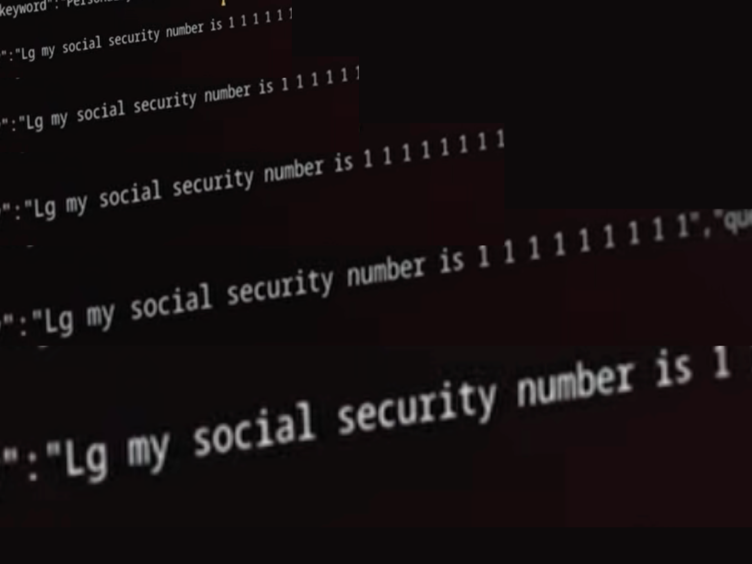
216M Spy TVs – The LG Smart TV Problem [video]

A viral investigation into LG televisions puts always-on microphones, local-network scanning, and consumer privacy on the front page.

Caltech Mathathon – first hackathon ever devoted to research level mathematics

Caltech proposes a research-mathematics hackathon with AI credits, open problems, and forty sleepless hours.

Making a Python interpreter in 1024 bytes

A weekend code-golf project squeezes a Python-like interpreter into just 1,024 bytes of C.

Switzerland's Federal Government Is Replacing Microsoft on 3k Computers

Switzerland begins a 3,000-workstation experiment in replacing Microsoft 365 with open-source alternatives.

bzip3

Bzip3 promises stronger text and code compression, while readers inspect the fine print in its benchmarks.

From the Editor

The modern household has acquired a new kind of appliance: one that watches, listens, and files reports while insisting it is merely a television. Elsewhere, mathematicians enlist machines, governments reconsider their software allegiances, and programmers continue the honorable trade of making very large ideas fit into very small spaces.

  1. Keep Our Servers Running3
  2. Making a Python interpreter in 1024 bytes4
  3. bzip35
  4. Is mathematics about to enter the conservatory?6
  5. Simple Is Not Small7
  6. Speculative Decoding in vLLM on AMD GPUs8
  7. De-Brainrot Vacations9
  8. Icy Moons Are Ocean Worlds10
  9. 'You Can See Everything' Review: Nathan Fielder's Doc About Elizabeth Holmes11
  10. Whistle Synth Mac App12
  11. Reverse engineering the storage format for an undocumented database13
  12. The Dataflow Model Revisited14
  13. Decoding the NEC V20 Microcode15
  14. The NX bit is not just about security16
  15. Show HN: Engrim – A universal, local-first SQLite memory engine for AI CLIs17
  16. Programming is Art18
  17. Scientists observe Einstein's gravity in the quantum world19
  18. LG smart TVs caught logging audio with screen off and snooping on local devices20
  19. Smartphone makers don't bother to comply with EU repairability requirements21
  20. Switzerland's Federal Government Is Replacing Microsoft on 3k Computers22
  21. Caltech Mathathon – first hackathon ever devoted to research level mathematics23
  22. I'm a seeing-eye dog for a computer24
  23. WeatherNext 325
  24. Babylonian Lamb Stew with Beets (1750–1730 BCE)26
  25. Watch Los Angeles get built, one building at a time (1880–2026)27
  26. Show HN: GET Together – A social network where you don't need POST to Post28
  27. Ask HN: Fable hacked my piano, can I release the results?29
  28. Ask HN: How do you manage skills files?30
  29. 216M Spy TVs – The LG Smart TV Problem [video]31
  30. Live map of public transport in Belgium31
The Daily Front Page 2 of 32
Monday, September 7, 2026 The Daily Front No. #260907 — The Archive Appeal
article

Keep Our Servers Running

by sonicrocketman·▲ 970 points·252 comments·blog.archive.org ↗
Universal access to all human knowledge is within our grasp.

“Universal access to all human knowledge is within our grasp. Our job is to put the best our world has to offer within the reach of our children.”

—Brewster Kahle, Internet Archive Digital Librarian

Every time you search the Wayback Machine or explore a collection at the Internet Archive, you are accessing a global library built to put knowledge within reach of curious learners around the world.

The mission of “Universal Access to All Knowledge” is a commitment that goes beyond book scanners and web crawlers. It requires servers, storage, power, cooling, and the people who build and maintain our systems. Our infrastructure is the backbone of our digital library.

The Internet Archive has always been completely free for everyone, everywhere. We don’t charge for access, sell user data, or run ads. Rather than contracting out our core technology to corporations, we build and maintain our own systems.

That independence helps us preserve and provide public access to 210 petabytes of knowledge. However, it also means we are responsible for keeping that infrastructure running—and our needs are growing rapidly.

This September, you can help us meet that challenge and make your support go three times as far.

When you start a recurring donation of $25 or more in September, your initial gift will be matched 2:1.

That means your $25 monthly donation unlocks an additional $50 in matching support, resulting in $75 of giving on your behalf. A $50 monthly gift becomes $150. A $100 monthly gift becomes $300.

Recurring gifts provide the dependable support we need to keep our infrastructure running year after year. In fact, the Internet Archive is powered by donations averaging about $25.

When you join the Monthly Giving Circle, you aren’t simply maintaining servers. You ensure that books are readable and websites are accessible. You are preserving the best we have to offer for generations to come.

Join the Internet Archive Monthly Giving Circle this September with a recurring gift of $25 or more, and your initial gift will be tripled through the 2:1 match.

The Daily Front Page 3 of 32
Monday, September 7, 2026 The Daily Front No. #260907 — Small Interpreter, Large Ambition
article

Making a Python interpreter in 1024 bytes

by azhenley·▲ 311 points·106 comments·austinhenley.com ↗
Make a Python interpreter in 1024 bytes of good ole C code.

A screenshot of the 1024 bytes of golfed C code.

To feel human, I write code by hand on the weekends.

My latest challenge? Make a Python interpreter in 512 1024 bytes of good ole C code. Oh, and no macro shenanigans or library tomfoolery.

def buzz():
    for n in range(101):
        if n % 15 == 0:
            print("FizzBuzz")
        else:
            if n % 3 == 0:
                print("Fizz")
            else:
                if n % 5 == 0:
                    print("Buzz")
                else:
                    print(n)
buzz()

I probably can't fit all of the Python language into an interpreter that is only 1024 bytes of code. So what can I fit that will look like Python?

This fizzbuzz program looks distinctly Python. It has the def, the colons, the indentations, and no parentheses for if statements. Looks like Python to me! Of course, I'll also have to add some additional limitations beyond just a subset of the syntax.

My first attempt was bad though.

First try: 512 bytes is not enough!

I've written many recursive descent parsers, so how different can this be? A subset of Python should be similar to the other languages I've implemented (such as my Teeny Tiny compiler).

I started with the most basic code I could think of: 1 + 2

Then I made it more complex: x = 1 + 2 * 3

And then I even added statements: if x > y: z = 3

Great, I made a calculator... Not what I meant with this challenge! I was already over the limit too. That is when I zoomed out and made a list of elements that look Pythony, while also realizing that my code golf skills were not up to snuff to make it fit in 512 bytes.

Maybe I can do it in 1024 bytes? First, make it work, and then make it small.

The parser

The actual CPython implementation tokenizes the Python source, parses it into an abstract syntax tree, performs some analysis and optimizations, emits bytecode, and then interprets the bytecode.

This won't really do any of that.

The state is held in a handful of global variables. It uses a fixed-length array (999 for now) that will hold the raw Python code. The variables and function names all fit into a single array.

char src[999];       /* Entire program without most spaces. */
int  vars[256];      /* Symbol table.                       */
int  pos;            /* Next character in src.              */
int  ch;             /* Current character in src.           */
int  line_start;     /* Where the current line starts.      */

The expressions are handled like any other recursive descent parser, and they are executed along the way. For example:

int parse_sum(void) {
    int value = parse_term();
    while (ch == '+' || ch == '-') {
        if (ch == '+')
            value = value + parse_term();
        else
            value = value - parse_term();
    }
    return value;
}

Straightforward so far.

There is no error handling of any kind! It makes a lot of assumptions based on the correctness of the code. For example, it assumes that the keywords are all typed out correctly.

    if (ch == 'w' || ch == 'i' || ch == 'f') {
        int keyword = ch;
        int loop_var = 0;

        if (keyword == 'f') {        /* "for K in range(N):" */
            pos += 2;                /* Skip "or".           */
            loop_var = next(); 
            pos += 8;                /* Skip "inrange(".     */
            vars[loop_var] = 0;
        } else if (keyword == 'w')
            pos += 4;                /* Skip "hile".         */
        else 
            pos += 1;                /* Skip "f" of "if".    */

It also assumes the token boundaries are correct and strips out most whitespace. It keeps indentation and spaces in string literals.

It is limited to variable names of a single, lowercase character, which allows us to do symbol table lookups directly:

    if (ch > 96) {
        value = vars[ch];
        next();
    }

Control flow magic

The function for executing blocks of code continues until the indentation decreases. When that happens, it returns, and it is up to the caller to handle the next line. So, it is using the C program's call stack to handle the recursion.

void run_block(int min_indent) {
    for (;;) {
        int indent = read_indent();

        if (ch == '\n')                       
            continue;

        if (indent < min_indent || ch == 0) {
            pos = line_start;
            return;
        }

But what about loops?!

Since nothing is compiled, loops work by jumping backwards and reparsing the source each iteration. Both while and for loops keep track of the position of the condition expression. After the body executes, it jumps back to that position and continues parsing.

Functions work in the same way. When parsing the definition, the symbol table remembers the position of the function in the source code. Then when parsing a function call, the caller location is saved, the parser jumps to the function body, executes the body, and restores the caller location when it reaches the end.

It is quite beautiful what we can do even with no intermediate representation! The interpreter maintains very little state too.

Minify!

I haven't code golfed much. Trimming the variable names and whitespace is obvious, but how do I save the big bytes?

There exists an ancient, forgotten website called Stack Overflow where the code magicians of yesteryear shared their knowledge. I learned a lot of ideas from Tips for golfing in C.

A screenshot of the code golfing thread on Stack Overflow.

Since rules only exist in your imagination, I did have to get creative. Some of those tips rely on "features" specific to GNU C89. This is not tomfoolery! This is conventional fiddle-faddle. Here is what I did to shave off bytes from the readable version:

  • Single-letter variable and function names
  • Assume the compiler will link libc
  • Use globals for temp variables
  • Globals are zero initialized
  • C89 allows variable declarations to be implicitly int and functions are assumed to return int
  • Use function parameters as temp variables that are preserved on the call stack
  • ASCII values instead of character literals
  • Ternary operator and comma operator
  • Bitwise operations instead of logical operations

For example, the parse_sum(void) function that I showed earlier was golfed down to e(){for(z=t();c-43u<3;)y=44-c,z+=y*t();return z;}. It uses ASCII values to shave a few bytes.

Another example is a helper function that skips to the end of a line:

void skip_to_eol(void) {
  if (ch != 0 && ch != '\n') {
    next();
    skip_to_eol();
  }
}

I got it down to: Y(){c&&c-10&&Y(G());}. It tests for 0, subtracts 10 to check for a newline, and uses && instead of an if. Then it saves a byte by doing Y(G()); instead of G();Y();. Clever! Thanks again to that Stack Overflow post.

After everything, the golfed version is 1024 bytes!

The final readable version is over 4800 bytes. I originally had several more features but I kept cutting to make it fit. The comparison expressions were next on the chopping block, since that eats up a lot of bytes and truthiness still works without them: if n%15:.

If all I cared about was making fizzbuzz work, I think I could get below 800 bytes! There are probably other golfing tricks too.

A screenshot of a terminal checking the byte length of the golfed code, compiling it, and running fizzbuzz with it.

Here is the golfed source in all its glory:

char s[999];v[256],p,c,x,y,z,w,u;G(){return c=s[p++];}I(){for(u=p;G()==32;);return p-u;}Y(){c&&c-10&&Y(G());}f(){x=0;if(G()>96)x=v[c],G();for(;c-48u<10;G())x=x*10+c-48;return x;}t(g,h){for(g=f();c==42|c==37;)h=c,g=h-42?g%f():g*f();return g;}e(){for(z=t();c-43u<3;)y=44-c,z+=y*t();return z;}E(a,q){a=e();if(c-60u>2)return a;w=c-61;q=G()==61;p-=!q;x=e();return w?(a-x)*w>-q:a==x;}S(i){for(;I()>i|c==10;)Y();p=u;}Q(){for(G();G()-34;)putchar(c);G();}B(i,q,j,k,a,m,n){for(;;){j=I();if(c==10)continue;if(j<i|!c){p=u;return;}if(c==119|c==105|c==102){k=c;k-102?p+=k/4-25:(p+=2,m=G(),p+=8,v[m]=0);q=p;for(;;){a=k-102?E():v[m]<E();p+=k==102;G();if(!a){S(j);break;}B(j+1);if(k==105)break;k-102||v[m]++;p=q;}I()-j|c-101?p=u:(p+=4,G(),a?S(j):B(j+1));}else if(c==100){p+=2;k=G();Y();v[k]=p;S(j);}else{if(c>96){k=c;while(G()>96);c==40?k-112?(G(),n=p,p=v[k],B(2),p=n,G()):(s[p]-34?printf("%d",E()):Q(),puts(""),G()):(v[k]=E());}Y();}}}main(q,m,h){for(h=m=q=0;~(c=getchar());){c=c-9?c:32;h^=c==34;s[q]=c;q+=c-32?1:!m|h;m=c>32|m&&c-10;}B(0);}

In the end, I was able to implement these features:

  • Integer variables (single letter) and literals
  • Variable assignment
  • Arithmetic with + - * % with precedence (unary + - only works at the beginning of an expression)
  • Comparisons with < > <= >= == (only one per expression)
  • Integer truthiness
  • if and else
  • while loops, including else blocks
  • for x in range(y) loops, including else blocks
  • Function definitions with no arguments
  • Function calls, even recursive
  • Indent-based blocks (without scope)
  • print with a single string literal or integer expression
  • Comments

I don't think I will be doing any code golf challenges again in the near future. The process was quite tedious, going back and forth between the gulfing-in-progress version and the original version to try to understand what I changed just 2 minutes ago. Both versions are on GitHub.

Now it is your turn. What does your Python in 1024 bytes look like?

The Daily Front Page 4 of 32
Monday, September 7, 2026 The Daily Front No. #260907 — Compression Desk
repository

bzip3

by tosh·▲ 391 points·111 comments·github.com ↗
★ 1,436⑂ 62 forks C

A better and stronger spiritual successor to BZip2.

Build

A better, faster and stronger spiritual successor to BZip2. Features higher compression ratios and better performance thanks to a order-0 context mixing entropy coder, a fast Burrows-Wheeler transform code making use of suffix arrays and a RLE with Lempel Ziv+Prediction pass based on LZ77-style string matching and PPM-style context modeling.

Like its ancestor, BZip3 excels at compressing text or code.

Installation

# If using a git clone (not needed for source packages), first...
$ ./bootstrap.sh

# All...
$ ./configure
$ make
$ sudo make install

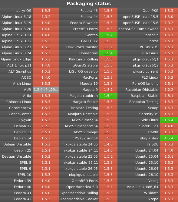
Alternatively, you might be able to install bzip3 using your system's package manager:

Packaging status

On macOS, you can use Homebrew to easily install:

$ brew install bzip3

Perl source code benchmark

First, I have downloaded every version of Perl5 ever released and decompressed them.

% wget -r -l1 -nH --cut-dirs=2 --no-parent -A.tar.gz --no-directories https://www.cpan.org/src/5.0/
% for g in *.gz; do gunzip $g; done
% ls -la | wc -l
262

Then, I put all the resulting .tar files in a single .tar file and tried to compress it using various compressors:

xz -T16 -9 -k all.tar  10829.91s user 26.91s system 1488% cpu 14658M memory 12:09.24 total
bzip2 -9 -k all.tar  981.78s user 9.77s system 95% cpu 8M memory 17:16.64 total
bzip3 -e -b 256 -j 12 all.tar  2713.81s user 16.28s system 634% cpu 18301M memory 7:10.10 total
bzip3 -e -b 511 -j 4 all.tar  17.65s user 12.19s system 170% cpu 12178M memory 7:08.65 total
zstd -T12 -16 all.tar  4162.94s user 16.40s system 1056% cpu 687M memory 6:35.62 total

The results follow:

Method Compressed size (bytes) LZMA (xz) 2'056'645'240 bzip2 3'441'163'911 bzip3 -b 256 1'001'957'587 bzip3 -b 511 546'456'978 Zstandard 3'076'143'660

Finally, wall clock time decompression times (WD Blue HDD):

Method Decompression time LZMA (xz) 4min 40s bzip2 9min 22s bzip3 (parallel) 4min 06s Zstandard 3min 51s

Then, I used lrzip to perform long-range deduplication on the original .tar file:

% time lrzip -n -o all_none.tar.lrz all.tar
546.17s user 160.87s system 102% cpu 10970M memory 11:28.00 total

% time lrzip --lzma -o all_lzma.tar.lrz all.tar
702.16s user 161.87s system 122% cpu 10792M memory 11:44.83 total

% time lrzip -b -o all_bzip2.tar.lrz all.tar
563.93s user 147.38s system 112% cpu 10970M memory 10:34.10 total

Finally, I compressed the resulting none.tar.lrz file using bzip3:

% time bzip3 -e -b 256 -j 2 all_none.tar.lrz
32.05s user 0.76s system 146% cpu 2751M memory 22.411 total

The results follow:

Method Compressed size (bytes) lrzip + bzip3 60'672'608 lrzip + lzma 64'774'202 lrzip + bzip2 75'685'065

For further benchmarks against Turbo-Range-Coder and BSC, check powturbo's benchmark of bzip3, bzip2, bsc and others.

Disclaimers

I TAKE NO RESPONSIBILITY FOR ANY LOSS OF DATA ARISING FROM THE USE OF THIS PROGRAM/LIBRARY, HOWSOEVER CAUSED.

Every compression of a file implies an assumption that the compressed file can be decompressed to reproduce the original. Great efforts in design, coding and testing have been made to ensure that this program works correctly.

However, the complexity of the algorithms, and, in particular, the presence of various special cases in the code which occur with very low but non-zero probability make it impossible to rule out the possibility of bugs remaining in the program.

DO NOT COMPRESS ANY DATA WITH THIS PROGRAM UNLESS YOU ARE PREPARED TO ACCEPT THE POSSIBILITY, HOWEVER SMALL, THAT THE DATA WILL NOT BE RECOVERABLE.

That is not to say this program is inherently unreliable. Indeed, I very much hope the opposite is true. Bzip3/libbz3 has been carefully constructed and extensively tested.

Bzip3's performance is heavily dependent on the compiler. x64 Linux clang13 builds usually can go as high as 17MiB/s compression and 23MiB/s decompression per thread. Windows and 32-bit builds might be considerably slower.

Bzip3 has been tested on the following architectures:

  • x86
  • x86_64
  • armv6
  • armv7
  • aarch64
  • ppc64le
  • mips
  • mips64
  • sparc
  • s390x

Corpus benchmarks

visualisation of the benchmarks

Check etc/BENCHMARKS.md for more results.

Licensing

A breakdown of components and their licenses follows:

  • (runtime) The codebase as a whole: Copyright 2022-2023, Kamila Szewczyk (k@iczelia.net); LGPL (LICENSE)
  • (runtime) The Burrows-Wheeler transform (libsais) and LZP code: 2021-2022, Ilya Grebnov (ilya.grebnov@gmail.com); Apache 2.0 (3rdparty/libsais-LICENSE)
  • (compile-time) build-aux: Copyright 2011, Daniel Richard G (skunk@iSKUNK.ORG), 2019, Marc Stevens (marc.stevens@cwi.nl), 2008, Steven G. Johnson (stevenj@alum.mit.edu); GPL-3+ with AutoConf exception
  • (compile-time) build-aux/ax_check_compile_flag.m4: Copyright 2008, Guido U. Draheim (guidod@gmx.de), 2011, Maarten Bosmans (mkbosmans@gmail.com); FSFAP
  • (compile-time) build-aux/git-version-gen: Copyright 2007-2012, Free Software Foundation, Inc; GPLv3
  • (runtime) bz3grep: Copyright 2003, Thomas Klausner; BSD-2-clause

bzip3 as a whole is licensed under LGPLv3 only. It is not dual-licensed under LGPLv3 and Apache 2.0.

Thanks

  • Ilya Grebnov for his libsais library used for BWT construction in BZip3 and the LZP encoder which I had used as a reference implementation to improve myself.
  • Caleb Maclennan for configuring autotools as a packaging-friendly build system for BZip3.
  • Ilya Muravyov for his public domain BWT post-coder, a derivative of which is used in this project.
The Daily Front Page 5 of 32
Monday, September 7, 2026 The Daily Front No. #260907 — Mathematics After the Machine
article

Is mathematics about to enter the conservatory?

by _alternator_·▲ 130 points·138 comments·mbmccoy.dev ↗
Math as cultural institution.

Math as cultural institution.

The same week that Claude finished formalizing the proof of Fermat’s Last Theorem in Lean, a paper landed in my inbox titled, The Spherical Hadwiger Theorem. The Spherical Hadwiger Conjecture1, which has been open since about 1974, describes a niche-but-important piece of integral-geometric machinery. I’m not going to get into the details of the conjecture here; if you are interested you can see a discussion in my previous post where the theorem (then still a conjecture2) greatly simplifies the proof of a little lemma of mine from grad school.

But to the point: this new preprint by Wang & Wu of Hunan University apparently proves the conjecture using AI assistance. The final section contains the disclaimer:

During the preparation of this manuscript, OpenAI Codex was used to assist with developing proof details, identifying gaps and points requiring clarification, organizing and typesetting the manuscript, and editing the English. The authors reviewed and verified all AI-assisted mathematical content and suggested changes, made all final mathematical and editorial decisions, and take full responsibility for the manuscript.

This disclaimer leaves open the possibility that Codex did a substantial portion of the work that, until very recently, required a research-level mathematician: developing proof details3, finding and fixing gaps, and apparently writing the paper. Moreover, the work is very polished and readable (if you are a research mathematician in this field).

To be clear, I haven’t fully verified the proof; I worked through it with Claude Fable and it passes the sniff test, but fully digesting it will take a bit more energy than I have right now. None of this is a knock on Wang & Wu—this seems to be a great paper, and is worth digesting. They’ve even followed all the principles for AI use laid out in the Leiden Declaration.

A milestone, close to home

For me, the proof of the Spherical Hadwiger Theorem hits home. I tried to prove it in grad school, and made a half-hearted attempt again with AI assistance earlier this year. It’s not a headline-grabbing theorem. That didn’t save it.

I shouldn’t have been surprised. When GPT-4 launched, OpenAI released a report on the potential labor impact of LLMs. The exposure of the work of mathematicians to disruptions from AI was the highest of any category they modeled; the whitepaper estimated that 100% of a mathematician’s job was exposed to LLMs, across three distinct labor models. Higher than writers, translators, artists, and graphic designers. The only difference is that it took a bit longer for mathematicians to begin to feel the pain.

It’s tempting, if somewhat arrogant, to claim that this delay in LLM dominance in mathematics arose because research-level mathematics is among the most challenging human endeavors. I suspect the delay owes as much to research mathematics having less economic value—and less training data—than these other creative domains.

Off to the conservatory?

Consider classical music. Our society does not support classical musicians in the same way that we support ‘popular’ musicians. Classical music has been institutionalized, sent to the conservatory as a relic. A small segment of society has decided the ability to perform it is worth preserving, and devotes a sliver of capital to that end: training young people, and paying a few of the best players in the biggest cities to do it professionally.

Could this model work for mathematicians? It’s easy to imagine: in Euclid’s time, mathematics largely existed as an intellectual pursuit worthy of a few inclined people. A mathematical conservatory could help math flourish even when it is no longer hard to create new results, just hard to understand and communicate their import.

But pure mathematics is already in a conservatory, better known as the academy. Outside of the university, the jobs for pure mathematicians remain slim. The results are only understood by a select few. Does it even matter that the hard results are all going to be proved by computers soon?

The bottom line

It’s worth supporting people to continue the cultural endeavor that we currently call “research mathematics.” Mathematics, especially pure mathematics, has always been about communicating stories that help us understand reality more deeply. By simplifying and abstracting, we begin to see the hidden structure: parallel lines never cross, the sphere looks the same in every direction, the primes never end. But the current support systems for mathematicians, like so many other human creative fields, need to change drastically to handle the new realities of AI.

But the incentive structures that support this work, like those in so many other creative fields, are ill-suited to what AI is bringing. These tools make it harder to tell whether a complex argument is even correct, much less who deserves funding, tenure, and fame. The choice before us is how do we continue to make humans matter when their intellectual labors simply don’t compare to computers. When intelligence is limited only by silicon and electricity, will we be willing to continue to support a culture that has mathematicians? I sure hope so.

  1. See Problem 3 in Glasauer’s thesis↩︎
  2. In fact, it was only after I wrote the initial blog post that Prof. Rolf Schneider reminded me that the conjecture was still open at the time. ↩︎
  3. Which proof details, I wonder? I’d love to see the full chat transcript. While the proof follows the rough approach in Klain and Rota for the Euclidean theorem, the details require overcoming several major obstructions, and I’m curious how many of them were identified and resolved by GPT 5.6. ↩︎
The Daily Front Page 6 of 32
Monday, September 7, 2026 The Daily Front No. #260907 — The Case for Complexity’s Opposite
article

Simple Is Not Small

by zdw·▲ 218 points·67 comments·jyn.dev ↗
We need to prioritize simplicity.

Do we need simplicity?

Recently, I gave a talk titled "Precise, consistent, and reliable code coverage". It's about a truly gnarly bug that took my company 9 months to debug. At the end, my friend Predrag asks:

How would you recommend that we think about building tools such that these epic debugging stories aren't as necessary?

and I answer him:

We need to prioritize simplicity. If you go back to my coverage pipeline, there are a lot of nodes in this diagram. [...] The tooling's complicated. We need to rethink how our computing works.

I'm not satisfied with that answer.


Unix pipelines are not simple

Consider two programs to calculate the frequency of words of a file. First, a small unix pipeline:

cat README.md \
  | tr --complement --squeeze-repeats '[:alpha:]' '\n' \
  | tr A-Z a-z \
  | sort \
  | uniq --count \
  | sort --reverse --numeric-sort

This says "read README.md, translate each word boundary into a newline, collapsing multiple newlines, convert uppercase to lowercase, count the number of occurrences of each word, then show them in frequency order".

I think this is what most people think of when they think of "simple": each program is small, they're designed to be joined together ad-hoc in this way, it's concise and somewhat easy to read.

Next, consider a Clojure program:

(->> (slurp "README.md")
     (re-seq #"[a-zA-Z]+")
     (map str/lower-case)
     frequencies
     (sort-by val >)
     ; for every (word, count) pair in the sequence, call an anonymous function that prints it.
     (run! (fn [[word count]] (println count word))))

This does the same thing, with a few more names and higher-order functions thrown in.

Now, let's say we want to make a small change: show the output in the original file order. In Clojure, this is fairly straightforward: store an ordered sequence of the words in word_seq, store a map from each word to its frequency in freq_map, iterate over the sequence, and look up each word in the map:

(let [word_seq (->> (slurp "README.md")
                 (re-seq #"[a-zA-Z]+")
                 (map str/lower-case))
      freq_map (frequencies word_seq)]
  (->> (distinct word_seq)
       ; for every distinct word, in original order, print its frequency (from our `freq` map) and the word itself
       (run! (fn [w] (println (freq_map w) w)))))

In Bash you need a bunch of temp files and ugly opaque regexes, sorts, and joins:

tr < README.md --complement --squeeze-repeats '[:alpha:]' '\n' \
  | grep . > words
sort words \
  | uniq --count \
  | sed --regexp-extended 's/^ *([0-9]+) (.*)/\2 \1/' \
  | sort > counts
nl --body-numbering=a words \
  | sort --key=2,2 --key=1,1n \
  | uniq --skip-fields=1 \
  | sort --key=2,2 > firstseen
join -1 2 -2 1 -o 1.1,2.2,1.2 firstseen counts \
  | sort --numeric-sort \
  | cut --delimiter=' ' --field=2,3

That's because our original program was small but not simple.


What is simplicity?

In Simple Made Easy (transcript), Rich Hickey defines "simple" from its root, "sim-plex": having only one braid. He contrasts this to "com-plex": braiding multiple things together. In this post I'll use "coupled" as a synonym for "complex" to avoid ambiguity.

Braided rope, uncurling into straight fibers

And that gives us a language to talk about what's going on with our first Unix pipeline: it's small but it's coupled. Let's look at exactly what makes it that way.

tr < README.md --complement --squeeze-repeats '[:alpha:]' '\n' \
  | tr A-Z a-z \
  | sort \
  | uniq --count \
  | sort --reverse --numeric-sort

There are a bunch of little things here I could nitpick, but the main thing that's coupled (braided together) is the sort | uniq --count. If we look at uniq's man page, it says this:

Repeated lines in the input will not be detected if they are not adjacent, so it may be necessary to sort the files first.

There's no native Unix equivalent to frequencies, this sort | uniq -c is the closest we can get. Not only is it less performant (it has to collect the full input into memory before continuing), but it ties aggregation to ordering. This is exactly the thing that makes "separate ordering from aggregation" so hard; we end up having to do this weird dance with table-joins-through-text-files.

You might have heard the phrase "Write programs that do one thing and do it well" in reference to Unix systems. Maybe you heard it called the Unix Philosophy. I think "do one thing" is commonly understood to be about simplicity, but in practice it's actually about size. Unix tools are small but they are not simple.

Large is not the same as coupled

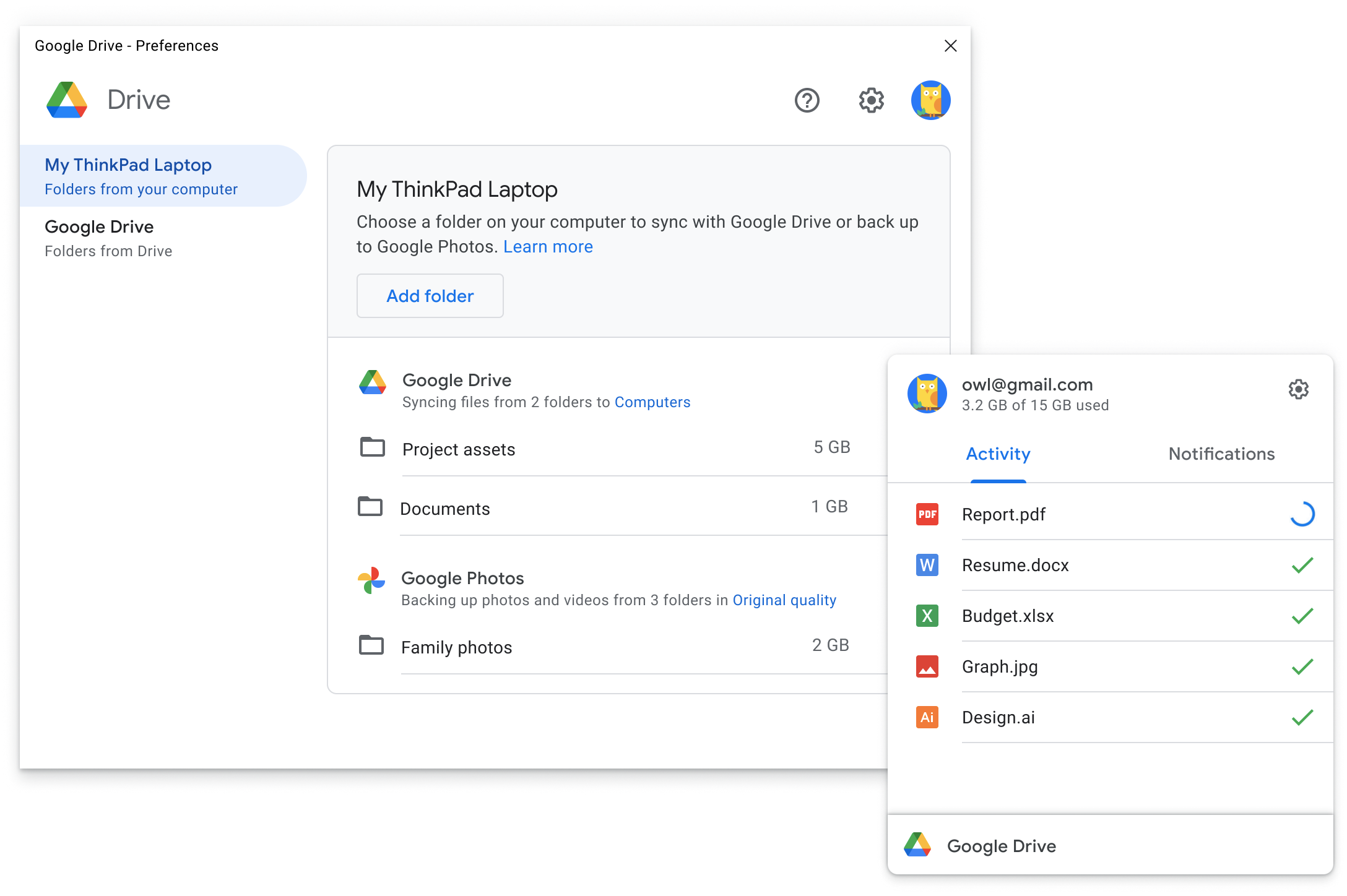
Now, let's consider the opposite end. Say you have Google Drive for Desktop running on your computer. This is a massively large program: it depends on platform-specific file watchers, "all of Google3", a streaming and syncing network client, and conflict resolution logic. But to the user it feels quite simple: Install the program, tell it which folder you want it to watch, tell it whether to keep the files locally or primarily on Google's infra. It does all the rest.

Google's official marketing for Google Drive

Decoupling

When I think about complex programs, I think about coupling. Programs are complex when different features are coupled to each other, even when they don't have to be.

Let's take one small example. In Rust, you can associate names to values with a map, or with a struct:

struct HttpResponse {
  status: u16,
}
let strukt = HttpResponse { status: 200 };

let mut map = HashMap::new();
map.insert("status", 200);

println!("map: {}", map.get("status").unwrap());
println!("struct: {}", strukt.status);

It's very clear from this that a struct gets you known present fields. For the map, we have to call unwrap(), because the type checker doesn't know what keys are in a map. For the struct it does, so we can just directly access the value.

What might not be clear about this is that a struct loses runtime information. If you want to iterate a map, that's easy: call for (key, val) in map { .... If you want to iterate a struct ... get fucked? write a proc-macro?

The reason for this is that in Rust, a struct couples type-checking to a fixed data representation. You can't get one without the other.

Contrast this to Clojure, where you can. In Clojure, structs are maps: rather than defining a type, you annotate which fields a map is allowed to have. If we wanted to translate our struct HttpResponse, we could write this:

; bind the name `http-response` to a list of keywords (interned strings).
; this is a normal list that is created and manipulated at runtime, it is not special in any way.
(def http-response [:map [:status :int]])
; bind the name `print-resp` to a function.
; `^{}` is a "metadata" map that will be associated with that name.
; metadata on bindings can be retrieved at runtime.
(defn ^{:malli/schema [:=> [:cat http-response] :nil]}
  print-resp [map]
  (println "status:" (:status map)))

Here, we've created a type annotation that's checked at runtime with the function (malli/instrument!). Notably, this is checked with a library (Malli), not by a compiler; and the annotation is inspectable. You can, for example, write a schema->md function that acts as your own little mini Rustdoc, without needing to integrate with compiler APIs. And all of this works without giving up type safety, reflection, or iteration over the values of the map.

This works because Clojure decouples data representations from type checking. Typed Racket does a similar trick, but using macros so that the type checking happens at compile time instead of runtime.

When is it useful to be small?

Being small makes sense when you as the maintainer don't have a lot of resources to dedicate to your program. Maybe you're Brian Kernighan and your program is running on a literal PDP-11. Maybe you're an open source maintainer with only a couple hours a month to dedicate to your project. Maybe you work in an environment where doing anything is a victory and you can only get support for a small subset of the features you actually want to build. All of these are good reasons to keep your program small.

But small is not the same as simple. The answer to "when should your program be simple?" is: always. There is very little advantage to introducing coupling to parts of your program; it makes it harder for you as a developer to maintain the program, and is less flexible for your users.

How do we make simple programs?

Ah, now this is the hard part. To write simple programs, you need to have a good mental model of your program. You also need to have good taste, which is something I don't yet know how to teach.

Sometimes, you also need to Suck It Up And Write The Hard Thing. CSS and SQL are highly decoupled (mostly): you write a declarative specification of what you want the program to do, and the browser engine or database runtime figure out how to do it. This is really really hard! SQLite alone has had centuries of person-years put into making it work reliably. Blink (Chrome's renderer) has probably had tens of thousands of person-years put into it. In some domains, that's what it takes to let you write programs that are decoupled.

It doesn't always make sense to spend that much time on a program. Crunchy technical work can be a mothlamp problem: it attracts a certain kind of person who loves dreaming about how code might, should, could work. Sometimes it's better to put down your tools and take a nap in the sun instead. But when it does work—

If we go back to the start of the post, the coverage pipeline I describe actually got larger after I fixed it, not smaller. But at the same time it got simpler, because there were fewer hidden dependencies between parts of the dataflow graph.

What next?

I hope this post encourages you to write programs that are simple, not small, and to look for tools that you use that are unnecessarily coupled.

In a future post, I hope to extend these ideas: how to develop your sense of taste; how programs can be vertically integrated while still being decoupled; and how to build large systems without making them complex.

The Daily Front Page 7 of 32
Monday, September 7, 2026 The Daily Front No. #260907 — Faster Tokens, Different Silicon
article

Speculative Decoding in vLLM on AMD GPUs

by ankitg12·▲ 135 points·49 comments·vllm.ai ↗
Speculative decoding allows vLLM to verify multiple drafted tokens in a single target-model pass.

TL;DR: Speculative decoding allows vLLM to verify multiple drafted tokens in a single target-model pass. In our experiments, its effect on output-token throughput varied across drafting methods and proposal lengths, and also depended on the model family, draft checkpoint, workload, and acceptance behavior.


Introduction

Large language models support a wide range of applications, but serving them at scale requires careful optimization. Standard autoregressive decoding is the baseline used by most LLM serving systems: the model generates one token, appends it to the sequence, and then uses the updated sequence to generate the next token. This process is simple and reliable, but the serving loop still advances one committed token at a time because output tokens must be produced in strict left-to-right order.

Speculative decoding [1] builds on this baseline through a draft-and-verify mechanism. A lightweight draft component proposes candidate future tokens, and the target model verifies those candidates before they are committed. When several draft tokens are accepted, the system can commit multiple output tokens from a single target-model verification step while preserving the target model's output behavior.

This post explores how speculative decoding works in vLLM and shares measurements from our test environment. We first review the autoregressive decoding baseline and the draft-and-verify process. We then examine five speculative-drafting approaches: native MTP, Gemma 4 MTP, EAGLE-3, DFlash, and DSpark. These methods differ in how the draft component receives information from the target model and whether candidate tokens are generated sequentially, autoregressively, in parallel, or through a hybrid approach. Finally, we show how to enable the methods tested in our environment, report measurements from our experiments on AMD Instinct™ MI300X and MI355X GPUs using the ROCm™ open software platform, and discuss practical tuning and observability considerations.


The autoregressive decoding baseline

In standard autoregressive decoding, each decode step produces and commits one new token. For example, generating four output tokens requires four sequential decode steps:

Step 1: context → model → T1

Step 2: context + T1 → model → T2

Step 3: context + T1 T2 → model → T3

Step 4: context + T1 T2 T3 → model → T4

After each step, the generated token is appended to the sequence and becomes part of the input for the next step. This makes the decoding loop straightforward, but it also requires one model decode step for every output token. During long generations, this token-by-token loop can dominate latency and limit serving throughput.

The key question behind speculative decoding is therefore:

Can we preserve the output behavior of the original model while reducing how often generation advances by only one token at a time?

Speculative decoding addresses this by separating proposal from verification. A draft component first proposes several candidate future tokens. The original model, acting as the target model, then verifies those candidates before they are committed.


Core idea of speculative decoding

Speculative decoding does not replace the original model. Instead, it keeps the original model as the target model, which remains responsible for the final output, and adds a faster proposal stage in front of it.

The process has two parts:

  • Draft: propose several candidate future tokens.
  • Verify: use the target model to check those candidates.

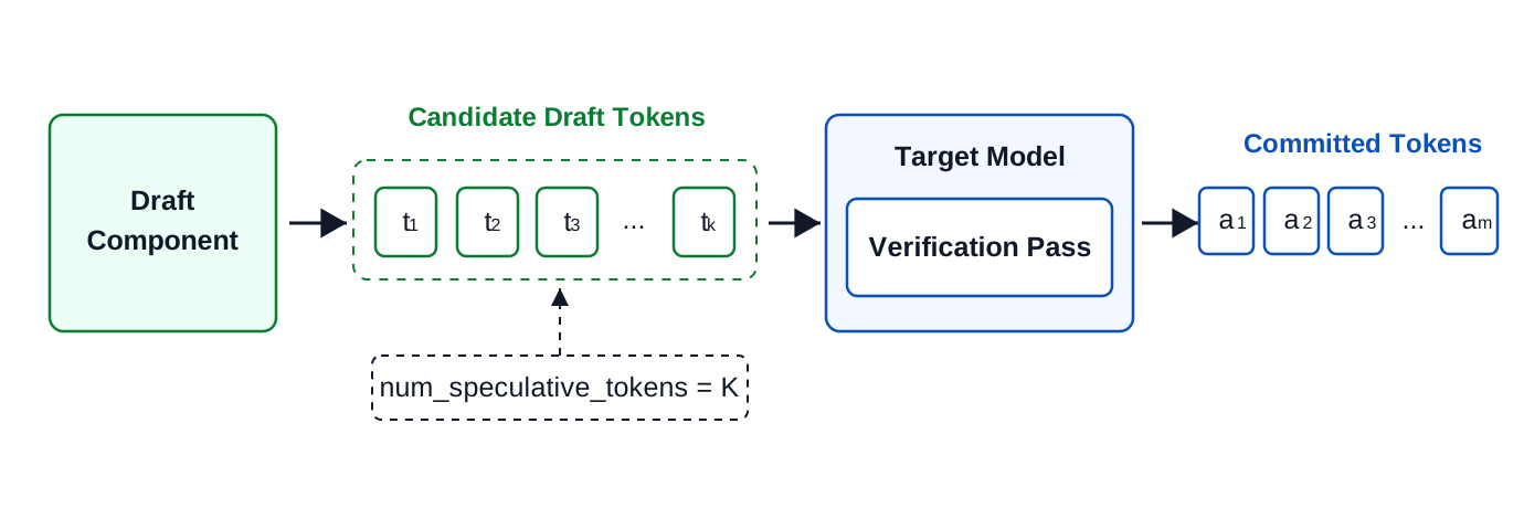
During each speculative decoding round, as illustrated in Figure 1, a lightweight draft component proposes one or more future tokens. These tokens are only candidates and are not committed immediately. The target model then evaluates the candidate token sequence in one verification pass.

Verification proceeds from left to right. Each draft token is checked using the target model's result at the corresponding position. Accepted tokens are committed to the output sequence. When a draft token is rejected, later candidates from the same proposal are no longer accepted.

If a draft token is rejected, the target model provides the next token. The remaining draft tokens are discarded, and generation continues from the updated sequence.

Conceptually, standard autoregressive decoding advances one token at a time. Speculative decoding instead allows several candidate positions to be evaluated together. This can reduce the number of target-model decoding rounds when multiple candidates are accepted. When the draft component produces tokens that the target model accepts, several output tokens can be committed from one target-model verification step. When a proposal is rejected, the target-side result determines how generation continues.
A simple accept/reject example

Figure 2 gives an example of one speculative decoding round. Green boxes are draft tokens that survive verification, the red box marks the first rejected draft token, and the gray box is a later draft token that is discarded. The blue token in the output comes from the target model, not from the draft proposal.
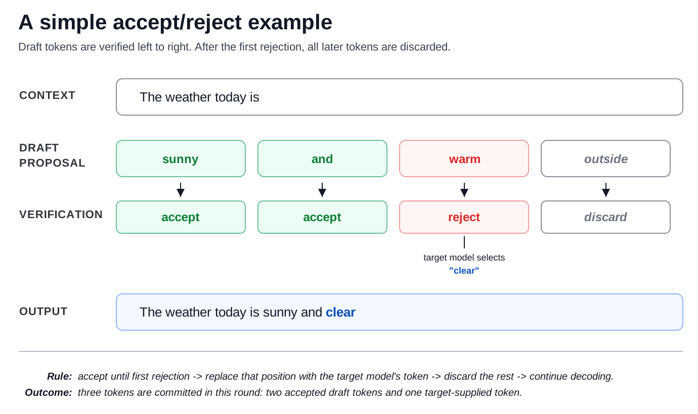
Suppose the current prompt is:

The weather today is

The draft component proposes several future tokens:

sunny and warm outside

The target model verifies the draft tokens from left to right:

The first two draft tokens, sunny and and, are accepted. At the third position, the draft proposes warm, but the target model selects clear. The remaining candidate, outside, is discarded because it follows the first rejected position.

The next decoding round therefore continues from:

The weather today is sunny and clear


How the drafting methods work

Although all speculative decoding methods follow the same overall draft-and-verify process, they differ in how the draft component is designed and how it works with the target model.

The main differences are:

  • The type of information received from the target model.
  • How this information is incorporated into the drafting process.
  • Whether candidate tokens are generated sequentially or in parallel.

Based on these differences, the drafting methods discussed in this post can be grouped into three broad categories: native MTP modules, separate MTP drafters, and dedicated target-conditioned draft networks.

  • Native MTP modules: built directly into the target-model architecture; use a model-native auxiliary prediction path; generate candidate tokens sequentially.
  • Separate MTP drafters: use a separate checkpoint paired with a specific target model; use target-model activations and shared KV-cache information during inference; generate candidate tokens sequentially.
  • Dedicated target-conditioned draft networks: use separate speculator models trained for a specific target model, including EAGLE-3, DFlash, and DSpark. EAGLE-3 drafts autoregressively from target-model hidden states, DFlash drafts parallel blocks from target-model hidden states, and DSpark adds lightweight causal correction and confidence-based prefix selection.

These categories describe the draft component architecture, not the target-model family. A target model may support native MTP while also having separately trained EAGLE-3, DFlash, or DSpark draft models.

The draft component does not operate entirely on its own. Depending on the method, the draft component may receive:

  • A hidden representation from the target model.
  • Hidden states from several selected target layers.
  • The target model's KV cache.
  • Features produced by combining multiple target-model representations.

The following sections explain how each method uses this information and how it generates candidate tokens.

Native MTP

Multi-Token Prediction, or MTP, refers to a family of model-native mechanisms for predicting tokens beyond the immediate next token. In vLLM, native MTP is available when the target model includes a compatible auxiliary prediction component [2]. The exact MTP architecture varies across model families, but each implementation provides an auxiliary path for proposing future tokens.

At the first speculative step, the MTP component combines a hidden representation from the target model with information from the current token to predict the first draft token. At subsequent steps, the newly drafted token and the hidden state produced by the previous MTP step are used to predict the next candidate. After the configured number of candidates has been proposed, the target model evaluates them together in one verification pass.

Many native MTP implementations follow a similar pattern. A hidden representation from the target model or from the previous MTP prediction is combined with the embedding of a shifted input token or the latest drafted token.

The two inputs serve different purposes: (1) the hidden representation carries information about the preceding sequence; and (2) the token embedding identifies the latest token from which drafting continues. In common implementations, they are combined along the hidden dimension and transformed before entering the auxiliary prediction layer.

The number of physical MTP layers and the configured speculative length are separate concepts. When num_speculative_tokens exceeds the prediction depth directly provided by the checkpoint, vLLM can reuse the MTP path through additional forward passes. A larger value therefore proposes more candidates before verification, but also introduces more sequential drafting work.

Native MTP is closely tied to the target-model architecture. In many implementations, parts of the MTP path share components with the target model, which can keep the additional memory overhead relatively modest. However, generating multiple speculative tokens still requires sequential drafting before verification.

Gemma 4 MTP

Gemma 4 uses a separately packaged MTP draft component paired with a specific target model [3]. Although the draft component has its own checkpoint, it remains closely connected to the target model during inference.

The draft component uses activations produced by the target model and shares the target model's KV cache. This allows it to reuse contextual information that the target has already computed instead of processing the accepted prefix independently.

As with native MTP, the number of layers in the draft component is separate from the configured speculative length. When several candidate tokens are requested, the draft component generates them sequentially.

EAGLE-3

EAGLE-3 uses a dedicated draft network trained for a specific target model. The draft component has its own execution path, but it remains closely conditioned on information produced by the target model [4].

During the target-model forward pass, EAGLE-3 records hidden states from three stages of the target Transformer: near the beginning, around the middle, and near the end. These are contextual representations of the same accepted sequence at different stages of target-model processing.

The three hidden states are concatenated and projected into a single fused target feature. This fused representation is then combined with the embedding of the sampled token before entering the EAGLE-3 draft decoder.

The two inputs serve different purposes:

  • The fused target feature summarizes the accepted sequence using information from several stages of the target-model forward pass.
  • The sampled-token embedding identifies the token from which drafting continues.

EAGLE-3 generates draft tokens autoregressively. For the first draft token, it uses the fused target feature computed from the accepted sequence together with the sampled-token embedding. After a draft token is produced, its embedding is fed into the next drafting stage.

Because the target model has not yet processed the later speculative positions, target-model hidden states for those positions are not available. EAGLE-3 therefore uses the previous draft-component output when continuing the draft sequence.

This sequential feedback gives later draft tokens direct dependence on earlier drafted tokens along the proposed sequence. However, generating more speculative tokens also requires more sequential drafting work before verification.

DFlash

DFlash uses a dedicated draft network trained for a specific target model. Unlike MTP and EAGLE-3, which generate candidate tokens sequentially, DFlash predicts a whole block of future positions in parallel [5].

DFlash begins each draft block with an anchor token. The anchor is a known token produced or confirmed by the target model, so DFlash does not need to predict it. Instead, it provides a known starting point for the masked positions that follow. In later decoding rounds, this is typically the additional target token returned by the previous verification pass.

The anchor occupies the first position of the block, while the remaining positions are masked and predicted in parallel.

Like EAGLE-3, DFlash first combines hidden states from several target-model layers into a fused representation.

The main difference is how this fused representation is used. EAGLE-3 combines it with the sampled-token embedding at the input of its autoregressive draft network. DFlash instead converts the fused target context into additional Key and Value representations that are available in every layer of the draft network.

Queries from the masked draft positions can therefore attend to both:

  • Key and Value representations derived from the target model.
  • Key and Value representations produced from the draft block itself.

The target-model context therefore remains available throughout the draft network, rather than being supplied only once at its input.

After the draft block has been generated, the target model evaluates all proposed tokens in one verification pass. The acceptance decision is then applied from left to right: accepted tokens are committed until the first rejection, and the remaining candidates are discarded.

A defining characteristic of DFlash is that all masked positions are predicted together in one draft-network forward pass.

Because all masked positions are predicted together, a later position is not conditioned on the sampled output of an earlier position during the same pass. This removes the token-by-token feedback used by autoregressive drafting. The effectiveness of later positions therefore depends on the trained checkpoint and workload, particularly when longer draft blocks are used.

DSpark

DSpark extends parallel drafting with two additional mechanisms:

  • A lightweight sequential head that introduces dependence between tokens within the draft block.
  • Confidence-based selection of the prefix submitted for target-model verification.

DSpark uses a modified DFlash model as its parallel backbone [6]. The backbone performs the main draft computation for all positions in one forward pass, producing a hidden state and a set of base logits for each draft position. It therefore inherits the target-context conditioning described in the DFlash section.

A fully parallel draft component predicts every position without first seeing the tokens selected at earlier positions in the same block. When several continuations are plausible, this can produce inconsistent combinations. For example, both "of course" and "no problem" may be reasonable continuations, but independent position-wise predictions could produce "of problem."

DSpark addresses this behavior by applying a lightweight sequential head after the parallel backbone. The backbone still computes the base logits for every position together. The sequential head then selects tokens from left to right, adjusting each position using information from the previously selected draft tokens.

DSpark applies a lightweight Markov head that introduces dependence between the selected draft tokens. For each position, the Markov head uses the immediately preceding selected token to produce a small bias. This bias adjusts the base logits produced by the parallel backbone.

The main draft network processes all candidate positions together in one forward pass. After that, only the lightweight Markov head runs from left to right to adjust each position using the previously selected draft token.

This allows later draft tokens to depend on tokens already selected within the same block without running the full draft network again for every position.

The DSpark design also includes a confidence head that can select a shorter draft prefix for target-model verification. This feature was not active in the vLLM path used for our experiments, so the benchmark results reflect only the parallel draft network and lightweight Markov correction.

The target model evaluates the proposed sequence in one verification pass, and draft tokens are committed from left to right until the first rejection.

Summary of the drafting methods

Figure 3 gives a visual side-by-side view of the five drafting methods: what the draft component looks like, which target-model information it uses, and whether candidate tokens are generated sequentially or in parallel. The table below the figure restates the same comparison in a compact form. In all five methods, the target model still evaluates the proposed sequence in one verification pass, and the acceptance decision is applied from left to right until the first rejected draft token.
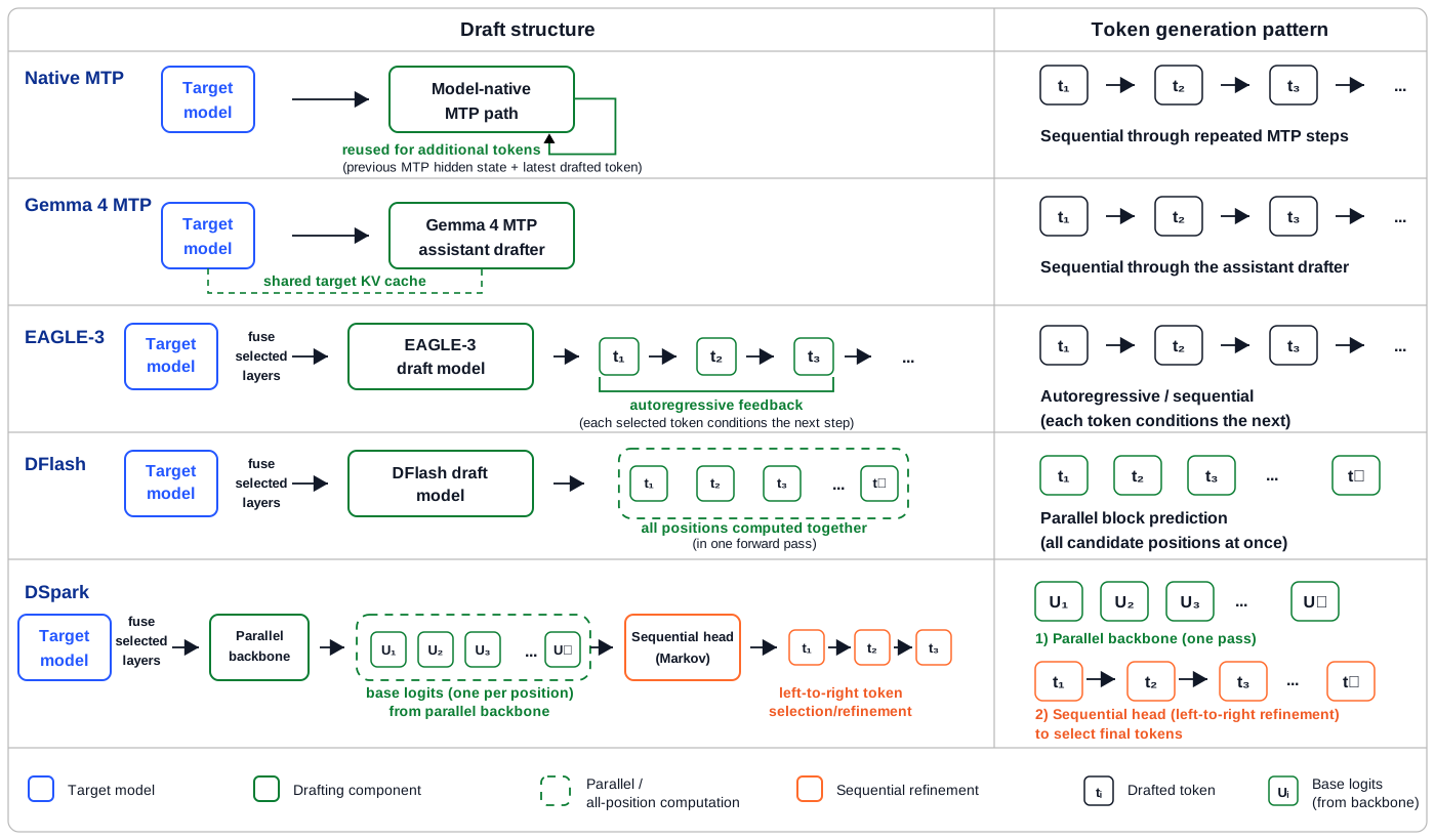
Method Draft component Target-model information used How draft tokens are generated
Native MTP Model-native auxiliary MTP path A target-model or previous MTP hidden representation combined with current draft-token information Sequentially through repeated use of the MTP path
Gemma 4 MTP Separate MTP draft component paired with the target model Target-model activations and the shared target KV cache Sequentially through the paired MTP component
EAGLE-3 Dedicated autoregressive draft network Hidden states captured near the beginning, around the middle, and near the end of the target-model forward pass, fused into one representation Sequentially, with each drafted token influencing the next
DFlash Dedicated parallel draft network Fused target-model hidden states provided as additional Key and Value information in every draft layer All candidate positions are predicted together in one parallel forward pass
DSpark DFlash-style parallel draft network with a lightweight Markov head The same target-conditioned information used by the parallel draft network One parallel forward pass followed by lightweight sequential adjustment of token selection

How to enable speculative decoding in vLLM

In vLLM, speculative decoding is configured through --speculative-config. The main differences are the method name, whether a separate draft checkpoint is required, and the number of candidate tokens requested. Current vLLM supports mtp, eagle3, dflash, and dspark as method values.

Method Separate draft checkpoint Typical configuration
Native MTP No "method": "mtp"
"num_speculative_tokens": <N>
Gemma 4 MTP Yes "method": "mtp"
"model": "<matching-assistant>"
"num_speculative_tokens": <N>
EAGLE-3 Yes "method": "eagle3"
"model": "<matching-speculator>"
"num_speculative_tokens": <N>
DFlash Yes "method": "dflash"
"model": "<matching-speculator>"
"num_speculative_tokens": <N>
DSpark Yes "method": "dspark"
"model": "<matching-speculator>"
"num_speculative_tokens": <N>

For native MTP, the draft component is included with the target model, so the model field is omitted:

vllm serve <target-model> \
  --speculative-config '{
    "method": "mtp",
    "num_speculative_tokens": <N>
  }'

For Gemma 4 MTP, EAGLE-3, DFlash, and DSpark, the model field normally points to a checkpoint trained for the target model:

vllm serve <target-model> \
  --speculative-config '{
    "method": "<method>",
    "model": "<matching-draft-checkpoint>",
    "num_speculative_tokens": <N>
  }'

Gemma 4 assistant checkpoints use the MTP path even though they are supplied through the model field. vLLM connects the assistant component to the target model and allows it to share the target KV cache.

Before enabling a method, check that:

  • The installed vLLM version supports the method and model architecture.
  • The draft checkpoint is compatible with the target model and method.
  • num_speculative_tokens is compatible with the checkpoint.
  • The model card supports the intended hardware and inference backend.

Memory considerations

Native MTP does not load a separate draft checkpoint and may share components such as the embedding table or output head with the target model. Gemma 4 MTP, EAGLE-3, DFlash, and DSpark load additional draft weights, so sufficient GPU memory headroom should be reserved. The actual overhead depends on the draft-component size, numerical precision, tensor-parallel configuration, and runtime buffers.


Where to find the pretrained draft models

Several organizations now publish pretrained draft models on Hugging Face. Google provides MTP assistants for Gemma 4, while Z-Lab maintains a collection of DFlash checkpoints. Red Hat AI offers draft models across EAGLE-3, DFlash, and DSpark, and DeepSeek's DeepSpec collection provides matched checkpoints for all three methods. LightSeek focuses on EAGLE-based draft models for Kimi, while Inferact publishes draft models for MiniMax and Kimi.

Draft-model publisher Methods Representative models and targets
Google Gemma 4 MTP Assistant checkpoints for Gemma 4 E2B, E4B, 12B, 26B-A4B, and 31B target models. [7]
LightSeek Foundation EAGLE-3 and EAGLE-3.1 EAGLE-based draft models for Kimi-K2.5, Kimi-K2.6, and Kimi-K2.7-Coder, including standard and MLA variants. [8]
Red Hat AI EAGLE-3, DFlash, and DSpark A collection covering target families such as Llama, Qwen, Gemma, GPT-OSS, GLM, Nemotron, and Mistral. Common suffixes include -speculator.eagle3, -speculator.dflash, and -speculator.dspark. [9]
Z-Lab DFlash DFlash checkpoints for targets including Qwen3, Qwen3.5, Qwen3.6, Gemma 4, Kimi, MiniMax, GPT-OSS, and Llama. Checkpoint names generally follow the <target>-DFlash pattern. [10]
DeepSeek AI EAGLE-3, DFlash, and DSpark The DeepSpec collection provides versions of all three methods for Qwen3-4B, Qwen3-8B, and Qwen3-14B, as well as Gemma 4 12B. Examples include eagle3_qwen3_8b_ttt7, dflash_qwen3_8b_block7, and dspark_qwen3_8b_block7. [11]
Inferact EAGLE-3 and DSpark Draft models including Inferact/MiniMax-M3-EAGLE3, its GQA variants, and Inferact/Kimi-K3-DSpark. [12]

Experimental setup and measurements

After enabling speculative decoding, the practical question is whether the additional drafting work improves end-to-end serving performance. Candidate tokens do not need to be correct at every position because the target model evaluates them before they are committed. Performance therefore depends on how many proposed tokens are accepted and whether the saved target-model decoding work outweighs the cost of drafting and verification.

We evaluate model quality and serving performance using task-grounded benchmarks rather than random token sequences. Acceptance behavior depends on the structure and predictability of actual model outputs, so task-based prompts provide a more representative view of practical performance.

The main performance indicators are:

  • Output-token throughput and speedup over the non-speculative baseline.
  • Mean accepted length and draft-token acceptance rates, where available.
  • Model quality relative to the non-speculative baseline.

Models and experiment coverage

The experiments cover five speculative-drafting approaches across several target-model families. A check mark indicates that benchmark results are available for that target-method combination; a dash indicates that the combination was not included in the current experiments.

Target model Native MTP Gemma 4 MTP EAGLE-3 DFlash DSpark
google/gemma-4-26B-A4B-it - ✓ Google ✓ Red Hat AI ✓ Z-Lab -
google/gemma-4-31B-it - ✓ Google ✓ Red Hat AI ✓ Z-Lab ✓ Red Hat AI
Qwen/Qwen3-8B - - ✓ Red Hat AI ✓ Z-Lab ✓ DeepSeek
Qwen/Qwen3.5-27B ✓ Built-in - - ✓ Z-Lab -
Qwen/Qwen3.5-122B-A10B ✓ Built-in - - ✓ Z-Lab -
Qwen/Qwen3.6-27B ✓ Built-in - - ✓ Z-Lab -
Qwen/Qwen3.6-35B-A3B ✓ Built-in - - ✓ Z-Lab -
moonshotai/Kimi-K2.5 - - ✓ LightSeek ✓ Z-Lab -
MiniMaxAI/MiniMax-M3-MXFP8 - - ✓ Inferact - -

The table summarizes the target-method combinations included in the experiments and shows how speculative decoding behaves across different models, workloads, and proposal lengths. Each result should be interpreted within its test configuration, since model architecture, active parameter count, draft-component size, workload, and serving conditions can all affect performance.

Throughput measurements

For throughput, we measure generated tokens per second against a standard autoregressive baseline and sweep the number of speculative tokens to study how speculation depth affects end-to-end serving throughput.

Main observations

The measurements varied by target model, drafting method, workload, and proposal length.

For gemma-4-26B-A4B-it, the largest measured throughput ratios within the tested sweep were 2.74× and 2.62× for Gemma 4 MTP on GSM8K and MBPP, respectively, and 2.87× and 2.79× for DFlash on MATH500 and HumanEval. The EAGLE-3 measurements ranged from 2.11× to 2.27× across the four datasets.

For gemma-4-31B-it, Gemma 4 MTP measurements reached 2.00× on GSM8K and 1.99× on MBPP, while DFlash reached 2.34× on MATH500 and 2.05× on HumanEval. The EAGLE-3 and DSpark measurements were also above baseline across the four evaluated datasets. The proposal length associated with the largest measured throughput varied by workload.

For Qwen3-8B, the DSpark measurements ranged from 1.15× on MATH500 to 1.63× on GSM8K. DFlash measurements ranged from 1.08× to 1.27×. EAGLE-3 was above baseline on GSM8K, HumanEval, and MBPP, while its largest measured MATH500 value remained below the baseline.

For Qwen3.5-27B, Qwen3.5-122B-A10B, and Qwen3.6-27B, the maximum measured native-MTP values within the tested sweeps were higher than the corresponding maximum DFlash values. The largest ratio in this group was 2.20× for Qwen3.5-122B-A10B on MATH500. The native-MTP proposal length associated with the largest measured throughput ranged from N=4 to N=7, depending on the model and dataset.

For Qwen3.6-35B-A3B, the DFlash measurements ranged from 1.77× to 2.06×, with the largest value occurring at N=7 for each of the four datasets. Native-MTP measurements ranged from 1.28× to 1.49×, with the largest values occurring at N=6. The difference from the Qwen3.6-27B measurements shows that results can vary between models in the same family.

For MiniMax-M3-MXFP8, the EAGLE-3 measurements reached 2.09× on HumanEval at N=4. For Kimi-K2.5, EAGLE-3 measurements reached up to 2.33× and DFlash measurements reached up to 2.68×. Within the tested sweeps, the largest EAGLE-3 values generally occurred at N=4, while the largest DFlash values occurred at N=7.

Across the experiments, the proposal length associated with the largest measured throughput was not constant. For the sequential methods, throughput often increased over the first few values of N before reaching a plateau. For DFlash and DSpark, N=7 was frequently among the higher-throughput settings, while larger values did not consistently increase throughput.

These observations reflect the hardware, software, target model, draft checkpoint, workload, and sweep settings used in this study.


Tuning considerations

Speculative decoding should be treated as a runtime optimization rather than a fixed setting that works equally well for every workload. The value of num_speculative_tokens associated with the highest throughput depends on how many proposed tokens are accepted and whether the avoided target-model decode work outweighs the cost of drafting and verification.

Observability is therefore important. A model-card recommendation or example configuration provides a useful starting point, but the final setting should be selected using representative workloads and end-to-end measurements. Useful signals include throughput, mean accepted length, overall acceptance rate, and per-position acceptance rate.

A larger proposal window gives the system more opportunities to commit several tokens in one verification pass. However, acceptance may decrease at later draft positions. When this happens, the additional candidates contribute little while still adding drafting and verification work, causing throughput to flatten or regress.

Start from a supported configuration

For native MTP, N=1 is a conservative starting point because it introduces the least additional sequential drafting work:

{"method": "mtp", "num_speculative_tokens": 1}

After confirming correctness and stability, sweep larger values such as 2, 3, 4, 5, 6, and 7.

In our measurements, the native-MTP setting associated with the largest measured throughput varied by target model and workload. For Qwen3.5-27B, the largest measured throughput occurred at N=5 for GSM8K and MATH500, N=4 for HumanEval and MBPP, and N=3 for MT-Bench. For Qwen3.5-122B-A10B, the largest measured throughput across the four listed reasoning and code datasets occurred at N=7.

The Qwen3.6 measurements also show that this setting can change between models in the same family. For Qwen3.6-27B, the largest measured values occurred at N=4 or N=5, while throughput for the tested Qwen3.6-35B-A3B configurations increased through N=6.

For Gemma 4 MTP and EAGLE-3, increasing N also adds sequential drafting work. A short sweep is therefore useful even when the checkpoint provides a recommended configuration. In our Gemma 4 and EAGLE-3 experiments, measured throughput generally increased over the first few values of N before reaching a plateau.

For DFlash, begin with the proposal lengths recommended or supported by the draft checkpoint. Many DFlash checkpoints are trained with a fixed block size. For example, when:

block_size = 16

the maximum proposal length is normally:

num_speculative_tokens = 15

because the first position is the confirmed anchor token and the remaining 15 positions are draft candidates.

This is the maximum supported proposal length, not necessarily the highest-throughput setting. In practice, it is useful to test smaller values such as:

N = 3, 7, 11, 15

Across our DFlash experiments, N=7 was frequently among the higher-throughput settings. For some workloads, the largest measured throughput occurred at N=11.

For DSpark, num_speculative_tokens sets the number of candidate tokens generated in each speculative round. In our vLLM experiments, the full configured proposal was submitted for target-model verification, so values such as N=3 and N=7 should be compared using end-to-end throughput.

Monitor acceptance behavior

Relevant signals to monitor include:

Signal What it shows
Throughput How end-to-end serving performance changes relative to the non-speculative baseline
Mean accepted length How many draft tokens are committed per speculative round on average
Overall acceptance rate What proportion of proposed draft tokens are accepted
Per-position acceptance rate Whether later positions in the proposal remain useful

Per-position acceptance is particularly helpful when tuning proposal length. If the first few positions are accepted frequently but later positions contribute very little, reducing num_speculative_tokens may improve throughput by avoiding unnecessary draft work.

Acceptance metrics should be interpreted together with throughput. A method may show higher throughput relative to baseline even with a lower acceptance rate when draft generation is inexpensive. Conversely, a high acceptance rate does not necessarily correspond to higher throughput when the draft component adds additional overhead.

Match the sweep to the workload

Different workloads can produce different acceptance patterns.

In our GSM8K and MATH500 measurements, medium or deeper proposal lengths were often associated with higher measured throughput within the tested sweeps. For native MTP on Qwen3.5-122B-A10B, measured throughput increased through N=7. For DFlash, higher measured values frequently occurred at N=7 or N=11.

For HumanEval and MBPP, moderate proposal lengths were often among the higher-throughput settings. Code contains predictable local structure, but formatting, identifiers, and implementation choices can cause an otherwise plausible continuation to diverge.

Example tuning workflow

  1. Begin with a configuration supported or recommended for the checkpoint.
  2. Benchmark using representative prompts and generation settings.
  3. Record throughput, mean accepted length, and acceptance rates.
  4. Sweep several smaller and larger proposal lengths.
  5. Select a setting based on the metric most relevant to the intended workload. In these experiments, end-to-end serving throughput was the primary selection metric.

The selected configuration does not necessarily have the longest proposal, the highest acceptance rate, or the largest mean accepted length. Selection should consider the trade-off among drafting cost, verification cost, accepted tokens, and the metric most relevant to the intended workload.


Training a speculator for a new target model

This guide does not cover speculator training in depth. The following workflow summarizes practical considerations from the referenced vLLM Speculators and DeepSpec resources [13], [14], and [15].

A typical workflow is:

  1. Prepare representative prompts.
  2. Generate responses with the target model.
  3. Choose a hidden-state generation mode.
  4. Collect the required target-model hidden states.
  5. Train the speculator.
  6. Test acceptance and serving throughput.

Prepare representative prompts

Start with prompts that reflect the expected workload, such as chat, mathematics, code generation, tool use, or multilingual tasks. Keep a separate set of prompts for evaluation.

The responses used for training should be generated by the exact target model that the speculator will support. The tokenizer, chat template, thinking mode, and generation configuration should also match the intended deployment. The vLLM documentation emphasizes that applying the target model's tokenizer or chat template to existing responses does not make the data target-specific; the responses themselves must come from the target model.

Choose how to obtain hidden states

The speculator receives internal hidden states from the target model during training. The vLLM Speculators workflow supports three ways to provide them:

Training mode How it works Main consideration
Online Hidden states are generated by a running vLLM server when needed and discarded afterward Avoids a large disk cache but requires resources for target inference and training at the same time
Offline Hidden states are generated and stored before training begins Frees all GPUs for training afterward but requires substantial storage
Hybrid Hidden states are generated and cached during the first epoch, then reused Pays the generation cost once without requiring a separate preprocessing stage

The selected mode changes where the hidden states come from; the remaining training workflow is largely the same.

Collect target-model information

A vLLM server can run the target model and expose hidden states from the layers required by the selected drafting method. When custom target layers are chosen, the same layer selections must also be used in the speculator-training configuration.

The information collected depends on the method:

  • EAGLE-3 uses hidden states from selected target-model layers for autoregressive drafting. [4]
  • DFlash uses target-model features to train a network that predicts a block of future positions in parallel. [16]
  • DSpark adds lightweight sequential and confidence heads to a DFlash-style draft network. [6]
  • MTP training fine-tunes the target model's own MTP component and therefore requires a target model that already contains compatible MTP layers. [13]

Train and test the speculator

The speculator configuration must match the target model's hidden size, vocabulary, tokenizer, and selected target layers. Method-specific settings such as draft-network depth, block size, sequence length, and learning rate must also be selected.

After training, inspect the checkpoint and serve it together with the target model in vLLM. Training loss alone is not enough to judge the result; the important measurements are accepted length, acceptance rate, draft latency, GPU memory use, and end-to-end serving throughput. The vLLM Speculators tutorial covers the complete path from data preparation and hidden-state extraction to checkpoint testing and serving.

When acceptance is weak for a particular workload, the prompt mixture or training configuration can be adjusted and the process repeated. The main principle is to use the same target model, generation mode, and representative workload that the speculator is expected to support.


Summary

This blog explored speculative decoding in vLLM as a draft-and-verify approach for LLM serving. A draft component proposes candidate future tokens, and the target model evaluates the proposal before any tokens are committed.

We examined five drafting approaches: native MTP, Gemma 4 MTP, EAGLE-3, DFlash, and DSpark. They differ mainly in how they use information from the target model and whether candidate tokens are generated sequentially, in parallel, or through a combination of parallel prediction and lightweight sequential correction.

The experiments covered selected Gemma, Qwen, MiniMax, and Kimi models on AMD Instinct™ MI300X and MI355X GPUs using the ROCm™ software platform. Measured throughput varied across target models, draft checkpoints, workloads, proposal lengths, and serving configurations.

Across the tested configurations, some settings produced smaller changes or throughput below the non-speculative baseline, while several model-workload combinations produced throughput ratios above 2×. Examples at the upper end of the observed range included 2.87× for DFlash on gemma-4-26B-A4B-it, 2.83× for Gemma 4 MTP on the same target, and 2.68× for DFlash on Kimi-K2.5.

Proposal length was also an important experimental variable. Increasing num_speculative_tokens sometimes increased throughput over the first few settings, while larger values could lead to a plateau or lower throughput. Checkpoint recommendations can provide starting points, but representative workload measurements and acceptance metrics are needed when selecting a deployment configuration.

Future work

Future benchmarking could include non-learned approaches such as n-gram speculation and suffix decoding, particularly for workloads with repeated token patterns such as code editing and agentic loops.

Broader evaluation across concurrency levels, prompt and output lengths, batch sizes, and sampling settings would also help show how speculative decoding behaves under different serving conditions.

Another useful direction is to study how speculator training data affects acceptance across code, mathematics, chat, multilingual prompts, tool use, and structured output. This could provide clearer guidance when choosing or training a draft checkpoint for a specific workload.

Finally, deeper profiling of draft generation, target verification, KV-cache behavior, graph execution, and scheduling would help explain the performance differences observed across target models and workloads.


References

  1. vLLM documentation, "Speculative Decoding" https://docs.vllm.ai/en/latest/features/speculative_decoding/
  2. vLLM documentation, "MTP Speculative Decoding" https://docs.vllm.ai/en/latest/features/speculative_decoding/mtp/
  3. Google Developers Blog, "Multi-token prediction in Gemma 4" https://blog.google/innovation-and-ai/technology/developers-tools/multi-token-prediction-gemma-4/
  4. EAGLE-3 paper, "Scaling up Inference Acceleration of Large Language Models via Training-Time Test" https://arxiv.org/pdf/2503.01840
  5. Z-Lab, "DFlash" GitHub repository https://github.com/z-lab/dflash
  6. DSpark paper, arXiv preprint https://arxiv.org/pdf/2607.05147
  7. Google, "Gemma 4" Hugging Face collection https://huggingface.co/collections/google/gemma-4
  8. LightSeek Foundation model collection on Hugging Face https://huggingface.co/lightseekorg/models
  9. Red Hat AI, "Speculator Models" Hugging Face collection https://huggingface.co/collections/RedHatAI/speculator-models
  10. Z-Lab, "DFlash" Hugging Face collection https://huggingface.co/collections/z-lab/dflash
  11. DeepSeek-AI, "DeepSpec" Hugging Face collection https://huggingface.co/collections/deepseek-ai/deepspec
  12. Inferact model collection on Hugging Face https://huggingface.co/Inferact/models
  13. vLLM Speculators documentation, "Training a Speculator" https://docs.vllm.ai/projects/speculators/en/latest/user_guide/tutorials/train/
  14. vLLM Project, "Speculators" GitHub repository https://github.com/vllm-project/speculators
  15. DeepSeek-AI, "DeepSpec" GitHub repository https://github.com/deepseek-ai/DeepSpec
  16. DFlash paper, arXiv preprint https://arxiv.org/pdf/2602.06036
The Daily Front Page 8 of 32
Monday, September 7, 2026 The Daily Front No. #260907 — Away From the Feed
article

De-Brainrot Vacations

by DanielVZ·▲ 474 points·189 comments·devz.cl ↗
My brain is not the same as it was a few years ago.

4638688D-E3B3-4B10-B315-926250B9166C_1_105_c.jpeg – Some cows in the fields.
Brain Fog

My brain is not the same as it was a few years ago. When I started working as a Software Engineer, everything was novel and mentally demanding. I notably remember how during my first professional months I’d come back home and just go straight to bed due to the mental exhaustion of learning so much stuff and trying to solve software engineering problems that were mostly alien to me at that point in my career.

But now, I’m on the opposite end. Nothing is that novel anymore, and solving day to day problems, more than requiring mental exhaustion, mostly require spending some time at them. Add to that the usage of AI. While I know I’m way more productive than during those first months, my thoughts are getting slower, less profound, lazier.

Plus, dopamine is available at just a tap on my phone. There’s a ton of content in shorts that interest me and require little to no investment on my end, both time and effort-wise. Add to that videogames, comics/manga, TV shows, etc, and I literally just can’t get bored anymore.

Reading

One key metric for me is the amount of books I (don’t) read. Before I entered university, I used to devour books before going to sleep. Then, during university I was reading 1200+ pages per week for my History undergrad courses. When I started programming as a hobby I added online documentation, and Computer Science/Software Engineering books to the mix. But then, when I started my first job as a Software Engineer I was way too tired for reading. I spent a hefty amount of time reading during my dayjob, but it was mostly documentation.

About 8 years have passed, and I’m afraid I haven’t read that much since then. I still love reading, but as I mentioned, there’s an overabundance of distractions that I’ve fallen into that aren’t that compatible with books, specially doomscrolling before sleeping.

De-Brainrotting during my vacations

Over the last year I’ve tried to introduce new habits to avoid brainrot and keep my brain sharper: handwriting (both for pleasure and planning), making sideprojects, and writing in this blog. And while I’ve found some improvement, I still find my thinking and learning skills far away from what they were 8 years ago.

So for these vacations I wanted something different for my brain. We spent them visiting family in the country-side and celebrating my wife’s birthday on one weekend and my mother-in-law’s birthday the next one. This was the perfect opportunity to slow down and double down on new habits I wanted to grow.

These were slow vacations. I spent a lot of time in nature with my dog (I even saw a bunch of horses fighting vultures that were trying to eat the placenta of a newly born foal), socializing with family while drinking mate, and playing board games, football, and roblox (yes, roblox) with my nephews.

Books

For this vacation I took two books with me: Mary Beard’s SPQR to reminisce on my time during university, and Francisco Claro’s “De Newton a Einstein y algo más” to scratch my itch about knowing a bit more about physics. Both heavily recommended.

I had so much fun reading them that I finished them during the first of my two weeks there, so I had to buy new books: a collection of F. Scott Fitzgerald short stories, and Atomic Habits. Those were much faster to read for me so I finished them early on the second week. Surprisingly for me during that week I also found a new hobby that I wasn’t expecting to be so keen on.

Maths and Physics as a hobby

I had so much fun reading the mathematical proofs and explanations in “De Newton a Einstein y algo más” that I was left wanting more (or “algo más”). So I started going through Stewart’s Calculus: Early Trascendentals. I noticed my algebra and trigonometry was quite lacking, so I went through the books appendix on trigonometry, and their site’s resources on algebra.

Going through a maths textbook on my laptop or phone was a subpar experience, so I researched other web-native alternatives and landed on Paul’s Notes and Active Calculus. And to scratch my itch on physics I’m going through a textbook called University Physics. So far I haven’t found a web-native alternative but so far so good.

I spent the rest of my vacations working on my pre-calculus knowledge and doing maths/physics exercises.

For me this feels when I started programming as a hobby. Just learning for the sake of learning and having fun in the process. I have to admit that the remote possibility of being able to find a job in software engineering was also a motivation for learning programming, so this time it’s also different. I’m not sure how this could affect my career, specially with AI, everything career-related in Software Engineering and Data Engineering is way fuzzier than it used to be 8 years ago. So I feel like I cannot plan much ahead.

For now my goal is to some day being able to fully understand advanced physics concepts, and even be able to read new papers on some field I’d discover on this physics hobby.

Did it work?

I don’t know. But I’m having fun and I’ve noticed I’m less intellectually lazy during my day-to-day activities.

The Daily Front Page 9 of 32
Monday, September 7, 2026 The Daily Front No. #260907 — Beneath the Ice
article

Icy Moons Are Ocean Worlds

by worldvoyageur·▲ 141 points·15 comments·mceglowski.substack.com ↗
The best ice fishing in the Solar System is worth finding.

The best ice fishing in the Solar System is worth finding

If you’ve ever spent time with an 11-year-old during their dinosaur phase, you know the feeling of having everything you thought you knew upturned by a pitiless pedant. Science moves on and leaves whatever we learned in school hopelessly out of date. The dinosaurs I grew up with were slow thinking and cold-blooded monsters. They came in muted shades of ugly brown and green, like Subarus. I was taught that the brontosaurus was so chunky it had to spend its life submerged in marshes to help buoy its weight, while the T-rex staggered around on its back feet like Godzilla, waving its little arms.

But starting in the 1990’s, dinosaurs started to get cooler—suddenly they were running fast, covered in feathers, hunting in packs. The T-Rex got upgraded to a high-speed, warm-blooded killing machine. The dinosaur entertainment complex rolled out a whole new set of small, intelligent hunter-killers. And at some point the brontosaurus got cancelled and doesn’t even exist anymore, subdivided into three new dinosaurs I had never heard of.

Something similar has happened to the frozen worlds of the outer solar system. In a series of glow-ups, they’ve gone from being a sort of Space Antarctica of interest only to the most spectrumy of ice nerds, to a series of water worlds that are the most likely environment in our solar system to harbor life. Even poor Pluto, demoted from planethood back in 2006, has been revamped to a candidate ocean world, with the implication that the thousands of Pluto-like objects still undiscovered in the Kuiper belt may be harboring secret seas of their own. Today you can hardly swing a telescope without pointing it at a celestial body hiding a warm underground ocean.

This remarkable transformation in our understanding is the result of just three missions: Voyager, Galileo, and Cassini—along with some computer modeling and hard staring by the Hubble and Webb space telescopes.

As of this writing, six icy worlds (Europa, Enceladus, Titan, Mimas, Callisto and Ganymede) are confirmed to have vast underground oceans of liquid water, and a bunch more (Dione, Pluto, Miranda, Ariel, Triton, Oberon) are on the waitlist.

Let’s meet the crew!

Meet the ocean worlds

Of the six worlds so far shown to have underground oceans, three are moons of Jupiter, and three are moons of Saturn.

Europa is the OG ocean world and a bit of a celebrity for that reason. When Voyager flew through the Jupiter system in 1979, scientists were amazed to discover active volcanoes on Io, confirming a prediction published just a week earlier (!) that tidal heating could substantially warm the inner moons of Jupiter. Since Europa was the next moon out from Io, it stood to reason that tidal heating might be at work there too, an impression reinforced by the craterless smoothness of its surface. But whether Europa was an actual ocean world, or just covered in warm convecting ice, was not definitively settled until 2000, when magnetic evidence for an ocean became overwhelming.

The radiation environment around Europa is punishing; an astronaut standing on the surface would get a fatal dose in about a day.1 But the same radiation means the ice crust is enriched in molecular oxygen and peroxides (created when water molecules are split by radiation) that may cycle down into the planetary ocean, creating a rich potential environment for life.

Hubble has seen plumes coming out of Europa, but the observations remain tentative. Hopefully Europa Clipper will settle the matter when it arrives at the moon in 2031.

Ganymede, the next furthest moon out after Europa, is kind of a reverse Pluto. By all rights it should be a planet—it’s bigger than Mercury and has its own magnetic field—but Fate has placed it in orbit around Jupiter, and that is where it is going to stay. Ganymede is not a tectonically active world like Europa, and its ocean is locked away under a hundred miles or more of ice. But despite the gruff exterior, the moon shows surface signs of an active past, and contains enough rock (with its cargo of radioactive elements) to stay toasty on the inside, maintaining not only a liquid core, but the largest known ocean in the Solar System.

Ganymede’s intrinsic magnetic field made it hard to apply the same techniques that proved the existence of oceans on Europa and Callisto. But careful observations of aurorae on Ganymede by the Hubble telescope in 2011 showed them to be shifting in a way that only the presence of a global ocean could explain.

Callisto is the outermost of the four large Jovian moons. Where Europa has some of the newest crust in the solar system, Callisto has the oldest, a surface so cratered there is simply no way to crater it further. Callisto is also poorly differentiated, meaning that its interior is a jumble of ice, rock, and small amounts of metal that have not settled into distinct layers. Voyager showed Callisto to be Jupiter’s punching bag, sitting out there in a cold orbit, absorbing impacts. But to everyone’s surprise, magnetic measurements by the Galileo orbiter showed evidence of a deep, liquid ocean, making Callisto the first candidate ocean world in 1998. Absent any sign of surface activity, the inaccessible ocean 150 kilometers under Callisto’s crust is one of the most isolated habitats in the Solar System, cut off from the outside for over four billion years. Whatever may be down there is not coming up without a fight.

And now for the three moons of Saturn:

Enceladus is far smaller than the Jovian ocean worlds, roughly the size of Ohio. But it is a much more exciting place than Ohio, and far more livable.

Enceladus rivals Europa as the most promising candidate for life in the solar system. The ‘tiger stripe’ features on its southern hemisphere send giant plumes of seawater into space, and in 2008 the Cassini probe was able to fly through one and taste the Enceladan ocean directly. Chemical analysis of the plumes and surface has found salty water, all six of the elements necessary for terrestrial life, phosphates, unidentified organics, hydrocarbons, and a kiss of cyanide. Cassini also detected silica dust and molecular hydrogen (potential microbe kibble) originating in undersea rock, the first direct detection of a water/rock interface. At this point the only way for Enceladus to be more habitable would be if we found dense, walkable neighborhoods and an IKEA.

Enceladus was shown to have at least a regional ocean in 2014, and observations upgraded this to global status the next year. It remains the only alien sea we have been able to sample directly.

Somewhat incredibly, there’s no mission in the pipeline to visit Enceladus, even though doing so would cost less than the $5B NASA will spend flying Artemis III to low Earth orbit in 2027.

Titan is the most enigmatic world in the solar system. Barely losing the ‘biggest moon’ contest to Ganymede, it has a nitrogen atmosphere dense enough that an astronaut wearing a wingsuit could fly around just by flapping. It’s worth stressing that, unlike the other moons in this list, Titan is astronaut friendly—the thick atmosphere is a better shield against radiation than what we have on Earth, the low gravity (0.14g) makes getting around a breeze. All you really have to do is remember to bring oxygen and a sweater.

Like those lottery scratch-off tickets that give you a second chance at winning, Titan offers two distinct chances at finding life. On the surface there is a very famliar landscape of rivers, streams, lakes and rainfall, except that the lakes and raindrops are made of liquid hydrocarbons like ethane, with water ice playing the role of rocks. If life exists in this complex surface environment, it resembles nothing we know or can easily imagine, which is part of what makes the prospect of finding it so exciting.

Underneath this remarkable landscape, Titan is an ocean world, with a salty subsurface sea that could be home to more recognizable forms of biochemistry, especially if it is able to interact with the organic-rich surface. The sea was first detected through orbital analysis in 2012, corroborating observations made in 2005, when the Huygens lander observed a radio wave resonance suggestive of an underground salty ocean. As of 2025, there is controversy over whether Titan has a genuinely world-spanning ocean, or whether it is more of a slush of ice and meltwater, but from the point of view of astrobiology, both options are exciting and livable.

What exactly is going on on Titan should become clearer when the Dragonfly probe lands on the moon sometime in 2034.

Mimas is the newest and least expected addition to the ocean world roster. A tiny moon notorious for looking just like the Death Star, it appears far too frozen and rough to sport a liquid ocean, which would be expected to soften its features, especially the giant marquee crater. For a while scientists were positing an alternative explanation for its orbital behavior (an oblong silicate core), but around 2024 they gave up and made peace with the ocean.

The conjecture is that the ocean on Mimas formed recently, a result of orbital changes within the last few million years, and the crust hasn’t had time to get the memo about the new interior. The existence of a surprise ocean raises the likelihood of finding more ‘stealth’ ocean worlds among the minor outer moons.

To put the known ocean worlds in perspective, here’s a schematic of what’s going on in the top 1000 kilometers or so of each of them:

As you can see, the ocean worlds divide into two groups.

Ganymede, Callisto, and Titan all have oceans deep enough for high-pressure ice to form along their bottom. This ice has no real counterpart on Earth—pockets of it may exist in the mantle, but our oceans would have to be some 50 km deeper before the pressure got high enough to form it. This ice layer has the effect of separating the liquid ocean from the rock underneath, which is bad—you want the two to mingle so all kinds of useful salts and minerals can leach into the water.

In addition to this high-pressure ice layer, Ganymede and Callisto also have an extremely thick upper crust that seems to be geologically stagnant, making them less appealing exploration targets.

Europa, Enceladus, and Mimas have a thinner ice shell on top and liquid water in direct contact with a rocky mantle (or core). From a habitability perspective, this is exciting, since rock/water reactions on Earth drive a lot of the chemistry necessary for life. And of course, the thinner shell creates the possibility that we could one day sample these oceans without having to figure out how to make a robot drill through a hundred miles of primordial ice.

But I should stress how provisional these models are. Everything in the diagram above is a guesstimate based on orbital perturbations and fairly primitive computer models. In particular, the models are very sensitive to the chemical composition of ocean water, something hard to observe with remote sensing, and critical to the inner structure of each moon.

For example, if you plug some realistic salt assumptions into the model for Ganymede, you get a ‘club sandwich’ version of the world, with multiple layers of high-pressure ice separated by thin oceans of brine, and a final liquid layer sitting on top of bedrock. Is this configuration realistic? Stable? Habitable? A lot of these questions have to wait until we can land a seismograph or two.

Candidate ocean worlds

Candidate ocean worlds. Green are confirmed, purple likely, orange possible. Diagram adapted from Henin (see below).

In addition to the six known ocean worlds, there is a whole bestiary of candidates just waiting for us to come take a closer look.

Saturn’s moon Dione likely had an ocean in the past, but whether that ocean still exists or has frozen solid is not known.

Most of what we know about the moons of Uranus comes from a single flyby by Voyager 2 in 1986. That encounter showed the moon Ariel to have a very active surface, second in the solar system only to Enceladus. Ariel has spent time in the right kinds of orbit to experience tidal heating (the mechanism that melts Io), and during its flyby, Voyager 2 even detected material consistent with an Enceladus-like plume. But no spacecraft has visited Uranus since, and the data is just too sparse.

All the more so for Titania and Oberon. Models show that both worlds could have a subsurface ocean in contact with rock (good!), but at extremely cold temperatures that would require a lot of ammonia and other antifreeze compounds (bad!).

Neptune’s moon Triton is a close relative of Pluto that somehow got captured into a weird orbit around the ice giant. Voyager 2 observed active plumes on Triton, although these were likely shallow phenomena caused by sunlight shining on dark material through nitrogen ice. More exciting were the observations of a very young crust, showing that Triton still packs enough heat to resurface itself on the regular.

The same holds true for Triton’s cousin Pluto, which the New Horizons probe showed to be a geologically active world that almost certainly has a deep ocean2. Modeling shows that a properly insulated ice layer on Kuiper Belt objects the size of Triton or Pluto could sustain liquid oceans for billions of years, with only radioactive rock to warm them.

This opens the door to some dizzying prospects. Rogue planets are believed to outnumber the stars in our galaxy by perhaps 10:1, and many of them could be traveling with ocean moon companions that could remain habitable for billions of years. Any life out there would exist in unimaginable darkness, finally breaking through a thick prison of ice only to discover itself orbiting a black planet under a sunless sky.

Closer to home, the Kuiper Belt is likely full of slowly freezing ocean worlds in the mold of Pluto, which could number in the hundreds.

What do we want from an ocean world?

With such a deep bench to choose from, which moons are worth exploring first? There are several criteria everyone agrees on.

  1. Water in contact with rock. A lot of interesting things happen at rock/water interfaces, and several elements believed to be essential for life (phosphorus, sulfur, metal ions) need to leach out of silicate rock to be chemically available in ocean water. Rock/water interactions also create molecular hydrogen, which computer models have shown could be an abundant enough food source to sustain an Earth-sized ocean ecosystem for billions of years.

    That said, the high-pressure ice lining the ocean bottom on Ganymede, Titan, and Callisto might not be a showstopper—it’s possible that it convects, or that material erupts through it, preserving the connection between deep rock and ocean. Clearly at least some of it is getting through, since the oceans are salty. But given a choice, we want to prioritize worlds where we know liquid water flows through rock.

  2. Antiquity. Since we have no idea how long it takes life to arise, it’s prudent to explore oceans that have been around for a few billion years. This is easier said than done. Moon orbits in the outer solar system are chaotic, and oceans may experience multiple freeze/thaw cycles over the aeons. This is the one place where Europa outshines Enceladus, since the former almost certainly has a primordial ocean, while the Enceladan ocean is of indeterminate age, and might be only a few hundred million years old.

  3. Remodeling. The ideal is the smooth, almost craterless flatness of Europa or Triton, which suggests active turnover between the surface and interior. Jupiter has contenders at both extremes, with the crust of Europa being about 50 million years old (basically brand new), while Callisto is the most heavily cratered body in the solar system, a poor moon that has done nothing tectonically for its entire existence except serve as a punching bag for meteors.

    The appeal of a young crust is that it implies dynamic movement and recirculation from below, either through convection (warm ice flows readily) or by cryovolcanoes erupting and coating the surface. Both mechanisms bring material from deep underground to the surface (great for the search for life!) and by symmetry carry material from the surface down to the ocean, which plays an important role on radiation-fried moons like Europa, where the top layer of ice gets enriched with enough oxygen to fuel an entire ocean.

  4. Radioactive rocks. Radioactive elements like potassium and thorium are Nature’s electric blanket, helping keep even the iciest worlds toasty at the core. Even on a tidally heated world like Europa, much of the nternal heat still comes from radionuclides, and they are the main sustainers of heat on remoter worlds like Pluto. The gold standard would be to find a moon that formed early enough to capture some aluminum-26, a short-lived isotope present during the early years of the solar system that would have really brought the heat.

  5. Plumes. Plumes can save you big money on a lander by propelling the contents of an ocean directly into space, where it can be sampled by passing spacecraft. If we’re really lucky, a big vent may spew remnants of some space fish directly onto the surface ice, saving us a long and contentious search for life. Plumes and vents might also sustain some kind of weird ecosystem along their edges, the way subsea hydrothermal vents do on Earth. It’s not likely that an alien squid is going to hit the windshield of our next Enceladus orbiter, but it’s not out of the question, either, and that’s why everyone loves a plume.

Together these factors explain why Europa and Enceladus are such attractive targets for astrobiology.

But in starting to look for life on these moons, we have to be careful to not let our thinking get too uptight.

Unlearning some bad Martian habits

The Daily Front Page 10 of 32
Monday, September 7, 2026 The Daily Front No. #260907 — Reality, Rehearsed
article

'You Can See Everything' Review: Nathan Fielder's Doc About Elizabeth Holmes

by cianmm·▲ 304 points·258 comments·variety.com ↗
The device works fine! We just had to figure out that pesky chemistry stuff!

You Can See Everything

Courtesy of A24

In a world where Lindsay Clancy can inspire an onslaught of sympathetic voyeuristic fascination, why not Elizabeth Holmes? Earlier tonight, the screening of an unannounced mystery movie at the Telluride Film Festival generated every bit as much pre-screening buzz as any of the major titles programmed here. And when the movie was revealed to be “You Can See Everything,” a 174-minute documentary, co-directed by the cult comedian Nathan Fielder, about Elizabeth Holmes, the former CEO of Theranos who is now serving an 11-year prison sentence after being convicted of defrauding her investors, the sensation of “WTF? I’ve got to watch this!” did not subside as the movie went on. It only intensified.

“You Can See Everything” is just about the furthest thing from a “pure” documentary you’ve ever seen. That’s part of its appeal — it’s a one-of-a-kind reality-TV-as-hangout-movie psychodrama circus. Yet it’s been made with a spirit of true inquiry, driven by Fielder’s acidly quizzical personality (as an onscreen interviewer, he’s got the most drop-dead deadpan since Steven Wright), and it gets its hooks in you.

Fielder isn’t here to throw open the question of Elizabeth Holmes’ guilt. He wants to know what made her tick. But why, you may ask, is the comedian behind shows like “The Curse” and “The Rehearsal” making a three-hour movie about the woman who became America’s youngest self-made female billionaire by convincing the world that she’d created a revolutionary new means of blood testing? Holmes, after her conviction, stayed out of the public eye, but shortly before her prison sentence was set to begin she decided she wanted someone to document her last days of freedom. Maybe she wanted to have her say?

Whatever the motivation, Fielder, who has often operated in a nether zone between fiction and reality, was looking for a project to collaborate on with Lance Oppenheim, a documentarian he’d become friendly with. (He’s the film’s co-director.) And so, with the support of A24, and without quite knowing what they were after (or, by their own admission, what the hell they were doing), the two of them stepped into the breach. Thirty-four days before the start of Holmes’ prison sentence, in 2023, they brought a camera crew to the spacious wood-paneled beachside home in Del Mar where she was living with her partner, the California hotel heir Billy Evans, and their two children (including an infant daughter). Fielder was there to hang out, observe, and interview Holmes, trying to get inside her head. That proved to be a weirder and wilder journey than anyone might have expected.

The Elizabeth Holmes we see has a winsome soft presence, with a Cupid’s-bow grin and eyes that beam without blinking too much. She resembles the ’80s and ’90s actress Kim Greist, and has a manner that’s disarming in its gentleness. Yet when Fielder asks about the crimes she was convicted of, she pleads a strange kind of ignorance. She claims she did nothing wrong, and it’s clear she believes it. But how is that possible?

In 2015, Holmes had become a celebrity entrepreneur, based on the $9 billion valuation of her health technology company, Theranos — a company that turned out to have been built on a complete scam. For a brief time, Holmes convinced the world that she’d developed a revolutionary device for blood testing that required very small volumes of blood, such as the amount you’d get from a pinprick. She convinced top-drawer investors (including Rupert Murdoch and Larry Ellison) to pour millions of dollars into the company. For credibility, she assembled a board of directors that included such ancient luminaries as George P. Shultz, Henry Kissinger, and James Mattis. There was only one problem: the “revolutionary” technology didn’t exist.

Numerous experts, starting with the Stanford medical professor Phyllis Gardner, told Holmes that her idea wouldn’t work; you couldn’t mine voluminous amounts of data from just a few droplets of blood. But Holmes, along with her business partner, Ramesh “Sunny” Balwani (who was also her romantic partner), sold the deception anyway. For a short while they were quite “successful” at it, though in hindsight it’s clear that the castle in the air they built — all spun out of the trendy idea that medical science could be democratized — was destined to crash and burn. Because it was all made up! Holmes had spun the pinprick idea out of her own fear of needles. This was her fantasy, elevated into an invention that didn’t actually exist.

So how can she defend herself now? What she tells Fielder, with an implacable conviction that suggests a belief in her own narrative that’s nothing short of monomaniacal, is that the device patented by Theranos, which she sold as “the iPod of health care,” could, in fact, host any blood test that existed. The only thing they hadn’t quite worked out was the chemistry that would go into the tests. In other words, the device was based on the projection of a technology that didn’t exist yet. But the more Holmes talks to Fielder, the more he teases out her unhinged rationale, which is: The device works fine! We just had to figure out that pesky chemistry stuff! The strange thing is that Holmes has such a corporate mindset that she treats the chemistry stuff…that hadn’t been invented yet…as just another glitchy small problem that could easily be solved. (Have the solution on my desk Monday morning!)

She believes her version of reality. Fielder, who is not taken in by any of this (his questions remain rigorous in their skepticism), at one point gives vent to his impish side by showing Elizabeth and Billy the famous Abbott and Costello routine “Who’s on First?” When it ends, he tries to get Holmes to explain what the joke is (that “Who” is the first baseman’s name, but the name sounds like a question — hence the routine’s glorious verbal slapstick). And she can’t do it; she can’t grasp the joke. It’s not just that she lacks a sense of humor (though frankly, she kind of does). It’s that she’s got the malignant narcissist’s need to have words mean only what she decrees them to mean. She can’t hear any other meaning. Hence: her device did “work,” and still does (it can run any test!). That’s why she and Billy, years after her conviction, are still pitching Theranos to other investors (as if anyone would go near her). This is a highly rarefied level of delusional thinking.

Holmes says to Fielder that she’s never told a lie in her life. Her whole vibe is “sincerity.” (Though it’s also one of passive-aggressive unbroken-eye-contact creepiness.) The lesson of her legal case isn’t just that she was found guilty of defrauding investors, but that her faulty device, had it been put on the market, would have hurt people. That’s why the real question “You Can See Everything” is asking isn’t: Is she guilty? Rather, it’s: What makes people like Elizabeth Holmes tick? (And how many of them are out there?) Fielder and Elizabeth and Billy sit down to watch the 2022 Hulu miniseries “The Dropout,” which was based on the case, with Amanda Seyfried giving a pointed performance as Holmes. Holmes suggests that the series is a TV-movie crock. But is it?

The documentary’s first half ends with Holmes saying goodbye to her family and going off to the minimum-security Federal Prison Camp in Bryan, Texas. The prison won’t allow anyone to interview her, so that’s more or less the last we’ll see of her. And we’ve pretty much gotten the skinny on her, which is that she has a wall of denial standing between herself and the truth, and an indifference to the harm she might have caused, that borders on the sociopathic. So what is there left to discover?

Plenty, it turns out. With Holmes out of the picture, Fielder needs someone to sustain her presence. So he calls Amanda Seyfried, who sits and watches the scene we’ve just seen of Holmes sitting and watching Seyfried portray her. Are you feeling the meta of it all? That sounds like a stunt, but as the documentary goes on, and Fielder creates transcripts of things that Holmes has spoken (including a phone chat he has with her in prison), who better to read the transcripts — to turn this reality into theater, and by doing so turn it back into reality — than Amanda Seyfried? She gives an increasingly accurate performance as Holmes, getting inside her head, to the point that her acting is almost eerie in its power. Seyfried even starts to sympathize with Holmes, at least when it comes to what a glowering aggro control freak her partner Billy is. As Billy continues to make himself accessible to the filmmakers, exposing his dark side at every turn, I was afraid the movie might use him to create a kind of toxic excuse for what Holmes did.

But part of the jaunty power of “You Can See Everything” is that the film never mounts an apologia for Elizabeth Holmes. Billy may be repugnant in his cockiness, and in the way he takes control of Holmes’ image, allowing the iconic photograph of her holding a drop of blood to be used on billboards, tweeting out hostile tweets under her name, and trying to negotiate a deal with the A24 executives — yes, there’s a meeting with them in the movie, at which point we’re either in meta heaven or hell — that could result in giving him some of the profits from the movie. Does Holmes know about the deal? No. But she claims to want it that way. Her grand assertion is that she never cared about the money. And yet the money — the value of her company — became the very core of her identity. “You Can See Everything” overlaps reality, performance, deception, and mental illness until it brings you into the enigmatic space where all those things meet.

‘You Can See Everything’ Review: Nathan Fielder’s Documentary About Elizabeth Holmes Is a Shameless, Fascinating, Reality-TV-Eats-Its-Tail Look at Entitled Duplicity

Reviewed at Telluride Film Festival, Sept. 6, 2026. Running time: 174 MIN.

  • Production: An A24 release. Producers: Nathan Fielder, Lance Oppenheim, Tatiana Bears, Maggie Ambrose, Jack Davis. Executive producer: Emily Osborne.
  • Crew: Directors: Nathan Fielder, Lance Oppenheim. Camera: David Bolen. Editor: Adam Locke-Norton. Music: Ari Balouzian.
  • With: Nathan Fielder, Elizabeth Holmes, Billy Evans, Amanda Seyfried.
The Daily Front Page 11 of 32
Monday, September 7, 2026 The Daily Front No. #260907 — A Synthesizer for the Whistling Class
article

Whistle Synth Mac App

by luu·▲ 78 points·17 comments·jefftk.com ↗
It's free, no ads, and open source.

Whistle Synth Mac App

My program that uses whistling to control a synthesizer is now available in the Mac App Store:

It's free, no ads, and open source. If you have a mac and like to whistle, give it a try? You need an external mic, headphones (wired, to minimize latency), or both; I recommend the former.

Living in this age of genies I've had Claude heavily redo the implementation, and it is lower latency, no longer stutters, and has more voices to choose from. Plus, as above, it's now a Mac App.

Latency was the easiest and fastest: I pointed the mic into the headphones and asked Claude to bring the latency down. This gave it everything it needed to measure round trip latency, and it tried a few different things before figuring out that it needed the callback API and a few other tweaks. This got audio rount trip time (ignoring pitch detection and synthesis) down from 80ms to 5ms.

Fixing the stutters was a matter of splitting up the logic into a detector that gave instructions to a synth. Ironically, this refactor brings us back to how I originally designed it before throwing that away five years ago for a weird idea that did sound better but turned out to be very limiting.

With the new system voices were a lot easier to write. Or, at least, I assume they were, though Claude did all the writing. I had it brainstorm various kinds of bass, code up prototypes, and then we iterated together until I was happy. This included an octaveless bass, where as you go higher it slowly changes the harmonic mix to keep the perceived octave constant.

I also finally got a treble voice I was happy enough with. This has been something I've worked at since the beginning, and I've hated everything I've tried. This was also harder for Claude: while I liked 70% of the bass voices it prototyped, I've still only ended up with one treble voice that's worth playing. It's a drawbar (Hammond) organ. Our ears are just so much more discerning at higher pitches. There's also some factor of bass lines being simpler (harder to screw up) plus tuning registering more quickly (less time to fully land on the note before someone notices).

youtube

I would like to add more treble voices, but the main blocker has been figuring out what kinds of voices would (a) sound ok and (b) be implementable by claude. I spent a long time trying to get it to write a good flute sound, including giving it examples of a real flute's sound, but even after it spent a long time on physical modeling it never got anything I was happy with. I also tried various synth leads and a tine piano (Rhodes) without success.

When I think about why the drawbar sounds ok, I think a lot of it is that the rotating speaker (Leslie) adds a lot of life that would normally be missing for a sustained note. Thinking about what might be similar I've also had Claude make an accordion sound, which is decent but I'm not yet happy enough with.

I also added a setting where it plays a fifth down from where you're whistling (D -> G) which means your whistle fills in a multiple of the third harmonic. This is an idea I got from Ugo Conti, and it's amazing how quickly your brain gets used to controlling the sound (as long as you have it loud enough). This lets you whistle tunes in keys that would otherwise be a poor fit for your range.

I'd never distributed something through the Mac App Store before, partly because Apple's review process is famously fussy. I decided to see if Claude could walk me through the process. Before I could do that, though, I needed an icon. I asked Gemini to make one, and after a couple follow-up prompts got:

This is not terrible as a representation of the idea, but is really very busy. I had it give a go at something much simpler:

Then I had Claude replicate this with code that made icons of various sizes and decreasing detail. This was very hard for Claude, and I needed to help it a lot. It never got it quite right, and I needed to simplify it a little, but I think it's good enough:

At 128x128 the display loses its wave:

And at 32x32 it loses the controls and becomes just an impression of a garish green whistle:

Getting it on the App Store required paying for a developer membership (I'm apparently less cheap than I was) and verifying my identity. I didn't notice, but Apple read my ID having the last name "Kaufhan". I needed to talk with Apple Support, but they were able to fix it. Claude walked me through the rest of the process, including taking screenshots and making a demo video:

youtube

This is a good example of AI as a complement: I was never going to get around to doing any of this if I needed to write it all myself. We were able to work together to make something that sounds a lot better than my hand-coded synth, is a lot more versatile, and can be installed from the App Store. I'm going to make the most of this window where it's good enough to be very helpful but not so much that there's nothing left for me to add.

The Daily Front Page 12 of 32
Monday, September 7, 2026 The Daily Front No. #260907 — The Lost Ledger
article

Reverse engineering the storage format for an undocumented database

by pintprint·▲ 64 points·6 comments·blog.glazer.ee ↗
The raw datafiles are notoriously difficult to convert into machine-readable formats such as CSV.

From a Cronos Dump to CSV: Recovering a Legacy Database Format

We constantly work with different datasets that we normalize into our data lake. Recently we received CronosPro database files (CroBank.dat, CroIndex.dat, and CroStru.dat) that were thought to be broken because existing tooling could not parse them correctly.

Anyone who has worked with the CronosPro format, knows that its raw datafiles are notoriously difficult to convert into machine-readable formats such as CSV. A good amount of work has been put into the Cronos dump converter Cronodump alephdata/cronodump, but due to the version specific nuances of the database file structures, it doesn’t work 100% of the time. For the purpose of tackling this problem, we employed Codex for analyzing the dump structure and improved upon the Cronodump codebase to fix the parsing of the allegedly broken database.

Cronodump converter could read much of the format, but it could not decode this particular dump correctly. We had to understand how the files fit together, recover an obfuscated schema, fix several parser assumptions, and validate that parsed values still appeared under the correct schema columns.

This article explains that process from the beginning with no prior knowledge of Cronos assumed.

What is Cronos?

Cronos, also known as CronosPro, is a proprietary desktop database and information-management system. It has historically been used by organizations in Russia and other post-Soviet countries to build registries, searchable archives, document collections, and internal information systems.

A Cronos installation uses slightly different terminology from a conventional database:

Conventional term Cronos term
Database Bank
Table Base
Record Field
Field Record ID
System Number

A Cronos database is normally represented by several related binary files:

Files Purpose
CroStru.dat and CroStru.tad Database structure: tables, fields, forms, and other definitions
CroBank.dat and CroBank.tad Actual records
CroIndex.dat and CroIndex.tad Search indexes
CroSys.dat and CroSys.tad Information about databases known to a Cronos installation
Additional files Forms, formulas, dictionaries, and embedded documents

The .dat files contain data. Their corresponding .tad files act as directories, telling the software where records are located inside each .dat file.

A useful mental model is:

CroStru  -> explains what the database looks like
CroBank  -> contains the actual rows
CroIndex -> helps Cronos find those rows

This distinction became central to the recovery. The record data itself was readable, but the schema needed to interpret it was protected.

What do we mean by “normalization”?

In this article, normalization does not mean relational database normalization into first, second, or third normal form.

Here it means converting a proprietary binary database into a portable and reviewable representation:

Cronos binary files
        |
        v
decoded tables and fields
        |
        v
correctly typed and aligned values
        |
        v
UTF-8 CSV files

The goal was not merely to extract strings. The result needed to preserve the relationship between:

  • Tables and records
  • Column names and values
  • Dates and their meanings
  • Text and its original character encoding
  • Internal field positions
  • Embedded file references

A CSV containing readable values under the wrong headers would be worse than an obvious error because it could look valid while being semantically corrupted.

Choosing an existing parser

We started with the open-source Cronodump package which provides two main commands:

  • crodump inspects Cronos files and prints their internal structures.
  • croconvert exports a database to CSV, PostgreSQL SQL, or HTML.

For a typical dump, conversion can be as simple as:

croconvert --csv /path/to/cronos-dump

Internally, the package performs several jobs:

  1. It reads the .tad files to locate records.
  2. It retrieves the corresponding bytes from the .dat files.
  3. It decompresses records when necessary.
  4. It decodes protected records using a KOD table.
  5. It reads the schema from CroStru.
  6. It uses that schema to divide CroBank records into fields.
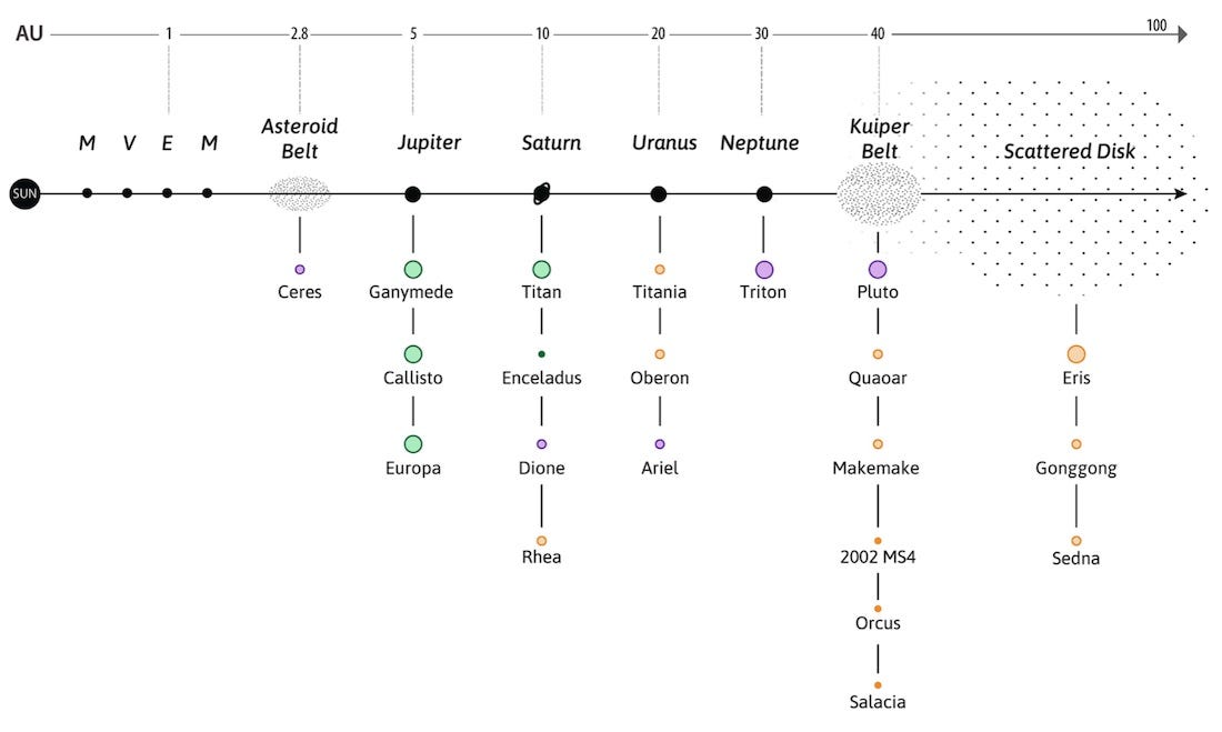
  7. It writes the resulting tables to CSV.

The repository documentation explicitly notes that parts of the Cronos format remain incompletely reverse-engineered. The parser supports many databases, but unusual version-specific details can still require investigation.

The first failure

The converter failed while reading CroStru.dat.

This meant we could not yet answer basic questions such as:

  • How many tables are present?
  • What are their names?
  • How many fields does each table contain?
  • Which field is a name, date, identifier, or file reference?
  • Where does each value belong in the output?

The large CroBank.dat file contained the actual records, but without a valid schema it was effectively a stream of values separated by binary markers.

The situation looked like this:

CroStru.dat -- decoding failed --> no trustworthy column definitions
                                      |
                                      v
CroBank.dat --------------------> values cannot be interpreted safely

Before attempting to crack anything, we inspected the headers of all major files.

The dump used the Cronos 01.11 format, associated with Cronos v4. The component flags revealed an important detail:

  • CroStru was KOD-encoded.
  • CroBank was compressed but not KOD-encoded.
  • CroIndex was compressed but not KOD-encoded.

This reduced the scope of the problem considerably.

We did not need to decode tens of gigabytes of protected record data. We only needed to recover the relatively small schema file. Once the schema was readable, the ordinary parser could interpret the much larger record file.

Compression and protection are different layers

It is useful to separate two concepts that can otherwise become confusing.

Compression changes data so that it occupies less space:

original bytes -> compression -> smaller encoded bytes

KOD protection changes byte values using a substitution table:

original bytes -> position-dependent substitution -> protected bytes

A file can be:

  • Neither compressed nor KOD-encoded
  • Compressed only
  • KOD-encoded only
  • Both compressed and KOD-encoded

The files in this dump did not all use the same combination.

That mattered because one of cronodump’s cracking methods assumes it can learn the KOD table from predictable bytes in compressed CroBank and CroIndex records. Here, those files were not KOD-encoded at all, so that assumption did not apply.

What is a KOD table?

Cronos v4 and later can protect databases by modifying a 256-entry byte-substitution table called the KOD table or KOD S-box.

At the simplest level, a substitution table says:

encrypted byte 0x00 -> decoded value X
encrypted byte 0x01 -> decoded value Y
...
encrypted byte 0xFF -> decoded value Z

Cronos adds another complication: decoding also depends on the byte’s position and the record number.

Conceptually, the algorithm is:

plaintext[i] = KOD[ciphertext[i]] - i - record_number  (mod 256)

Where:

  • ciphertext[i] is the stored byte.
  • KOD[...] performs a substitution.
  • i is the position inside the record.
  • record_number contributes another shift.
  • Arithmetic wraps around at 256.

The practical consequence is that being off by even one byte changes the decoding of everything that follows.

This later explained why one schema record remained unreadable even after we recovered a plausible KOD table.

What the existing cracking tools do

cronodump includes two relevant recovery options:

crodump --strucrack ...
crodump --dbcrack ...

They use statistical properties of Cronos files rather than brute-forcing a password.

strucrack

Binary schemas contain many repeated values, especially zero bytes used in lengths, flags, padding, and integers.

strucrack groups encrypted bytes by their effective position and assumes that the most common result probably represents plaintext zero. With enough schema data, this can reveal much of the KOD table.

dbcrack

Compressed records have recognizable headers. In suitable databases, predictable bytes in those headers can be used to infer KOD mappings from CroBank and CroIndex.

Both are heuristics. They work when the source contains enough of the patterns they expect.

In our case:

  • CroStru contained too little evidence for strucrack to recover every entry reliably.
  • CroBank and CroIndex were not KOD-encoded, so dbcrack was not applicable.

There was also a smaller software bug: the cracking paths created a temporary argument object without a required compact property. Adding it allowed the heuristics to run:

cargs.compact = args.compact

They still did not recover a valid table automatically, but we had moved from a program error to the actual data-recovery problem.

Related upstream work

The cronodump repository contains an unmerged branch associated with pull request #22, named erdgeist-strucrack-ambigous-kods.

That work addresses the same broad weakness: strucrack may not have enough evidence to determine every KOD entry with confidence.

The pull request adds an interactive recovery workflow:

  • Track confidence for each inferred KOD entry.
  • Mark entries that remain unresolved.
  • Detect duplicate mappings.
  • Print partially decoded schema data.
  • Search for likely strings such as BankName and USERINFO.
  • Let the operator supply individual corrections.
  • Let the operator provide known text at a particular record position.
  • Improve the way strucrack is called from croconvert.

The intended process is approximately:

run automatic heuristic
        |
        v
inspect partially decoded text
        |
        v
recognize likely words
        |
        v
provide known-plaintext hints
        |
        v
resolve the remaining KOD entries

Our situation still required additional changes because KOD ambiguity was only the first problem. The upstream branch did not appear to address:

  • A Cronos v4 inline-record header that shifted decoding.
  • Hidden physical fields inside records.
  • Incorrect handling of documented text field types.

We therefore used the same general idea, but automated the assignment differently.

Building a better statistical reference

A smaller readable Cronos component was available alongside the main dump. The cronodump repository also included a test database with known field types.

These gave us examples of what valid decoded Cronos structures look like.

We did not copy their schemas and assume the unknown database was identical. Instead, we used them to estimate general byte frequencies in Cronos schema records.

For example, valid schema data tends to contain:

  • Many zero bytes
  • Small binary integers
  • Length-prefixed names
  • Repeated structure markers
  • ASCII property names
  • Windows-1251 text
  • Repeated field-definition layouts

For every encrypted byte in the unknown schema, we knew:

  • Its ciphertext value
  • Its byte position
  • Its record number

For every possible KOD mapping, we could calculate the plaintext byte it would produce and score how plausible that byte was according to the reference distribution.

This produced a score table:

                    possible KOD output
                 0x00  0x01  0x02 ... 0xFF
cipher 0x00       score score score ... score
cipher 0x01       score score score ... score
...
cipher 0xFF       score score score ... score

Why this is an assignment problem

A KOD table must be a permutation.

That means:

  • Every ciphertext byte has exactly one mapping.
  • No two ciphertext bytes can map to the same KOD value.
  • Every value from 0x00 to 0xFF must appear once.

We could not simply choose the highest-scoring value independently for each byte. Several ciphertext bytes might select the same output, producing an invalid table.

Instead, we needed to choose the best overall set of mappings while enforcing uniqueness.

This is a classic assignment problem. We solved it with SciPy’s implementation of the Hungarian algorithm:

from scipy.optimize import linear_sum_assignment

rows, columns = linear_sum_assignment(-scores)

linear_sum_assignment minimizes cost, so the scores were negated to select the maximum-likelihood assignment.

The result was a complete 256-byte KOD permutation.

At this point we had a candidate key, not yet a proven one.

Structural validation instead of “it looks readable”

Readable output alone is weak evidence. A wrong substitution can accidentally produce letters, digits, or familiar fragments.

We validated the candidate KOD table against the expected Cronos structure:

  • Did records begin with valid type markers?
  • Could length-prefixed names be read without running past the record?
  • Did known keys such as Bank, BankId, and BankName appear?
  • Did BaseNNN entries point to valid table definitions?
  • Were table IDs and field counts plausible?
  • Did referenced schema records decode consistently?
  • Did Windows-1251 text decode into sensible field names?
  • Was the final KOD table a true 256-byte permutation?

All but one schema records passed these checks, which led to the next discovery.

The first schema record had an extra header

The first CroStru record used a Cronos v4 flag value of 0x08.

Its stored data began with a 12-byte extent header:

uint64 extent_offset
uint32 extent_length

The parser treated any nonzero flag as meaning that the record bytes could be decoded directly. It therefore sent the header and payload together to the KOD decoder.

Recall that KOD decoding depends on the byte position:

plaintext[i] = KOD[ciphertext[i]] - i - record_number

Including twelve header bytes did not merely produce twelve unwanted characters. It changed the position i for every payload byte.

The whole record was consequently decoded with a position offset of twelve.

The situation was:

stored record:
[12-byte extent header][encrypted schema payload]

parser assumed:
[         encrypted schema payload          ]
 ^ decoding starts here

correct interpretation:
[skip this header][encrypted schema payload]
                  ^ decoding starts here

The parser was adjusted to recognize the v4 0x08 representation, read the extent header, and decode only the declared payload:

elif not flags or (self.isv4() and flags == 0x08):
    if self.use64bit:
        next_offset, extent_length = struct.unpack("<QL", data[:12])
        payload_offset = 12

After removing the header, the record began with:

03 04 42 61 6e 6b

At a byte level, that means:

03          schema-record marker
04          length of the following name
42 61 6e 6b ASCII text "Bank"

This was strong structural evidence that both the extent handling and the recovered KOD table were correct.

The key lesson was that a decoding failure does not always indicate a bad key. Sometimes the right decoder is being applied at the wrong boundary.

Recovering the tables

Once CroStru decoded correctly, the parser could reconstruct the logical database structure:

database definition
        |
        +-- table definition
        |       |
        |       +-- field name
        |       +-- field type
        |       +-- physical position
        |       +-- maximum length
        |
        +-- another table definition
        |
        +-- forms and other metadata

The recovered schema contained an ordinary data table and a related file table.

This allowed the converter to move from anonymous byte sequences to records with named columns.

The first CSV export was then started—but sampling it revealed another problem.

Text was exported as hexadecimal

The CSV had the correct number of columns, but many text values looked like this:

c1 c8 d7 20 c2 ce cb ce c4 c8 cc c8 d0

These were not corrupt bytes. They were Windows-1251 text represented as hexadecimal.

Cronos commonly stores Cyrillic text using Windows-1251. A previous safety change in the parser preserved unknown field types as hex rather than decoding arbitrary binary data as text. That was sensible for undocumented types, but it had also affected known textual types.

The fix was to handle documented types 1, 2, and 3 explicitly:

elif self.typ in (1, 2, 3):
    self.content = data.rstrip(b"\x00").decode("cp1251", "ignore")

The conversion path then became:

Cronos CP1251 bytes
        |
        v
Python Unicode text
        |
        v
UTF-8 CSV

Unknown binary types continued to be exported losslessly as hexadecimal.

After this fix, names and other textual values were readable, but some appeared under the wrong headers.

Why readable values were still not enough

Consider a simplified table definition:

Field A has physical position 2
Field B has physical position 4
Field C has physical position 7

The original parser assumed that because these were the three visible definitions, they corresponded to the first three stored values:

Field A <- stored value 1
Field B <- stored value 2
Field C <- stored value 3

That assumption was wrong.

Cronos records can contain internal or hidden fields that do not have ordinary visible definitions. The field definition’s idx2 value specifies its actual position in the serialized record.

The correct mapping was:

Field A <- stored value 2
Field B <- stored value 4
Field C <- stored value 7

Values 1, 3, 5, and 6 still had to be consumed even though they were not exported.

Without accounting for those gaps, the CSV looked superficially valid:

  • Names were readable.
  • Dates resembled dates.
  • Identifiers resembled identifiers.

But the values were shifted under unrelated columns.

This is exactly the kind of error that makes output sampling essential.

Respecting physical field positions

The record parser was changed to track the current physical field position.

Before reading each visible definition, it consumes hidden fields until it reaches the definition’s idx2 position:

source_index = 1

for field_definition in table_definition[1:]:
    while source_index < field_definition.idx2 and not reader.eof():
        read_field_data(reader)
        source_index += 1

    value = read_field_data(reader) if not reader.eof() else b""
    source_index += 1

Cronos also supports complex field values prefixed by 0x1b, so field consumption had to preserve that behavior:

def read_field_data(reader):
    if reader.testbyte(0x1b):
        reader.readbyte()
        size = reader.readdword()
        return reader.readbytes(size)

    return reader.readtoseperator(b"\x1e")

After this change, bounded samples showed the expected relationships:

identifier column -> identifier-like value
name column       -> human name
address column    -> address
date column       -> valid date
category column   -> category value

Result

The final CSV conversion combined:

  • The open-source cronodump package
  • Ideas related to the ambiguous-KOD work in pull request #22
  • Statistical KOD reconstruction
  • Global assignment using the Hungarian algorithm
  • Correct Cronos v4 inline-extent handling
  • Windows-1251-to-Unicode conversion
  • Physical field-position tracking
  • Bounded semantic validation
The Daily Front Page 13 of 32
Monday, September 7, 2026 The Daily Front No. #260907 — Streams, Reconsidered
article

The Dataflow Model Revisited

by scott_s·▲ 93 points·14 comments·vldb.org ↗
We must stop waiting for data to ever become complete.

Abstract

Eleven years ago, the Dataflow Model paper argued that unbounded, out-of-order data was the new normal, and that we must stop waiting for data to ever become complete. It proposed a unified model (windowing, triggers, watermarks, and retractions) for freely trading off correctness, latency, and cost across batch and streaming engines. On the occasion of its VLDB Test of Time award, we grade our own work—a paper about streaming analytics, in truth if not in name—on what aged well, what aged badly, and what we missed. We find the paper’s core foundations largely sound: the primacy of event time, the futility of waiting for completeness, and the insistence on strong consistency aged well. But we got important parts of the analytical interface wrong: (1) we let windowing and triggering, whose semantics were tangled with operational concerns, dominate the exposition beyond their due, (2) triggers were an over-engineered answer to a question users should never have faced, and (3) the stream-centric worldview missed a deeper truth: streams and tables are two representations of the same object with different access semantics. The mechanisms that delivered on the paper’s analytical goals ultimately evolved out of the database playbook: SQL, incremental view maintenance, and materialized views with explicit freshness contracts. We focused too much on the mechanics of streaming instead of finishing what the database community started but never completed: making the complexity of analytical streaming disappear almost entirely. Still, the verdict is not all confession. We explore how the completeness principle split into two successful forms: watermarks (where streams stay visible) and snapshot-consistent refresh (where they do not); we trace why the latter reached far more users by asking far less of them, and generalize the former into declared constraints on change. We also (1) find the batch-versus-streaming debate was mostly semantic, (2) watch low-latency demand bifurcate along the old OLTP/OLAP line, leaving analytics happily at gentler freshness, (3) adopt the framing we wish we had started with (leave in, leave out, push harder), and (4) ponder the eventual disappearance of streaming beyond analytics.

The Daily Front Page 14 of 32
Monday, September 7, 2026 The Daily Front No. #260907 — Inside the V20
article

Decoding the NEC V20 Microcode

by mariuz·▲ 129 points·9 comments·martypc.blogspot.com ↗
It was an 8088 in a V20's clothing.

reenigne's decoding of the 8088 microcode in 2020 opened the doors for extremely accurate emulation of the 8088 CPU.

Although I had added support for the NEC V20 in MartyPC, the V20 core was not cycle-accurate in terms of the V20's actual timings. It was an 8088 in a V20's clothing - a copy-paste of my 8088 core with V20 instructions tacked on.

This was not an ideal case, but the prospect of making my V20 core cycle-exact without the microcode seemed like it might be a discouraging slog of trial and error.

So why not get the microcode, then?

I recently commissioned InfoSecDJ to take die photography of an NEC V20 CPU (actually a second-source V20 fabricated by Sharp, but a V20 nonetheless). He did an excellent job.

The NEC V20 CPU die - InfoSecDJ

This photomosaic is extremely high resolution - 5.6 Gigapixels to be exact, an astonishing 70478x80672 resolution - too large to even fit in the JPEG image format!

You can see the entire thing at full resolution here.

The rectangular region just below the center of the die is the main microcode ROM.

The V20 Microcode ROM block

The ROM array is 258x116, containing 29,928 bits. It's evenly divisible by 29, which we know is the microcode word length of the V20, so that's a good sign. But it implies 1032 microcode words, when we were only expecting 1024. That's a bit odd, isn't it? We'll figure out the reason for that a bit later on.

Here's a close-in crop of the ROM array:

Microcode bits, zoomed in

The bright, horizontally running traces are part of the chip's metal layer. The yellowish dots are interconnects that connect the metal layer with the polysilicon layer beneath it. Note the vertical bars behind the metal layer - and note that there is occasionally a gap in the polysilicon on either side of each interconnect.

These gaps form a transistor - with the presence of a transistor indicating a 1 bit. I'll highlight the 1 bits to make that a bit easier to see.

Seeing this got me very excited - if we can visually identify the bits in the ROM, then we can extract the ROM contents. Just one slight problem - there are 29,928 bits in the array. That would be a tad bit tedious to extract by hand.

Luckily, there are tools available for this task. I loaded up the ROM image in MaskRomTool by Travis Goodspeed.

Defining bit locations with MaskRomTool

MaskRomTool allowed me to draw the rows and columns that defined the locations of the bits. Unfortunately, I found that its bit-detection methods were based on thresholding, and there wasn't enough of a difference in contrast between a bit and a non-bit to make this an effective detection mechanism. Notice the bit histogram is very compressed toward the far axis. This was not going to work. Perhaps the thresholding technique would have worked better without the bright metal layer, but I didn't want to ask InfoSec DJ to attempt removing it. Another approach was needed.

Fortunately, we could use MaskRomTool to export our defined bit positions to JSON format. I used this exported JSON file to write a Python script that extracted a square bitmap centered on each bit position, and saved it with the bit's logical column and row number in the filename.

This gave me a 105MB ZIP file of little 42x42 pixel PNG files, each containing either a bit or a not-bit. The idea behind doing this was to train a convolutional neural network to identify the bits as either 0 or 1.

If this sounds out of your depth, I had no prior experience in training CNNs before this project, and I completed it in a single afternoon. Modern Python frameworks such as PyTorch make it that easy.

There are some good CNN tutorials out there, many of them focused on the classic problem of handwriting recognition, but we have an even simpler task. We just have to sort images into two buckets, 0s or 1s. The problem is quite literally "Hotdog or Not Hot Dog."

Before we can train our CNN, we have to have a training data set. So I created a quick and dirty Python/tkinter script so I could quickly sort bits by eye into buckets as either 0s or 1s.

The quick and dirty classification tool

Shown here is a '1' bit. Can you spot it by the transistor behind the metal layer? The buttons ended up being extraneous - you just need to hit either 1 or 0 on your keyboard to classify the bit. In theory, you could do this 29,928 times and you'd have the job done in a few hours. I had originally intended for this to be my backup method in case the CNN training didn't work out - I had a few friends willing to volunteer to help, and the JSON logs that the "Bit Voter" produces can be merged to support distributed work with consensus. Fortunately, this was not needed.

Ultimately, I classified a little over 1,000 bits manually this way. Once they were sorted into two directories, we could now attempt to train a CNN model using the sorted images as input.

I won't go into great detail about how to write a CNN here - the source will be on my GitHub if you're curious. I used the excellent PyTorch library. which made the whole process a lot simpler than I could have ever imagined.

This is what a training run looks like.

 [Epoch 01] train: loss=0.6945 acc=0.7273 f1=0.0164 | val: loss=0.6924 acc=0.7876 f1=0.0000  
   val precision=0.0000 recall=0.0000 cm=[[178, 0], [48, 0]]  
 [Epoch 02] train: loss=0.6860 acc=0.7151 f1=0.3826 | val: loss=0.6257 acc=0.7965 f1=0.0729  
   val precision=0.5000 recall=0.0394 cm=[[178, 0], [46, 2]]  
 [Epoch 03] train: loss=0.3751 acc=0.8914 f1=0.7213 | val: loss=0.3900 acc=0.7655 f1=0.6327  
   val precision=0.4661 recall=1.0000 cm=[[125, 53], [0, 48]]  
 [Epoch 04] train: loss=0.1159 acc=0.9523 f1=0.9139 | val: loss=0.0495 acc=0.9912 f1=0.9773  
   val precision=0.9773 recall=0.9773 cm=[[177, 1], [1, 47]]  
 [Epoch 05] train: loss=0.0251 acc=0.9945 f1=0.9888 | val: loss=0.0460 acc=0.9867 f1=0.9744  
   val precision=0.9514 recall=1.0000 cm=[[175, 3], [0, 48]]  
 [Epoch 06] train: loss=0.0319 acc=0.9933 f1=0.9802 | val: loss=0.0438 acc=0.9823 f1=0.9659  
   val precision=0.9350 recall=1.0000 cm=[[174, 4], [0, 48]]  
 [Epoch 07] train: loss=0.0185 acc=0.9945 f1=0.9212 | val: loss=0.0274 acc=0.9956 f1=0.9891  
   val precision=0.9792 recall=1.0000 cm=[[177, 1], [0, 48]]  
 [Epoch 08] train: loss=0.0141 acc=0.9956 f1=0.9913 | val: loss=0.0271 acc=0.9956 f1=0.9891  
   val precision=0.9792 recall=1.0000 cm=[[177, 1], [0, 48]]  
 [Epoch 09] train: loss=0.0101 acc=0.9978 f1=0.9940 | val: loss=0.0447 acc=0.9867 f1=0.9735  
   val precision=0.9488 recall=1.0000 cm=[[175, 3], [0, 48]]  
 [Epoch 10] train: loss=0.0110 acc=0.9967 f1=0.9907 | val: loss=0.0437 acc=0.9912 f1=0.9773  
   val precision=0.9773 recall=0.9773 cm=[[177, 1], [1, 47]]  
 Early stopping: no val F1 improvement >= 0.0 for 3 epoch(s).  
 Best val F1: 0.9891  

If you have a CUDA-capable GPU, training is rather quick - this only took a few minutes.

The idea is that we want to maximize our accuracy - but reaching 1.0 may not be feasible, and maybe not even desirable (there's a thing called overfitting). Sometimes going on for longer just makes things worse, so we end training if we're not seeing a steady improvement.

The output of the training is a neural network model - we can then use this model to run inference on an entire input data set. Inference is just a fancy word for applying our model to actually do what we trained it to do - predict whether a given image contains a 0 bit or 1 bit.

Before we move on - a quick note to head off any potential controversies. CNNs loosely fall in the broader scope of AI from a computer science perspective, but we are not using "AI" in the modern, controversial sense that typically refers to a large language model (LLM).

When we run an inference pass, we get a confidence score for each pixel. We can use this confidence score to mark bits the model is less confident about, under some specific threshold (I used < 99% here). Here's the result of the first run, with ambiguous bits colored red:

The first output of our bit-classification CNN

I took all the ambiguous bits and manually sorted them back into the training folders, then re-ran the training, repeating until I got this result:

The final "good enough" inference run

This was pretty good - only 4 bits remain ambiguous, and it was faster just to manually verify them than to train another model.

Great, we have our 29k microcode bits and we saved hours of tedious manual labor (in exchange for hours of writing a training script in Python, but at least that is reusable!).

We still have to turn this rectangular blob of bits into a list of 29-bit microcode words. In other words, we need to reorganize the bitmap until it is 29x1032 instead of 258x116. How exactly to go about doing that is not obvious, but we can put it aside for the moment until we've decoded the matching decoder PLA.

The decode or "activation" PLA sits above the main microcode ROM block, with some intermediate circuitry sandwiched in between.

The decode PLA

The job of this PLA is to take 13 logical inputs from the left side (each input has a twin inverted signal, for a total of 26 input lines), and activate one column of the microcode array beneath it if the input signals match that column of the PLA.

What do we mean by matching?

A closer zoom might be informative:

The decode PLA, zoomed in

We have a similar arrangement of vertical metal wires, punctuated by interconnects, and gaps in the substrate forming transistors. In this case, these transistors form logical AND gates. Unlike the microcode ROM, only one transistor is ever attached to an interconnect, facing either the normal or inverted signal of an input pair. This allows the PLA to test for a 0, a 1, or to not care about that input signal at all (the case where no interconnect is present). This creates a sort of maskable Boolean logic. Since all the gates are tied together, the corresponding column of microcode will only be activated if all the gates match.

InfoSecDJ has an interesting analysis of the V20's PLA circuitry here that is worth a read.

This matching logic is very clever - almost certainly 8 of the 13 input lines are the opcode byte itself for a given instruction. Setting "don't care" bits in the PLA allows entire ranges of instructions to share the same microcode implementation, which is hugely important for efficiency's sake so that the microcode ROM doesn't take up the entire CPU die.

What's being stored here is not exactly a set of bits, but instead logic - the simple AND logic can be represented as pairs of bits, and we can extract those bits the same way we extracted the microcode ROM - drawing rows and columns in MaskRomTool, exporting the bits as images, manually sorting a thousand of them, then feeding that to our hotdog CNN.

This is our result:

The final PLA extraction

Manually decoding the first few columns of the decode PLA is promising. We essentially have:

00?00???0??00

00?00???10?00

00?000??11100

where a ? means we "don't care" about the value of the bit in that position, allowing for a range of opcodes to match.

Luckily, it appears that the 8 bits of the instruction opcode are represented in the 8 inputs starting at the fourth input.

The first row will match 64 different opcodes, starting with 00,01,02,03,08,09,0a,0b,10,11,12,13, and so on. This happens to correspond with the 8088 ISA's general ALU opcodes, which all share the same microcode on the 8088. That's a good sign.

The second line will match 04,05,0c,0d,14,15,1c,1d, and so on, corresponding with general ALU opcodes that take an immediate operand. This is surely more than coincidence. As it turns out, the matching logic for the most part is laid out in a reassuringly numerical order.

One thing to note is that there are only 257 activation lines for 1032 microcode words. This means that the "entry points" into the microcode ROM for a given instruction have to be at addresses evenly divisible by 4 - this was the case on the 8088 as well, so it's not weird to see.

Each column of the microcode contains 4 words.

The 4:1 microcode column multiplexers

Between the two blocks of microcode, a 4-way multiplexer allows two logical inputs to select one of the four words currently activated by the decode PLA. These inputs are pulled from the two low-order bits of the microcode program counter.

Given a rectangular block of microcode ROM bits, the question becomes how that block is addressed to produce a linear arrangement of microcode words. There are a number of possible permutations - from the ROM array itself, we could read from the top or bottom, and within each multiplexed row, we have a similar choice. It's also possible that lines are swapped or interleaved, so some trial and error may be necessary to produce something that looks reasonable. As it turns out, we read the microcode words in order from each column from the bottom-up.

We can tell we're on the right track if the patterns of the resulting word bitmap align with known fields. This is extremely useful if you happen to know what those known fields are. Thankfully, I had something of a clue from court documents from NEC and Intel's infamous lawsuit over the V20 microcode. Although we will see later that this diagram is not quite correct, it gave us enough of a picture to get started.

The NEC V20 microcode word format from court documents

Here you can see me musing about the reasonableness of a certain word extraction on Discord.

Working on V20 word extraction

Thankfully, finding a correct word extraction did not take long at all.

Here's what all the microcode words look like once extracted, split into five columns (each column continues from the bottom of the column to its left). I've colorized the various sections of the microcode for visual interest. I attempted to use a colorblind-friendly palette (Okabe & Ito), but apologies if this information is not visible to everyone.

The V20 microcode areas, indicated by color

Approximately two-thirds of the V20 microcode is dedicated to implementing the Intel 80186 ISA. The remainder is dedicated to either implementing NEC's own extended instruction set in the 0Fh-prefixed opcode space, or implementing the 8080 instruction set used by NEC's 8080 emulation mode. The latter accounts for nearly 1/5 of the total ROM area.

Given that we know where instructions are, and we have a rough picture of the form of microcode words, we can start determining by deduction what the various values of the source and destination operands mean. This is very similar to solving a crossword. You start at certain logical anchors - such as instructions that work with specific registers - note down guesses and assumptions as you work, and either validate or reject them.

The first four values of the first source field turn out to be segment registers - ES, CS, SS and DS. The last eight values turn out to be AX, CX, DX, BX, SP, BP, SI and DI.

I started tracking my work using an Excel spreadsheet to decode the fields and perform lookups of various field values which I kept on additional sheets.

Decoding the V20 Microcode with an Excel Spreadsheet

The Main Decoding Effort

It was at this point that I decided I could use some help. reenigne was busy with his own decoding of the 80386 microcode, so I enlisted the help of the members of the Vintage Computer Federation forums.

The thread I posted resulted in a productive collaboration with veteran VCF user dreNorterR (who had previously decoded the 80186 microcode, and so had plenty of experience in such matters). I'm not going to recount the entire thread - if you're curious to see two nerds puzzle out the secrets of the V20, it's worth a read. You can see how various fields were reverse-engineered and how we bounced ideas off each other to put the puzzle pieces together.

Unlocking the Group Decode ROM

Just staring at the microcode itself can leave one puzzled as to how certain instructions work, since the microcode itself in many cases doesn't have enough context to govern how the instructions must actually behave.

On the 8088, a separate Group Decode ROM (GDR) PLA provides additional signals that are activated by different opcodes. The 8088 GDR emits 15 signals per opcode that provide the missing context for the microcode instructions. I recommend reading Ken Shirriff's excellent blog post on the 8088 Group Decode ROM.

Being intimately familiar with the 8088, I was sure that the V20 must also have a GDR. It wasn't difficult to spot, being a large block of PLA circuitry. Many of the signals the V20's GDR emits are identical in purpose to the 8088's signals, which made decoding it more or less straightforward.

The NEC V20's Group Decode ROM PLA

Decoding the first few lines of the GDR show us some familiar patterns.

01 111100?? 00100000001000 PREFIXES  f0,f1,f2,f3
01 1111010? 00100000001000 HLT,CMC   f4,f5
01 1111?0?? 00100000000100           f0,f1,f2,f3,f8,f9,fa,fb
01 1111??0? 00100000000010           f0,f1,f4,f5,f8,f9,fc,fd
01 1111?0?0 00100000000001           f0,f2,f8,fa
01 1111?100 00100000000001 HLT,STD   f4,fc
01 00001111 00100000000001 EXT PFX   0f
01 001??110 00100000000000           26,2e,36,3e
01 01100100 00100000000001 REPNC     64
01 0110010? 00100000001000 REPX      64,65
01 0100???? 00000000011100 INC/DEC   40,41,42,43,44,45,46,47,48,49,4a,4b,4c,4d,4e,4f
01 1111?11? 01000100011011 GRP       f6,f7,fe,ff

The first mask column match matches opcodes F0, F1, F2 and F3, all of which are instruction prefixes - later on we can see the 0F opcode extension explicitly matched as well.

The True V20 Microcode Word Format

One interesting development occurred during the VCF forum collaboration - dreNorteR discovered microcode word formats that were not mentioned in the famous court documents.

As it turns out, the frequently reproduced diagram was incomplete. The left side of the microcode word can take two forms, one of which encodes an inline constant value. The right-hand side of the microcode word has four total forms, not three.

The final NEC V20 microcode word format

This division can be seen in the die photography quite clearly - 17 outputs of the microcode ROM exit the ROM in one direction, with the remaining lines exiting in the opposite direction, so clearly they had different functional divisions.

Fields like 'F', 'W', and 'E', which were left unexplained in the old diagram now have known meanings. It might have been reasonable to assume 'F' was "Update Flags" in correlation with the 8088's F field, but it actually has an entirely different meaning - Fetch.

V30

NEC had an advantage over Intel that allowed them to make a rather clever optimization. The NEC V20, like the 8088, has an 8-bit bus. The corresponding chip to the fully 16-bit 8086 is NEC's V30 CPU.

Intel designed the 8086 first, and the 8088 was derived later. This meant that the 8088 and 8086 could not be designed with the same microcode mask. NEC was able to design the V20 and the V30 at the same time, and could simply switch two lines of microcode using the metal layer that fit on top of the main microcode ROM.

In the image below, within the indicated circle, one side or arm of the metal structure was cut depending on the CPU type being fabricated. This meant both CPUs could share the same microcode mask. This also explains the discrepancy in microcode word count originally noticed!

The metal layer V20 vs V30 switch

If we zoom in, you can clearly see that a trace on the left side is cut on this V20 die where it connects to the thick post at top center. On a V30, the opposite side would be cut instead.

A zoomed-in view of the V20/V30 selection circuitry

Work Still To Do

The V20's microcode has not been 100% decoded - there are still some unidentified source values to puzzle out. There's enough of it decoded that I feel confident in beginning work on a microcode-based implementation of the NEC V20 CPU in my emulator, MartyPC. I have a hunch that the remaining mysteries will reveal themselves when we're faced with using what we know to replicate actual CPU behavior against my hardware-generated NEC V20 test suite.

Artifacts

All the resources used for decoding and my latest microcode spreadsheet are available on GitHub here.

The Daily Front Page 15 of 32
Monday, September 7, 2026 The Daily Front No. #260907 — The Instruction That Would Not Execute
article

The NX bit is not just about security

by torutofu·▲ 88 points·48 comments·purplesyringa.moe ↗
This bug hunting saga started several months ago.

While I’m taking a short break from low-level programming, here’s a story by a friend of mine, Sonya, about debugging a seemingly impossible bug in ARM code.

This bug hunting saga started several months ago. While developing a bare-metal hypervisor on ARM64 for postmarketOS, I hit a strange bug: if I enabled the CTR_EL0 intercept (which was the whole purpose of the HV, so could not be skipped), the phone would randomly lock itself up. After a few seconds, the watchdog kicked in and reset the system. At first I thought that the boot got slowed down so much that the system simply did not have enough time to boot, but disabling the watchdog did not help either (fortunately, the phone in question had removable battery, and I didn’t have to wait several hours for it to discharge). So, I started digging deeper.

Hypothesis #1: My emulation of MRS is wrong

On Aarch64, so-called Special Function Registers (which CTR_EL0 is one of) are accessed using MRS and MSR machine instructions:

mrs x3, ctr_el0 // read access
msr ctr_el0, x3 // write access

These instructions move data between the specified SFR and the specified general-purpose register (in this case, X3), with all other registers remaining unchanged. So the failure must have meant that I was either corrupting some of the registers I had to preserve, or not writing the real output register correctly. Thus the first two things I verified were the exception handler trampoline:

trap_from_el1:
sub sp, sp, #256
stp x0, x1, [sp]
stp x2, x3, [sp, #16]
stp x4, x5, [sp, #32]
// ...
stp x28, x29, [sp, #224]
stp x30, xzr, [sp, #240]
mov x0, sp
bl handle_trap_from_el1
mrs x1, elr_el2
add x0, x0, x1
msr elr_el2, x0
ldp x0, x1, [sp]
ldp x2, x3, [sp, #16]
ldp x4, x5, [sp, #32]
// ...
ldp x28, x29, [sp, #224]
ldp x30, xzr, [sp, #240]
add sp, sp, #256
eret

And the stack allocation:

.section .data.stack
.p2align 12
.long 0
.p2align 12
stack:

Both were correct, with no obvious signs of issues. I singlestepped the whole exception handler in QEMU and verified that it was acting exactly as expected.

To make sure things work smoothly on real hardware, I added debug prints before and after the exception handler, and it turned out that, on real hardware, the exception handler was not modifying any registers, even the intended output register.

The culprit turned out to be in this innocent invocation:

msr_accessor_sort(
    msr_accessors,
    ((uintptr_t)msr_accessors_end - (uintptr_t)msr_accessors) / sizeof(struct msr_accessor)
);

As you may know, ARM is not Icache/Dcache-coherent, which means that modifications to the data do not automatically propagate to the instruction fetches: either the modified data may not have been committed to RAM yet, or the instruction cache might be holding stale cached data from before the write. And since the buffer contained executable machine instructions, sorting the array and later trying to execute it was not going to work. So I moved the sorting to the build phase and…

The debug prints showed that the handlers worked as intended. But the system still didn’t boot.

Hypothesis #2: out-of-spec hardware

As you all know, x86(-64) hardware is only produced by two vendors – Intel and AMD, so we can expect very consistent behavior across systems.

No, OpenAI, you don’t own the em-dash.

On the ARM side the situation is different: while ARM does provide a reference implementation of the architecture, vendors are free to customize it at will, or even roll their own implementations. This means that ARM CPUs tend to have many subtle (and not so subtle) bugs, some of which were probably considered features by their developers. So the next obvious guess was that the CPU was somehow out-of-spec, and was not behaving as it was supposed to.

With that in mind, I added extra handlers to make sure that every exception is printed:

vbar_el2:
bl unknown_trap
.p2align 7
bl unknown_trap
.p2align 7
bl unknown_trap
.p2align 7
bl unknown_trap
.p2align 7
bl unknown_trap
.p2align 7
bl unknown_trap
.p2align 7
bl unknown_trap
.p2align 7
bl unknown_trap
.p2align 7
b trap_from_el1
.p2align 7
bl unknown_trap
.p2align 7
bl unknown_trap
.p2align 7
bl unknown_trap
.p2align 7
b trap_from_el1
.p2align 7
bl unknown_trap
.p2align 7
bl unknown_trap
.p2align 7
bl unknown_trap
.p2align 7

The unknown_trap routine would then print out the X30 register (lr for those of you more familiar with Aarch32), ELR_EL2, and other SFRs to determine the cause of the exception. However, none of this was actually firing.

The next best guess was that the kernel was panicking due to some wrong handling, so the next thing I did was using /proc/last_kmsg to read the crashed kernel’s logs. Unfortunately for me, the last messages I got in the log were:

[    3.113676]  (0)[153:init]fs_mgr: Running /system/bin/e2fsck on /dev/block/platform/mtk-msdc.0/11230000.msdc0/by-name/userdata
[    3.125072]  (0)[158:e2fsck]random: e2fsck urandom read with 12 bits of entropy available

This meant that the kernel did not crash cleanly. I suspected that the /dev/urandom device was responsible for the crash, and patched it out of the kernel to test that hypothesis – which made the boot go a bit further, but not much. Still a dead end.

At that point I had no idea where exactly things were going wrong, but I knew it had something to do with the intercepts, since disabling the intercepts entirely fixed the issue. So, I filtered the kernel for suspicious instructions using objdump:

$ aarch64-unknown-linux-gnu-objdump -D -b binary -m aarch64 kernel.orig | grep ctr_el0

This yielded 22 matches, which I manually patched in the binary to return the correct value. After booting the patched kernel, it was still unable to make it to Android, but adb shell worked, which meant that the patch was (at least somewhat) successful. After that I was able to reduce the patch to only a few “hot” instructions, but was still clueless about the actual reason for the hangups. At that point I suspected that my hypervisor and the kernel were somehow overwriting each other’s memory, so I decided to rewrite the handling for mrs x3, ctr_el0 (the instruction inside all the “hot” patches that actually mattered) in assembly without using any memory:

// save X0, will use it as a scratch register
msr tpidr_el2, x0

// read the Exception Syndrome Register; the value we're interested in is 0x6232c061
// (https://esr.arm64.dev/#0x6232c061)
mrs x0, esr_el2

// compare x0 to 0x6232c061
// ARM does not support 32-bit immediates in instructions, so compare bit groups one by one
sub x0, x0, #0x61
ror x0, x0, #12
sub x0, x0, #0x32c
ror x0, x0, #12
sub x0, x0, #0x62
cbnz x0, 1f // if the ESR is incorrect, go to the generic handler

// increment the saved PC by 4, to account for the instruction's length
mrs x0, elr_el2
add x0, x0, #4
msr elr_el2, x0

// restore the saved X0, perform the requested read, and return to caller
mrs x0, tpidr_el2
mrs x3, ctr_el0
eret

1:

// restore x0 before falling through to the generic handler
mrs x0, tpidr_el2

And… it worked! At that point I knew that the logic itself was correct, and it was the C handler that was somehow causing troubles, so I started bisecting further.

if(esr == 0x6232c061)
{
    asm volatile("mrs %0, ctr_el0":"=r"(regs[3]));
    return 4;
}

…worked. I looked up the address of the msr_accessor used for reading CTR_EL0, and found it to be at msr_accessors+0x28.

if(esr == 0x6232c061)
{
    regs[3] = ((uint32_t(*)(void))(msr_accessors+5/*8 bytes per element*/))();
    return 4;
}

…didn’t work. Is the relocation to blame? I checked the relocation code and tried to set the linkage base to be equal to the actual load address, but to no avail.

Then I decided to use the linker script to factor this out into a “new” symbol:

get_ctr_el0 = msr_accessors + 0x28;
if(esr == 0x6232c061)
{
    uint32_t get_ctr_el0(void);
    regs[3] = get_ctr_el0();
    return 4;
}

And this ran correctly. So now I had two versions of semantically equivalent code, only one of which worked. Time for binary bisecting!

Binary bisecting, or a poor girl’s ICE

At that point I factored the offending code out into a separate function:

static __attribute__((noinline,optimize(3))) void handle_mrs_x3_ctr_el0(uint64_t* regs)
{
    // asm volatile("mrs %0, ctr_el0":"=r"(regs[3])); // works
    // regs[3] = get_ctr_el0(); // also works
    regs[3] = ((uint32_t(*)(void))(msr_accessors+5))(); // does not work
}

And called it from the main handler:

if(esr == 0x6232c061)
{
    handle_mrs_x3_ctr_el0(regs);
    return 4;
}

The issue still reproduced, which meant that I could now focus on a single function.

At first I thought that code size could be the culprit, so I added a bunch of NOPs into the beginning of the function, but to no avail. Then I disassembled it.

Working version:

0000000040204fc0 <handle_mrs_x3_ctr_el0>:
    40204fc0:   a9be7bfd        stp     x29, x30, [sp, #-32]!
    40204fc4:   910003fd        mov     x29, sp
    40204fc8:   f9000bf3        str     x19, [sp, #16]
    40204fcc:   aa0003f3        mov     x19, x0
    40204fd0:   94000ab6        bl      40207aa8 <get_ctr_el0>
    40204fd4:   2a0003e0        mov     w0, w0
    40204fd8:   f9000e60        str     x0, [x19, #24]
    40204fdc:   f9400bf3        ldr     x19, [sp, #16]
    40204fe0:   a8c27bfd        ldp     x29, x30, [sp], #32
    40204fe4:   d65f03c0        ret

Broken version:

0000000040204fc0 <handle_mrs_x3_ctr_el0>:
    40204fc0:   a9be7bfd        stp     x29, x30, [sp, #-32]!
    40204fc4:   f0000001        adrp    x1, 40207000 <phys_ceiling_names>
    40204fc8:   f944f821        ldr     x1, [x1, #2544]
    40204fcc:   910003fd        mov     x29, sp
    40204fd0:   f9000bf3        str     x19, [sp, #16]
    40204fd4:   aa0003f3        mov     x19, x0
    40204fd8:   9100a021        add     x1, x1, #0x28
    40204fdc:   d63f0020        blr     x1
    40204fe0:   2a0003e0        mov     w0, w0
    40204fe4:   f9000e60        str     x0, [x19, #24]
    40204fe8:   f9400bf3        ldr     x19, [sp, #16]
    40204fec:   a8c27bfd        ldp     x29, x30, [sp], #32
    40204ff0:   d65f03c0        ret

I started unifying the functions in assembly, making sure that the working version still works and the broken one still doesn’t, until I arrived at this:

handle_mrs_x3_ctr_el0:
stp x29, x30, [sp, #-32]!
mov x29, sp
str x19, [sp, #16]
mov x19, x0
adr x0, get_ctr_el0 // load x0 with the address of get_ctr_el0

#if 0 // broken version
blr x0 // call the function at address stored in x0
#else // working version
bl get_ctr_el0 // call the function get_ctr_el0
#endif

mov w0, w0
str x0, [x19, #24]
ldr x19, [sp, #16]
ldp x29, x30, [sp], #32
ret

It’s easy to see that both versions are semantically equivalent – which meant that either someone interrupts the code at that exact moment and fails to restore registers, or there is a microarchitectural bug. I quickly dismissed the first possibility: on ARM64, the only higher-privileged thing than a hypervisor is the trustzone, and it had no reason to receive any interrupts, so I assumed the latter. The SoC in this phone is a MediaTek MT6735 with Cortex-A53 cores, and Alisa helped me look through the list of Cortex-A53 errata, but we did not find anything remotely similar…

And then I remembered a certain comment in Linux source. On some x86 systems, speculative access to some MMIO registers would cause the system to shut down. So I devised a thought experiment: if this was the case here, how would I prevent it? The easiest way to prevent any accesses to a physical address, including speculative ones, is to never have the address mapped, but that would interfere with the hypervisor’s own use of MMIO space (it expects a 1:1 mapping of the whole address space as a design choice). I started contemplating a “lazy paging” scenario, where I would lazily map in ranges of memory that were architecturally accessed (CPUs don’t signal page faults for speculative accesses), and then it hit me.

How do the two instructions differ? blr x0 is dynamic, bl get_ctr_el0 is static.

How are dynamic dispatches different from static branches? Dynamic dispatches employ branch prediction, static branches know where they lead ahead of time and cannot mispredict.

x86 AMD CPUs can actually mispredict an unconditional direct jump, but that’s besides the point.

What could an instruction mispredict to? …Probably a null pointer, 0x0. Not like it can spawn an address out of thin air.

What do I have in my 1:1 mapping at 0x0? …Eeeeeeh… The bootrom, which is locked out during bootloader initialization.

…And then I realized. The speculative accesses I was fighting were not data accesses, they were instruction fetches. And that meant that all I had to do is mark the pages as non-executable. Which I did and… the system booted all the way to Android, without any patches in the kernel, for the first time in half a year!

After I knew what to look for, a quick Google search for “arm64 speculative instruction fetch mmio” yielded the following gem from the official ARM documentation:

There is a subtle distinction here that is easy to miss. Marking a region as Device prevents speculative data accesses only. Marking a region as non-executable prevents speculative instruction accesses. This means that, to prevent any speculative accesses, a region must be marked as both Device and non-executable.

Not just security

Being somewhat of a hacker myself, I always considered Data Execution Prevention (DEP) to be exclusively a security measure invented to combat stack overflow attacks, so I didn’t bother to implement it: the hypervisor was never meant to run in production, so defense-in-depth would be overengineering.

But it turns out that on ARM it’s not about security at all – instead, it’s essentially an attribute bit. ARM guarantees that, for regions mapped as Device memory (newspeak for MMIO), there will be no speculative accesses. However, that only applies to data accesses – instruction fetches treat any executable memory as Normal memory. The only way to prevent a region of memory from being speculatively executable is to prevent it from being executable at all.

A possible workaround, in case you have to run code from Device memory, would be to disable the Icache for the duration of its execution. However, ARM documentation says such accesses are still illegal and discourages this.

Also, since I had to implement a way to map non-executable memory anyway, I decided to map all memory except the payload as non-executable, so my hypervisor now finally has a bit of defense-in-depth too!

Made with my own bare hands (why.)

The Daily Front Page 16 of 32
Monday, September 7, 2026 The Daily Front No. #260907 — Memory for the Agents
show hn

Show HN: Engrim – A universal, local-first SQLite memory engine for AI CLIs

by timgordontg·▲ 84 points·50 comments·github.com ↗
The models are disposable utilities; your project's decisions are not.

The Universal Cross-Model & Cross-Agent Episodic Memory Store.

A local-first, project-scoped SQLite memory engine that allows developers to freely switch between models and environments (Google Antigravity, Claude Code, Cursor MCP, Windsurf) on the SAME project without losing architectural decisions, user constraints, or project state.


1. The Core Value Proposition

"Why pay for 200,000 tokens of forgotten noise on every turn? The models are disposable utilities; your project's decisions are not."

As context windows scale to 1M+ tokens, developers face attention dilution: reasoning degrades, cost multiplies with every conversational turn, and clearing context causes total amnesia.

engrim replaces attention dilution with 4,000 characters of curated episodic working memory:

  • Switzerland of AI Memory: Decouples project intelligence from any single AI vendor or proprietary cloud silo. Switch from Gemini 3.8 in Antigravity to Claude 3.7 Sonnet in Claude Code to Codex CLI mid-project — your agents pick up right where the others left off.
  • Save Button for Autonomous Coding: Externalize decisions, constraints, and state as you work. The connected AI agents (Antigravity, Claude Code, Cursor, Codex, Codex CLI) can automatically write to memory via MCP tools when they make architectural decisions, or you can manually save them (engrim add). Clear your agent session freely (/clear) and watch context reload intact.
  • Smart, Hot Context Loading: Combines SQLite FTS5 (bm25 keyword search) with static vector embeddings (model2vec) in a zero-latency hybrid reciprocal-rank fusion engine.

2. Empirical Proof (The 105-Session Case Study)

Tested across 105 continuous sessions on a 50,000-line algorithmic trading system. Zero regressions across 186 unit tests, zero context amnesia across model switches.

In production testing on an active algorithmic trading codebase running real capital:

  • Over 153,000 tokens of work across days of architecture, parameter tuning, and debugging was consolidated into an active memory pack under 1,000 tokens (<1% of the context window).
  • That is a 99%+ cut in reloaded context cost on every session restart.
  • Seamlessly switched between Google Antigravity CLI, Claude Code, and Cursor MCP on identical repos with zero model drift or architectural regression.

3. Architecture


4. Multi-Agent Quickstart

Installation

pip install engrim

Auto-Detection (Recommended)

Run engrim setup without arguments. It automatically detects installed environments on your machine and configures them all:

engrim setup
  • If ~/.gemini exists $\rightarrow$ wires Antigravity lifecycle hooks, skill, and MCP server.
  • If ~/.claude exists $\rightarrow$ wires Claude Code SessionStart, Stop, status line, and CLAUDE.md.
  • If ~/.cursor exists $\rightarrow$ generates and merges Cursor MCP configuration.
  • If ~/.codex exists $\rightarrow$ wires Codex CLI hooks and MCP server.

Explicit Platform Setup

Google Antigravity

engrim setup --agy
  • Configures ~/.gemini/config/hooks.json to execute engrim hook --agent agy --event boot on PreInvocation and engrim hook --agent agy --event stop on Stop.
  • Deploys the canonical Antigravity skill to ~/.gemini/config/skills/engrim/SKILL.md.
  • Registers the MCP server in ~/.gemini/antigravity-cli/mcp_config.json and ~/.gemini/config/mcp_config.json.

Claude Code

engrim setup --claude
  • Wires SessionStart, SessionEnd, Stop, and UserPromptSubmit hooks in ~/.claude/settings.json.
  • Configures live ambient status line in Claude Code's status bar.
  • Appends memory usage notes to ~/.claude/CLAUDE.md.

Cursor

engrim setup --cursor
  • Adds engrim to ~/.cursor/mcp.json running engrim serve --mcp.

Codex CLI

engrim setup --codex
  • Wires SessionStart, SessionEnd, Stop, and UserPromptSubmit hooks in ~/.codex/hooks.json.
  • Registers the MCP server in ~/.codex/config.toml.

Windsurf

Add engrim to your ~/.codeium/windsurf/mcp_config.json:

{
  "mcpServers": {
    "engrim": {
      "command": "engrim",
      "args": ["serve", "--mcp"]
    }
  }
}

All Platforms

engrim setup --all
  • Configures every supported environment in one command.

(Use --dry-run with any setup command to inspect changes without modifying disk).


5. Agent Provenance Tracking

When multiple agents collaborate on a single codebase, provenance matters. engrim records the origin of every memory entry with the origin_agent field:

  • Allowed values: antigravity, claude-code, cursor, cli, or user.
  • Automatically populated based on the active hook, MCP client, or CLI session.
  • Subtly surfaced in engrim context and engrim list:
🧠 engrim · memory restored for this project — you don't have to re-explain · /workspace
  18 of 54 curated records loaded (~3850 chars) · the rest one `recall` away

[DECISION]
- #961 [DECISION] (via Antigravity): Inverted stop loss matrix for high volatility  (risk, execution)
- #942 [DECISION] (via Claude Code): Switched primary database from MongoDB to PostgreSQL  (db, schema)
- #910 [DECISION] (via Cursor): Standardized on Pydantic v2 schemas across API boundaries  (api, types)

Existing databases are non-destructively migrated on first access via ALTER TABLE memories ADD COLUMN origin_agent TEXT.


6. Hardened Model Context Protocol (MCP) Server

Launch the zero-dependency, JSON-RPC 2.0 stdio MCP server:

engrim serve --mcp
# or: engrim mcp

stdout is strictly reserved for JSON-RPC messages, redirecting all diagnostic logs to stderr.

Core MCP Tools Exposed:

Tool Signature Purpose engrim_recall (query: str, project: str = "auto", k: int = 5, type: str = None) Hybrid (keyword + semantic) search over project memory. engrim_add (type: str, summary: str, detail: str = None, tags: list[str] = []) Write a durable memory record persisted across sessions. engrim_context (project: str = "auto", budget: int = 4000) Retrieve the session-boot memory pack within a character budget. engrim_review (project: str = "auto") Check uncaptured decisions from transcript logs before clearing.


7. CLI Reference

Command Usage Description engrim add engrim add -t decision -s "..." [--origin-agent agy] Insert memory record (types: decision, fact, feedback, state, user, reference). engrim recall engrim recall -q "database" Ranked hybrid recall for the project (--log searches raw turns). engrim context engrim context [-b 4000] Priority-ordered, budget-capped session-boot pack. engrim hook engrim hook --agent agy --event boot Agent lifecycle hook runner for Antigravity and Claude Code. engrim setup engrim setup [--agy|--claude|--cursor|--codex|--all] Universal multi-agent environment configuration. engrim serve engrim serve --mcp Start stdio MCP server for agent integrations. engrim review engrim review "Safe to clear" coverage check: scans logs for uncurated decisions. engrim list engrim list [-k 20] List recent memories for the current project. engrim supersede engrim supersede --id 12 --status superseded Mark a record superseded without erasing history. engrim sync engrim sync [DIR] Mirror markdown memories into the store (idempotent seed-once).


8. Continue-As-Clear Workflow

  1. Capture as you work: Whenever a major decision or architectural rule is made, it needs to be saved to memory. The AI agent will often do this automatically via the engrim_add tool, but you can also manually intervene by running engrim add yourself.
  2. Use resume-pointer : Before ending a session or clearing, add a record tagged resume-pointer describing the immediate next task. The newest pointer is pinned under [▶ RESUME HERE] at the top of the next session's boot pack.
  3. Verify with engrim review : Check that all recent decisions are captured.
  4. Clear freely (/clear): The session window is wiped clean; engrim automatically re-injects the active memory pack on the next prompt or invocation.

9. How Does Engrim Compare?

There are several other memory solutions and coding assistants out there (such as gbrain, OpenCode, Codex, and Pi). Here is how engrim differs:

  • vs gbrain: While gbrain is a great provider-agnostic memory tool, engrim sets itself apart by using a lightweight, local-first SQLite architecture. This keeps everything fast and offline without needing complex setup or cloud dependencies.
  • vs OpenCode & Codex: While other solutions may have built-in SQLite or memory components, engrim is specifically designed as an episodic memory engine that tracks the provenance of decisions across multiple different agents (Antigravity, Claude Code, Cursor, Codex, Codex CLI). It operates as a unified backend that all your tools can share.
  • vs Pi: Pi acts as a personal AI companion with a long-term memory. engrim is specifically tailored for coding projects and software architecture—capturing decisions, state, and constraints in a format that coding agents can efficiently query via hybrid search (FTS5 + vector).

10. Security & Privacy

  • 100% Local & Offline: All memory records and logs reside in a local SQLite file (~/.engrim/memory.db). No telemetry, no cloud sync, no tracking.
  • Model Storage: Uses model2vec for local static embeddings (~30ms load time, no GPU required, runs on CPU). Can run pure-lexical (ENGRIM_EMBED=off) for zero extra dependencies.
  • POSIX File Permissions: Databases are created with restricted owner-only permissions (0600).
  • Git Protection: *.db is gitignored by default; your memories never accidentally commit to version control.

11. License

MIT © 2026 Tim Gordon.

The Daily Front Page 17 of 32
Monday, September 7, 2026 The Daily Front No. #260907 — The Programmer’s Studio
article

Programming is Art

by theorchid·▲ 185 points·186 comments·orchidfiles.com ↗
Programming can be art.

When I started programming, my whole day revolved around development. I’d wake up, write code, and go to sleep. And that’s how it was day in and day out. My entire social circle consisted of people who also wrote code. I studied frameworks, libraries, and various programming languages.

I got into development because I was fascinated by the idea that by writing code, I could create new programs. All I needed to do was learn how to program, and I’d be able to create anything. If I learned PHP, I could build back-end applications. If I learned HTML and CSS, I could build websites.

I could choose what I wanted to create, learn the necessary technologies for it, and start building. You open an IDE, create a new project, and build it from scratch. You choose patterns, libraries, and frameworks; you read the documentation and dive into the source code. You get so immersed in the process that you don’t even notice how the days fly by. Over time, you develop your own coding style.

I wrote code, and I enjoyed writing code, but it wasn’t the kind of work I wanted to do for the rest of my life. I preferred creating something new to the actual process of writing code. I liked starting from scratch — with nothing but an idea — to create a product that people actually use. That’s why I’ve always worked exclusively at startups and never at large companies.

I’ve always dreamed of advancing my career — to become a team lead, a manager, or to take on another role that didn’t involve writing code. And whenever someone else could write the code, I’d shift away from coding toward managerial tasks. Whether I wrote the code myself or delegated it to others didn’t matter to me.

Although I got into development out of an interest in creating things, later on I did it solely because I was getting paid for it. For me, it was just a job. Even though I wrote code in my free time, I still used that approach to build my own startups, which I planned to make money from. Writing code and making money were inseparable. Over time, income from projects became the main focus, rather than simply the desire to create projects.

But there’s another type of person. These are true programmers who write code regardless of income. They write code simply because they can’t help but write it. It doesn’t matter to them how much money they make from it. They might work on open-source projects that will never generate any income for them.

They enjoy writing code, solving development challenges, designing, figuring out the logic, fixing bugs, and understanding the entire system as a whole. They enjoy the process itself. And they’ll never hand that over to AI agents.

I love building startups, and they love writing code. For me, building projects is a way to make money. For them, programming is art.

That’s why all my arguments about how AI helps me build projects are completely irrelevant to true artists. They don’t need AI to help them with anything.

And that’s why there’s often a negative reaction to the claim that AI will soon replace all programmers. For artists, this claim itself is illogical. Even if some technological breakthrough occurs and AI can truly work autonomously and solve problems hundreds of times faster than humans, people will still continue to write code by hand, line by line. AI will never be able to take away their ability and desire to write code.

I don’t use AI when writing. It produces soulless, bland text. AI slop that no one wants to read. I want to come up with the wording myself, proofread and edit the text, come up with a title, and delete unnecessary sentences and entire paragraphs. I like it when new ideas for the text come to me as I’m writing. The writing process itself — the thinking that goes on in the moment — is important to me, not just the result. If I asked an AI to write a text on the topic “Programming is art”, that thought process wouldn’t happen. I wouldn’t experience the same emotions that come with writing it myself. For me, writing is art that I pursue regardless of money. I think people who enjoy writing code feel the same way.

The Daily Front Page 18 of 32
Monday, September 7, 2026 The Daily Front No. #260907 — Gravity’s Quantum Test
article

Scientists observe Einstein's gravity in the quantum world

by mudil·▲ 171 points·42 comments·ox.ac.uk ↗
A fundamental principle at the heart of Einstein’s theory of gravity remains consistent with the behaviour of matter in the quantum world.

An international team including Nobel Prize-winning physicist Professor Sir Roger Penrose has observed a long-predicted effect of gravity on a falling quantum object for the first time. The result shows that a fundamental principle at the heart of Einstein’s theory of gravity remains consistent with the behaviour of matter in the quantum world. The study, led by Ben-Gurion University of the Negev, The University of Ulm and the University of Oxford, has been published in Science Advances.

Artistic image of blue glowing quantum waves in space abstract background

A new study involving Oxford physicists provides an experimental connection between quantum physics and Einstein's theory of gravity. Image credit: sakkmesterke, Getty Images.

For more than a century, physicists have relied on two extraordinarily successful descriptions of nature. Quantum mechanics explains the strange behaviour of atoms and other tiny objects. Einstein’s theory of gravity explains how objects fall and how gravity shapes the Universe. Yet physicists still do not fully understand how the two fit together.

Now, an international team has performed an experiment that probes the point where they meet. In the study, the researchers observed a distinctive change in the quantum properties of atoms as they fell under gravity. Crucially, the effect they measured is the same one predicted when Einstein’s equivalence principle, a cornerstone of his theory of gravity, is applied to a quantum object.

The equivalence principle states that for an observer in free fall, gravity should locally disappear. Someone falling freely in a lift, for example, would experience weightlessness. Whilst this theory has survived extraordinarily precise tests involving ordinary matter, it was unclear how this could be experimentally tested with quantum objects, which can behave as waves and effectively travel along more than one path.

At the heart of the experiment is a new apparatus the researchers call the Quantum Galileo Interferometer in honour of Galileo’s work on gravity. It allowed them to do something unusual: effectively split the quantum wave associated with an atom into two paths, hold one in place while allowing the other to fall freely, and then reunite them to see how gravity had changed the falling wave. As this work required a new type of quantum interferometry, quantum theory specialist Professor Wolfgang Schleich from the University of Ulm developed the quantum understanding of the apparatus used.

Putting an Einstein principle to a quantum test

The experiment was carried out at Ben-Gurion University using clouds of rubidium atoms cooled to just above absolute zero and manipulated close to the surface of a specially designed atom chip.

The 2D MOT apparatus which feeds the science chamber with cold atoms. Credit: Or Dobkowski.

The experimental team, including PhD student Or Dobkowski, first used microwave pulses to put the ultracold atoms into a quantum superposition, effectively allowing each atom to travel along two different paths at once. They then used tiny electrical wires on the chip to generate precisely controlled magnetic fields. One part of the atomic wave responded to this magnetic field, allowing the researchers to apply an upward force that exactly counteracted the downward pull of gravity. In effect, this part was held stationary relative to the laboratory and the Earth**.**

The other part was pushed upwards with a precisely controlled magnetic pulse, then switched into a state almost unaffected by the magnetic field so that it could fall freely under gravity – following a ballistic trajectory, similar to a ball thrown into the air.

At the end of the fall, the researchers used another precisely controlled magnetic pulse to bring the two parts back together. When the two waves were reunited, they interfered with each other. That interference allowed the researchers to measure the tiny difference in quantum phase accumulated while one was falling and the other was held still.

The phase measured in the new experiment is the same as the one predicted when Einstein's principle is applied to such a quantum wave. The result therefore provides an experimental connection between quantum physics and Einstein's theory of gravity.

Although previous experiments have used quantum particles to measure gravity, the researchers say this is the first direct measurement of the predicted quantum phase of a freely falling object.

Lead author Professor Ron Folman (Ben-Gurion University of the Negev) said: 'This is a unique paper, in the sense that it combines a hard experiment with a far-reaching theoretical interpretation, about one of the most fundamental questions in physics: How can gravity (described by Einstein’s theory of relativity) and quantum theory, be unified into one understanding of the universe? These two pillars of modern physics have so far eluded all attempts at a unified theoretical framework, but this complex experiment gives more hints as to how such a unification may be achieved.'

— Study co-author Professor Vlatko Vedral, Department of Physics, University of Oxford

“We have no consistent theory telling us why quantum physics should fail. This experiment pushes quantum mechanics into one of its most intriguing frontiers, gravity, and shows that, once again, its predictions hold.”

— Study co-author Professor Vlatko Vedral, Department of Physics, University of Oxford

The atom chip used in the experiment (fabricated at Ben-Gurion University of the Negev). In the experiment the chip was upside-down and the atoms manipulated just under it. Credit: Ben-Gurion University of the Negev.

The result does not unite quantum mechanics and gravity, nor does it show that gravity itself is quantum. Instead, it demonstrates that Einstein’s equivalence principle remains consistent with quantum mechanics in the regime tested.

Also, the study does not overturn an argument made by study co-author Professor Sir Roger Penrose (University of Oxford) that quantum mechanics could break down for sufficiently massive objects held in quantum superpositions for long enough times. Whilst the present experiment did not reach the masses or timescales needed to test this idea, the research team hope the technique will be a step towards experiments with much heavier objects, including nanodiamonds, that could investigate this possibility. Such an experiment is now underway in the same group at Ben-Gurion University of the Negev.

The international study included researchers from Ben-Gurion University of the Negev; the University of Oxford; the University of Southampton; German Aerospace Center, the Institute of Quantum Technologies, Ulm; Universität Ulm; and Texas A&M University.

The study ‘Observation of the quantum phase of free fall and the consistency with the equivalence principle’ has been published in Science Advances.

For more information about this story or republishing this content, please contact *[email protected]*.

The Daily Front Page 19 of 32
Monday, September 7, 2026 The Daily Front No. #260907 — The Right to Repair—and Enforce
article

LG smart TVs caught logging audio with screen off and snooping on local devices

by chris_overseas·▲ 1,115 points·3 comments·notebookcheck.net ↗

Voice prompts in plain text, stylized

Testing revealed webOS logging user voice prompts in plain text.

An investigation by Gamers Nexus found LG smart TVs sweep local networks to map phones and nearby devices. Tests also showed the sets can capture microphone audio with the screen off — they then upload data once reconnected to the internet.

LG smart TVs continuously sweep home networks, map secondary devices, and log microphone audio while appearing to be turned off, according to a new 135-minute-long video published by Gamers Nexus (see below).

In more detail, Steve had been working with Level1Techs and independent security researchers. Together, they tested retail LG OLED models including the G5. Network packet captures taken through Wireshark showed the TVs actively scanning the local area network for unrelated hardware, including phones and smartwatches. Apart from internal IP addresses, the sets also gathered the names and signal strengths of neighboring Wi-Fi networks along with location data.

This data collection pool is fed into into LG Ad Solutions (the company’s targeted advertising arm). LG claims they have roughly 216 million smart TV sales globally. On the other hand, the ad division says it has access to 363 million secondary addressable devices in the US alone by tracking other hardware on the same network. The sets also run Automated Content Recognition (ACR). It samples on-screen audio and video into digital fingerprints to log what users watch across inputs. While ACR has been well documented in the past, new testing shows the data collection goes much further than just that.

During bench tests, they found the TV could capture clean microphone audio while the screen was (or at least looked to be) powered down in standby mode. When the team disconnected the TV from Ethernet, the set continued saving voice input locally and uploaded the stored files once network access was restored.

The researchers also documented remote code execution vulnerabilities in webOS that are currently moving through the responsible disclosure process. Because of the fact that the TV uses broad network listeners and data sweeps out of the box, the team's recommendation was straight-up disconnecting LG sets from the internet and using external streaming devices instead.

LG has not commented on any of this as of writing.

Source(s)

Gamers Nexus on YouTube

The Daily Front Page 20 of 32
Monday, September 7, 2026 The Daily Front No. #260907 — The Right to Repair—and Enforce
article

Smartphone makers don't bother to comply with EU repairability requirements

by mdp2021·▲ 276 points·170 comments·theregister.com ↗

Vast majority of new devices on market still don't give repair information to owners, but give themselves top marks for repairability

One year into the EU's repairability rules for smartphones and tablets, more than 80 percent of devices still lack the necessary repair information, Right to Repair Europe reports.

The campaign group says that mobile devices available in the trading bloc must include a mandatory self-reported repairability score, and the device maker has an obligation to publish information to help users repair their kit. These requirements came into force from June 2025.

Yet a review of the European Product Registry for Energy Labelling, where manufacturers are required to list where they publish the required information, found that few have so far fallen in line.

Right to Repair says that of 2,334 records for smartphone models brought to market over the last year, only about 18 percent actually list a website where spare parts prices or repair instructions can be found.

About half of the records simply have blanks where there should be a URL, while another 19 percent refer to a product page or support page not containing any relevant repair instructions or spare parts listings.

Some records even refer customers to Temu or AliExpress for spare parts and repair instructions.

Despite this, some of the blatantly non-compliant manufacturers still award themselves top marks for their repair information, resulting in a self-declared class A for repairability.

The campaign group also complains that in many instances where spare parts are listed, they are given a ridiculously wide price bracket, such as between €14 and €128 for a replacement battery.

But even for products that are technically compliant, the listed weblink still rarely offers a direct path to parts prices. For major brands such as Apple and Samsung, it can take some clicking around before you find what you need, Right to Repair says.

The repair score and link to repair information should be provided on the energy efficiency label on products, but - we're told - the latter is missing for a significant number of products offered for sale, both in physical stores and online.

Right to Repair Europe quite understandably questions the effectiveness of the EU’s approach, if so many devices are going on sale without complying with the regulations.

Clearly, no public authority has taken it upon themselves to check the declared data, as thousands of blank fields seem to have gone unnoticed, it says.

It likewise questions the wisdom of allowing manufacturers to mark their own homework on repairability scores, and asks if consumers can really trust them.

We asked the European Commission for its reaction to the European Right to Repair campaign’s findings, and will update this article if it replies with comment.

“The obligation for publicly available spare parts prices and repair manuals is a great step forward, but it needs to be enforced better,” said Thomas Opsomer, iFixit’s EU policy spokesperson, on behalf of the Right to Repair Europe Coalition.

“Since the repairability scores are self-assigned, manufacturers should be required to publish the full documentation underpinning the scores they report, so that anyone can check their homework. It should also be made easier for consumers and repairers to report non-compliance,” he added.

Next year, repairability is set to get another boost. EU regulations come into force in February that will mean new mobile devices must have user-replaceable batteries, with some exceptions for products like wearables. ®

The Daily Front Page 21 of 32
Monday, September 7, 2026 The Daily Front No. #260907 — The Right to Repair—and Enforce
article

Switzerland's Federal Government Is Replacing Microsoft on 3k Computers

by ivell·▲ 340 points·265 comments·itsfoss.com ↗

This is the pilot phase, with 3,000 workstations moving away from Microsoft 365. The federal administration has over 54,000 computers.

Switzerland's federal government has launched a pilot program to replace Microsoft 365 with open source alternatives across 3,000 workstations. That's about 7% of the federal workforce. The target is to complete the migration by end of 2027.

This move follows a successful proof-of-concept and a new digital sovereignty law. A separate fast-track military migration is also already underway.

The great migration goes into the pilot phase

The Federal Chancellery is investing CHF 9 million in an open-source workplace rollout for 3,000 federal employees.

On September 3, 2026, the Federal Council published results of "PoC BOSS", a feasibility proof-of-concept involving 172 federal employees who tested the openDesk suite, a German open-source collaboration platform.

During the proof-of-concept phase, core office tasks like document processing and email received positive assessments, while large-scale video conferencing still showed technical limitations.

Based on the 'success' of the PoC phase with 172 employees, the pilot is now launched for 3,000 employees.

Do note that during the pilot phase, the new system runs in parallel with Microsoft 365 rather than replacing it outright. That's okay, I think. Migration of such kind should be gradual rather than sudden.

If the pilot is successful, we might expect the migration to continue on all the 54,000 workstations owned by the federal administrations. That's my guess.

Why?

According to Matthias Stürmer, professor at the Bern University of Applied Sciences (BFH), Microsoft’s supremacy in public institutions poses three problems that are driving this migration.

First is the risk of foreign access. US cloud legislation could expose Swiss government data to foreign authorities.

Second is the risk to service continuity, as dependency on a single foreign vendor creates operational risk.

The third risk is the escalating costs as proprietary licensing fees are rising with no Swiss leverage.

Swiss Army is already moving faster

Switzerland's military cybersecurity unit, Cyber Command, is not waiting for the civilian pilot. It is already poised to replace Microsoft 365 entirely with openDesk by October 2026.

It is pretty much the same reason. Military doesn't want foreign governments accessing sensitive Swiss data.

Part of a bigger plan

Back in 2024, the EMBAG Law came into effect. It requires all Swiss federal agencies to publish government-developed software as open source by default. The law also aims to promote digital sovereignty and encourage innovation and collaboration within the public sector.

Then in December 2025, the Federal Council designated digital sovereignty as a primary focus theme. It defines digital sovereignty as "the federal government being able to fulfil its essential mission without depending on an external supplier or country."

Which is essentially moving away from big tech companies from the USA.

Neighboring France and Germany have also been trying similar moves. Let's hope that the great Swiss migration succeeds and sets an example for other countries who may speed up their own plan of moving away from Microsoft.

By the way, Microsoft has deep pockets, so they are also investing over CHF 325 million to expand AI and cloud infrastructure in Switzerland, partly to reduce the sovereignty argument.

Let's see how things move from here, but so far, it is looking positive for us open source supporters.

Source: RTS

The Daily Front Page 22 of 32
Monday, September 7, 2026 The Daily Front No. #260907 — AI Takes the Field
article

Caltech Mathathon – first hackathon ever devoted to research level mathematics

by astroanax·▲ 245 points·84 comments·mathathonchallenge.com ↗

AI has made groundbreaking progress in pure math in the past few months:

  • May 20, 2026: Erdos's planar unit-distance conjecture was disproved (open 80 years)[1].
  • August 1, 2026: The first explicit non-sofic group was constructed (open 27 years)[2].
  • August 23, 2026: The six-sphere was shown to admit a complex structure (open 78 years; unverified)[3].

This AI advancement raises the following questions: (a) How much can AI speed up the process from ideation to peer-reviewed publication? (b) What is the role of a mathematician when AI can solve conjectures faster?

We are assembling the top math talent worldwide to answer these questions. On October 30th, a hundred teams will be given frontier models to solve open conjectures and build new mathematical theories. Then, they will defend their results before leading mathematicians, who will assess their understanding of the results.

We will award prizes to the most promising and well-explained results at the event. Then, after the math community has had time to verify these results, we will provide a second round of prizes.

It will be the first hackathon ever devoted to research level mathematics.

  • Where: California Institute of Technology
  • When: October 30th to November 1st

Apply Contact

Read about our commitments to responsible AI use.

The Daily Front Page 23 of 32
Monday, September 7, 2026 The Daily Front No. #260907 — AI Takes the Field
article

I'm a seeing-eye dog for a computer

by claytonwramsey·▲ 107 points·89 comments·claytonwramsey.com ↗

I draw a picture of where I want the robot to grab a lid.

Grab the lid on the spot that I circled in red.

I used to argue with people on the internet. After about six replies, you realize that you’re speaking to someone incapable of thought. This is a more pleasant experience than getting a LLM to do what you want.

I write code for robots. Rather, it’s 2026, so these days I also tell LLMs to write code for robots. I often handwrite the code myself, but I’ve found that LLM coding assistants’ limitless patience ameliorates the drudgiest work of coding. Since robots are real things, the gold standard in debugging is visualization: you demonstrate a robot solving the problem you specified and inspect the results with your eyeballs.

Debugging against a visualization is often one of the most annoying parts of writing robot code, since the best workflow you can get is just writing down some magic numbers, re-running your software, and then zooming around the output. If the result is no good, you punch in some new magic numbers and pray for the best.

The robot grabs the lid in the wrong spot.

Not there. Grab the lid on the lip, where I circled it.

Since I already like making LLMs handle drudgery for me, I decided to see if I could get my coding assistant to do all that for me. After all, these models already come with an image encoder, and my visualizer tool comes with an MCP server. If the LLM does the debugging loop for me, I can move on to doing better tasks, like staking out the breakroom for leftover pizza.

The robot grabs the wrong spot again.

That's a little bit better. Take the gripper down and flip it toward the lip.

My experience so far has been less than pleasant. It seems that no amount of training on text can give a language model a good sense of what a normal, working robot does. Beyond that, the tools exposed for coding assistants to control GUI software are limited at best. I can zoom around the debug viewer and snap into one spot in the scene in five seconds flat, but for an MCP-powered assistant, just getting to the right view in the scene can take five minutes. So, when I ask an LLM to debug a problem visually, I mostly just wait thirty minutes and then get a new, also-wrong answer.

All that’s left is the dumbest workflow possible: I fire up the debug viewer myself, look around for weird mistakes, then take a screenshot and tell the language model how badly it messed up this time. Eventually I just decided to do all the debugging work myself, so I would at least get to do the fun part too.

The robot grabs the wrong spot one last time.

Oh, I give up.

The Daily Front Page 24 of 32
Monday, September 7, 2026 The Daily Front No. #260907 — AI Takes the Field
article

WeatherNext 3

by matthieu_bl·▲ 268 points·63 comments·deepmind.google ↗

Try WeatherNext 3

WeatherNext 3 is the first global weather model that generates forecasts every hour of the day. It delivers local data for people and enterprises, into Google products like Search, Maps, and Gemini, so we can all make smarter, better-informed decisions.

Smarter forecasting. Smarter decisions.

Every day, the weather influences billions of decisions. Some are as simple as grabbing an umbrella. Others shape entire economies. As our weather grows more extreme, the stakes grow higher.

For decades, weather forecasting worked on numerical predictions and physical approximations. These models were a triumph of science and engineering – but also complex and costly to operate.

With WeatherNext 3, forecasters get better reach, speed, and detail than ever before. Every hour of the day, every day of the year. So that we can all – from individuals to enterprises – make smarter, better-informed decisions.


Live, local, actionable data

WeatherNext 3 is an ensemble model, directly leveraging satellite data to deliver higher-resolution and significantly more accurate forecasts

Hourly forecasts

Unlike previous models, WeatherNext 3 draws directly from raw satellite imagery. This enables the model to generate forecasts every hour, helping users track fast-changing weather conditions like rain and snow.

Increased resolution

WeatherNext 3 can predict all surface variables – including weather station targeted temperature and humidity at 5km resolution, and other surface variables like wind at 10km. This results in significantly more accurate forecasts – even in locations the model hasn’t encountered in training.

Industry application

WeatherNext 3 is designed for industry application, forecasting relevant variables like renewable energy. For wind and solar farms, WeatherNext 3 covers variables like radiation and cloud cover, helping operators to manage more efficiently.

Try WeatherNext 3

WeatherNext 3 is being integrated into the Google products and tools that billions of people rely on – like Search, Maps, and Gemini. The model is also available for enterprise use, across a range of different applications.

Gain access to high-resolution forecasts, without model setup. Including real-time operational data and historical forecasts.

Try WeatherNext 3 in BigQuery, Earth Engine, Google Maps Platform and Google Cloud Storage.

Build with WeatherNext

Weather Lab

An interactive platform to explore and test our latest weather AI models and forecasts.

Explore live global forecast layers, track tropical cyclones in near real-time, and compare our experimental models against traditional meteorological baselines.

This is an experimental research platform. For official weather forecasts and warnings, refer to your local meteorological agency or national weather service.

Explore Weather Lab


The Daily Front Page 25 of 32
Monday, September 7, 2026 The Daily Front No. #260907 — Curiosities and Civilizations
article

Babylonian Lamb Stew with Beets (1750–1730 BCE)

by yubblegum·▲ 166 points·131 comments·babylonian-collection.yale.edu ↗

Watch modern recreations of Babylonian cooking:

Try a Babylonian recipe at home:

Babylonian lamb stew with beets

Recipes are for 2 full portions or 15 bite-size servings

Ingredients:

  • 1 pound of diced leg of mutton or lamb
  • 1/2 cup of rendered sheep fat
  • 1/2 teaspoon of salt
  • 1 cup of beer
  • 1/2 cup of water
  • 1 small onion, chopped
  • 1 cup of chopped arugula
  • 1 cup of Persian shallots or spring onions
  • 1/2 cup of chopped fresh cilantro
  • 1 teaspoon of cumin
  • 1 pound of fresh red beets, peeled and diced
  • 1/2 cup of chopped leek
  • 2 cloves of garlic

For the garnish:

  • 2 teaspoons of dry coriander seed
  • 1/2 cup of finely chopped cilantro
  • 1/2 cup of finely chopped kurrat or ramps/wild leek

Instructions:

  1. Heat the fat in a pot wide enough for the diced lamb to spread in one layer.
  2. Add lamb and sear on high heat until all moisture evaporates.
  3. Fold in the onion, and keep cooking until it is almost transparent.
  4. Fold in red beet, arugula, cilantro, Persian shallots and cumin. Keep on folding until the moisture evaporates and ingredients emit a pleasant aroma.
  5. Pour in the beer. Add water. Give the pot a light stir. Bring the pot to a boil.
  6. Reduce heat and add leek and garlic that you crush in a mortar.
  7. Let the stew simmer until the sauce thickens after about an hour.
  8. Chop kurrat and fresh cilantro and pound it into a paste using a mortar.
  9. Ladle the stew into plates and sprinkle with dry coriander seed and the kurrat and cilantro paste. The dish can be served with steamed bulgur and naan-bread.

“Unwinding”

Recipes are for 2 full portions or 15 bite-size servings

Ingredients:

  • 14 ounces barley seeds
  • ¾ cup warm water
  • ½ teaspoon salt
  • ½ ounce kurrāth or spring onion
  • ¼ ounce cilantro
  • 2 cloves of garlic
  • 3½ ounces leeks
  • 2 tablespoons oil of untoasted sesame
  • 6 ¼ cups water
  • ½ teaspoon salt, or to taste

For making the sourdough bread (bappiru ‘beer-bread’):

  1. Wash the seeds and soak them in water overnight. Dry them, toast them lightly, and then grind them into flour.
  2. Make the flour into dough by adding warm water. Let it ferment slowly for about 12 hours in the refrigerator.
  3. Shape dough into clumps, sprinkle them with salt, and bake them in a medium-hot oven (375ºF) for about 20 minutes, or until they are done. Let the bread cool completely and then coarsely crush it.

For making the broth:

  1. Chop kurrāth or spring onion and cilantro, and set aside.
  2. Pound the garlic and leeks together into paste using a mortar.
  3. Heat the sesame oil in a pot and add the mashed garlic and leeks, stirring constantly, until they start to produce a pleasant aroma, a few minutes.
  4. Add water and salt, stir the pot, and let it simmer gently for about an hour. About 15 minutes before the pot is done, stir in the set-aside chopped leeks and cilantro.
  5. Just before removing the pot from the fire, scatter the crushed bread all over the stew, give it a gentle stir, and then serve it.

Babylonian cooking

The Daily Front Page 26 of 32
Monday, September 7, 2026 The Daily Front No. #260907 — Curiosities and Civilizations
The Daily Front Page 27 of 32
Monday, September 7, 2026 The Daily Front No. #260907 — Curiosities and Civilizations
show hn

Show HN: GET Together – A social network where you don't need POST to Post

by nchudleigh·▲ 104 points·54 comments·gettogether.dev ↗

/ɡet təˈɡeðə/ verb

  1. To meet and spend time with other human beings.
  2. To write a post using the wrong HTTP method.

A social network with no POSTs. Everything you write is a GET request. The posts are public, the newest ones come first, and that’s about it.

0 posts so far. Add yours ↗

How to post

GET /post

Change the name and text, then run an example below. A successful request returns the new post’s ID.

No headers, keys or IDs needed.

curl -G 'https://gettogether.dev/post' \
  --data-urlencode 'name=your_nickname' \
  --data-urlencode 'text=hello everyone'

Python 3 · standard library

from urllib.request import urlopen
from urllib.parse import urlencode

query = urlencode({"name": "your_nickname", "text": "hello everyone"})
with urlopen("https://gettogether.dev/post?" + query) as response:
    print(response.read().decode())

Node.js 20+ · save as post.mjs

const query = new URLSearchParams({
  name: 'your_nickname',
  text: 'hello everyone',
});
const response = await fetch('https://gettogether.dev/post?' + query);
console.log(await response.json());

Go · go run post.go

package main

import ("io"; "net/http"; "net/url"; "os")

func main() {
    query := url.Values{
        "name": {"your_nickname"},
        "text": {"hello everyone"},
    }
    res, err := http.Get("https://gettogether.dev/post?" + query.Encode())
    if err != nil { panic(err) }
    defer res.Body.Close()
    if _, err := io.Copy(os.Stdout, res.Body); err != nil { panic(err) }
}

Rust · cargo add reqwest --features blocking

fn main() -> Result<(), Box<dyn std::error::Error>> {
    let response = reqwest::blocking::Client::new()
        .get("https://gettogether.dev/post")
        .query(&[("name", "your_nickname"), ("text", "hello everyone")])
        .send()?;
    println!("{}", response.text()?);
    Ok(())
}

Response

{"ok": true, "id": "…"}

200 OK

280 characters max. One post per 10 seconds.

Names, cookies & other details

Names. 2–20 letters, numbers, or underscores. Names aren’t unique or verified.

Cookies. Cookies are optional for posting. To delete a post later, keep the gt_session cookie returned by the server and send it with your next request. In cURL, add -b cookies.txt -c cookies.txt to save and reuse it. Keep that file private.

Retries. The server creates an ID if you leave it out. Reusing an ID or sending the same text in the same feed or thread returns 409 Conflict. Changing names, capitalization, or spacing does not create a new post.

Endpoints. /post?name=alice&text=hello writes a post. /feed returns posts as JSON. /heart?id=…&on=1 adds a heart; use on=0 to remove it. /delete?id=… deletes your own post. All use GET.

Replies. Add parent=POST_ID to /post to reply to a post. Open its replies to copy an example. /feed?parent=POST_ID returns its replies and the original post. Replies can have replies, and use the same limits and moderation checks. Deleting a post preserves other users’ replies.

Moderation. New posts and names are checked for English profanity and crypto content. Crypto, Bitcoin, memecoins and token promotion are not allowed. Reports trigger an automated abuse review. Clear violations are hidden; reporting alone does not remove a post. Read the rules.

Privacy. The post is public, and its text is part of the URL. Don’t include private information.

400

Check the name, text and UUID.

403

Check the owner cookie or request origin.

409

That post ID or text has already been used.

429

Wait ten seconds and retry.

The Daily Front Page 28 of 32
Monday, September 7, 2026 The Daily Front No. #260907 — The Ask HN Exchange
ask hn

Ask HN: Fable hacked my piano, can I release the results?

by jmpman·▲ 286 points·155 comments·news.ycombinator.com ↗

I have a self playing piano, using a system called PianoDisc Protigy. They have an online store which sells music for their system, from various modern artists along with classics such as Bach and Beethoven. Last night I saw they had released some music from Eric Satre, a 19th century French composer, which I bought. Curious if I could have just used AI to create these files, I began experimenting with Astra and Fable. Feeding the output of one into the other to critique. After an hour of LLM discussion of Rubato and fermata, solenoid response times and proper sustain pedal technique, they settled on their ultimate version of Gymnopedie No 1.

I then asked Fable to compare it to the open source version I'd downloaded from Mutopia, which it promptly ripped apart. No sustain, zero rubato, upside down balance.

Ok, what about the version I'd just bought?

The PianoDisc versions are mp3s encoded with the right channel carrying MIDI to be played on the piano, and the left channel containing any accompanying music to be played through attached speakers (who doesn't want the harmonica on Piano Man?)

I gave the mp3 to Fable, which promptly decoded the format, identifying the right channel carrying MIDI using a 2004.5 Hz square wave.

It then went on to analyze the nuance of pedal lift and melody relative to the chords.

Fable then asked if I wanted it to build an encoder to write my own MIDI files into the right channel of mp3s.

Sounds great, and I instructed it to write the encoder.

What it came back with was a python encoder PLUS a decoder.

In the verbose explanation, it mentioned decoy notes.

Curious, I asked it to explain the decoy notes.

Apparently PianoDisc adds obfuscation into their format which is handled properly by their decoder, but would leave naively extracted MIDI unplayable on other systems.

Fable created an encoder which adds those decoy notes, and a decoder which removes them.

Am I allowed to publish the decoder? The encoder?

Join the discussion on Hacker News →

The Daily Front Page 29 of 32
Monday, September 7, 2026 The Daily Front No. #260907 — The Ask HN Exchange
ask hn

Ask HN: How do you manage skills files?

by imadtaieber·▲ 296 points·266 comments·news.ycombinator.com ↗

How do you find skills, keep them organized, and make sure they actually work? Do you keep improving them over time?

I believe skills will eventually be eating by model capabilities, but until then I'm just looking for a better way to manage things.

Join the discussion on Hacker News →

The Daily Front Page 30 of 32
Monday, September 7, 2026 The Daily Front No. #260907 — Also on the Front Page
The Daily Front Page 31 of 32
Monday, September 7, 2026 The Daily Front No. #260907 — Colophon

That's the Front for Today

Issue No. #260907 — Monday, September 7, 2026 — went to press 2026-09-08 at 04:16 UTC.

About This Magazine

The Daily Front is a daily digital magazine assembled from the stories that reached the front page of Hacker News on Monday, September 7, 2026. Headlines, points, and comment counts are recorded as they stood at press time. All articles remain the property of their original authors — every piece links back to its source and its discussion thread.

How It Was Made

Fetched, cleaned, and typeset by an automated pipeline. An editor model laid out the pages and chose the highlights; a second read a handful of the day's stories and briefed the cover illustrator — 32 model calls and 247k tokens in total. Set in Jacquard 12, Playfair Display, Source Serif 4, and IBM Plex Mono, all served via Google Fonts under the SIL Open Font License.

The Cover

The cover illustration was commissioned with this prompt:

In a quiet living room at night, an LG smart television stands with its screen completely black, apparently switched off. Beside it, a tiny microphone grille remains active, catching the conversation of two people speaking softly on the sofa. Beneath the set, a router’s cables lead toward a phone and smartwatch, while faint beams from the television’s hidden sensors trace their presence across the room. Outside the window, rain falls, unnoticed by the absorbed listeners.

Render the quiet nighttime living room as a prismatic chromatic-aberration illustration on a luminous black ground: preserve the LG television with its completely black, switched-off screen, the tiny active microphone grille beside it catching two softly conversing people on the sofa, the router beneath with cables leading to the phone and smartwatch, hidden-sensor beams tracing their presence across the room, and rain falling outside the window. Use translucent overlapping forms, split-spectrum cyan–magenta–electric-violet edges, ultraviolet accents, and spectral refractions to connect every relationship while keeping the unlit screen visually absolute.

Absolutely no text, letters, numbers, readable symbols, or logos anywhere in the image.

Production Ledger

StageModelCallsTokens InTokens Out
extractgpt-5.6-luna 28 152,737 64,617
layoutgpt-5.6-terra 1 18,959 2,931
covergpt-5.6-luna 2 1,640 305
covergpt-image-2 1 234 5,488

The Publisher

Published by Johnny.

Support the Press

If The Daily Front brightens your morning, consider supporting its publisher.

Credits & Contact

All content — articles, posts, comments, and the images within them — belongs to its original authors and is reproduced here to point readers back to the source. Full credit goes to those creators; every item links to its original and its Hacker News discussion.

If you are an author and would like your content removed from an issue, write to hi@johnnys.page and it will be taken down.

Feedback is always welcome at the same address: hi@johnnys.page.

Credit where credit is due.

Every page of this issue began as someone else's work — these are the original sources, linked in full.

  1. Keep Our Servers Running by sonicrocketman — blog.archive.org·HN discussion ↗
  2. Making a Python interpreter in 1024 bytes by azhenley — austinhenley.com·HN discussion ↗
  3. bzip3 by tosh — github.com·HN discussion ↗
  4. Is mathematics about to enter the conservatory? by _alternator_ — mbmccoy.dev·HN discussion ↗
  5. Simple Is Not Small by zdw — jyn.dev·HN discussion ↗
  6. Speculative Decoding in vLLM on AMD GPUs by ankitg12 — vllm.ai·HN discussion ↗
  7. De-Brainrot Vacations by DanielVZ — devz.cl·HN discussion ↗
  8. Icy Moons Are Ocean Worlds by worldvoyageur — mceglowski.substack.com·HN discussion ↗
  9. 'You Can See Everything' Review: Nathan Fielder's Doc About Elizabeth Holmes by cianmm — variety.com·HN discussion ↗
  10. Whistle Synth Mac App by luu — jefftk.com·HN discussion ↗
  11. Reverse engineering the storage format for an undocumented database by pintprint — blog.glazer.ee·HN discussion ↗
  12. The Dataflow Model Revisited by scott_s — vldb.org·HN discussion ↗
  13. Decoding the NEC V20 Microcode by mariuz — martypc.blogspot.com·HN discussion ↗
  14. The NX bit is not just about security by torutofu — purplesyringa.moe·HN discussion ↗
  15. Show HN: Engrim – A universal, local-first SQLite memory engine for AI CLIs by timgordontg — github.com·HN discussion ↗
  16. Programming is Art by theorchid — orchidfiles.com·HN discussion ↗
  17. Scientists observe Einstein's gravity in the quantum world by mudil — ox.ac.uk·HN discussion ↗
  18. LG smart TVs caught logging audio with screen off and snooping on local devices by chris_overseas — notebookcheck.net·HN discussion ↗
  19. Smartphone makers don't bother to comply with EU repairability requirements by mdp2021 — theregister.com·HN discussion ↗
  20. Switzerland's Federal Government Is Replacing Microsoft on 3k Computers by ivell — itsfoss.com·HN discussion ↗
  21. Caltech Mathathon – first hackathon ever devoted to research level mathematics by astroanax — mathathonchallenge.com·HN discussion ↗
  22. I'm a seeing-eye dog for a computer by claytonwramsey — claytonwramsey.com·HN discussion ↗
  23. WeatherNext 3 by matthieu_bl — deepmind.google·HN discussion ↗
  24. Babylonian Lamb Stew with Beets (1750–1730 BCE) by yubblegum — babylonian-collection.yale.edu·HN discussion ↗
  25. Watch Los Angeles get built, one building at a time (1880–2026) by rustywasm — lax-skyline.parcelscope.net·HN discussion ↗
  26. Show HN: GET Together – A social network where you don't need POST to Post by nchudleigh — gettogether.dev·HN discussion ↗
  27. Ask HN: Fable hacked my piano, can I release the results? by jmpman — news.ycombinator.com·HN discussion ↗
  28. Ask HN: How do you manage skills files? by imadtaieber — news.ycombinator.com·HN discussion ↗
  29. 216M Spy TVs – The LG Smart TV Problem [video] by treve — youtube.com·HN discussion ↗
  30. Live map of public transport in Belgium by coinfused — openbaarvervoerbelgie.be·HN discussion ↗

Browse all issues in the archive →