Cover illustration

TheDaily Front

Issue No. #260819 Wednesday, August 19 2026 #260819 — WEDNESDAY, AUGUST 19, 2026
Local controls, global consequences, and one very crowded machine room.
Wednesday, August 19, 2026 The Daily Front No. #260819 — Contents
30stories
11,678points
5,532comments
285kllm tokens
Assembled with 31 model calls — 199,429 tokens read, 86,030 written.

Highlights

OpenLogi

OpenLogi gives Logitech peripherals a local-first Rust control panel, without accounts or telemetry.

OpenRouter is joining Stripe

Stripe’s acquisition of OpenRouter brings a major AI-model gateway into the payments giant’s orbit.

A joke domain purchase turned in geopolitical warfare

A joke weather-balloon domain becomes an improbable tale of aviation data, government attention, and geopolitical tension.

Moderna reports first positive Phase 3 for mRNA neoantigen therapy in melanoma

Moderna and Merck report a positive Phase 3 milestone for individualized mRNA therapy in melanoma.

Children's stunted lungs show recovery in ultra low emission zone

A clean-air zone study finds children’s lung growth recovering after emissions restrictions take effect.

From the Editor

The day’s dispatches ask who holds the keys: to our mice, our models, our phones, and the data trails we leave behind. There is cheer in the laboratory and workshop, to be sure—but the ledger of convenience continues to collect its interest.

  1. OpenLogi3
  2. A joke domain purchase turned in geopolitical warfare4
  3. OpenRouter is joining Stripe5
  4. Remote workers report the highest well-being in study of 7,700 employees6
  5. Geolocating a random island using geometry and CUDA programming7
  6. Children's stunted lungs show recovery in ultra low emission zone8
  7. Sticky wage norms and the real wage cost of unexpected inflation9
  8. PostgreSQL for Everything10
  9. Unsloth Dynamic 3.0 GGUFs11
  10. The Mojo language (by Modular, now Qualcomm) is now open-source12
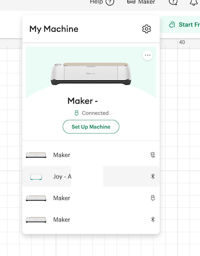
  11. Unlocking a locked/deactivated e-waste Cricut Maker13
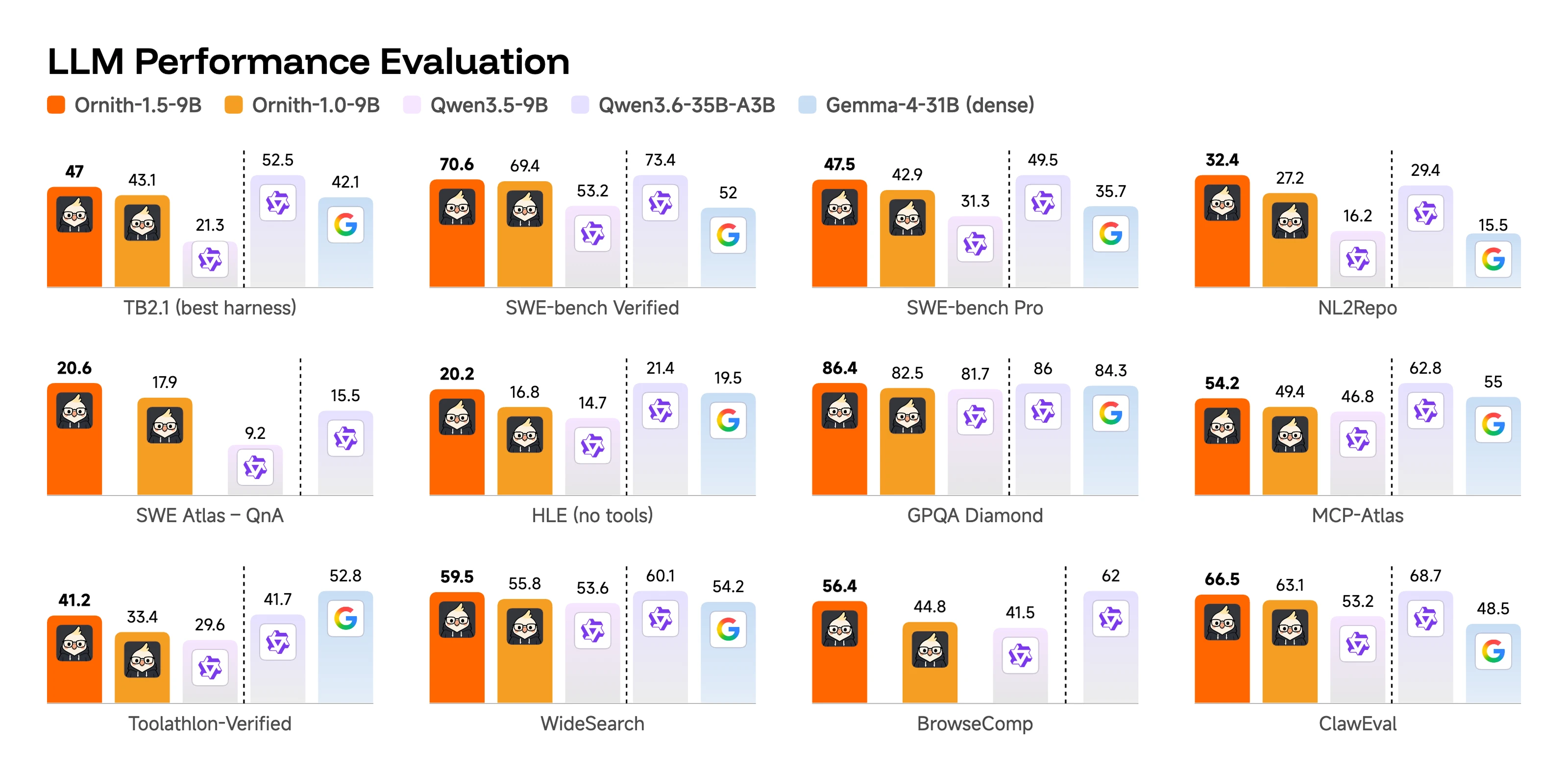
  12. Ornith-1.5: From Self-Scaffolding to Self-Improvement14
  13. Police officer used Flock cameras to track estranged wife 717 times15
  14. Opus 5.0 drives incoherence into the stratosphere16
  15. Show HN: Automatically detect and patch walking-dead states in Sierra games17
  16. Extensible Software in the age of LLMs18
  17. Bun 1.4 Rust rewrite is not looking good?19
  18. How Kubernetes Probes Work20
  19. Go 1.2721
  20. Cerebras CS-422
  21. Palomar: A registry of Lean verified mathematics23
  22. Feature Request: Support AGENTS.md24
  23. Moderna reports first positive Phase 3 for mRNA neoantigen therapy in melanoma25
  24. Civic Hygiene – avoid building technologies that could be used by a police state (2013)26
  25. Mathematics in the age of AI27
  26. Air Theremin – A browser theremin you play by waving at your webcam28
  27. Devices with GrapheneOS support should be available in 202729
  28. Google has stopped pushing Git tags for some Android source code29
  29. Casio F-B100W-1A29
  30. Meta's blockbuster trial draws parallels to big tobacco29
The Daily Front Page 2 of 30
Wednesday, August 19, 2026 The Daily Front No. #260819 — The Local-First Desk
article

OpenLogi

by amatheus·▲ 1,545 points·409 comments·openlogi.org ↗
No account, no telemetry.

A local-first alternative to Logitech Options+, written in Rust. Remap buttons, drive DPI and SmartShift over HID++. No account, no telemetry.

Download

The OpenLogi app remapping an MX Master 4's buttons over HID++

Click a button, bind an action.

The center of the app, working right here: a mouse diagram with clickable hotspots and a per-button action picker. Choose a hotspot, then bind any of the built-in actions.

schema_version = 2
selected_device = "2b042"
 
[devices.2b042.bindings]
MiddleClick   = "MissionControl"
DpiToggle     = "CycleDpiPresets"
Thumbwheel    = "VolumeUp"
Forward       = "BrowserForward"
Back          = "BrowserBack"
GestureButton = "AppExpose"

Writes straight to config.toml, the file you own.

Everything Options+ does, without the account.

OpenLogi drives your mouse over HID++ directly: buttons, DPI and SmartShift, from a native app that never phones home.

Remap any button

Bind any of 44 built-in actions to each physical button, per device. Custom shortcuts, app launchers and scripted actions too.

DPI control & presets

Set pointer resolution and cycle your own presets, written straight to the sensor over HID++.

SmartShift

Flip the wheel between ratchet and free-spin, or let it switch automatically by scroll speed.

Per-app profiles

Per-application overlays that switch the moment your focused app does. Ships in a later release.

Bolt, Unifying, Lightspeed, Bluetooth or wired

Reach devices over a Logi Bolt, Unifying or Lightspeed receiver, a direct Bluetooth pairing, or a USB cable. No receiver required.

Live device view

A carousel of paired devices with battery percentage and charge state for everything online.

Nothing between your mouse and your machine.

No account, no telemetry, no cloud. Bindings live in a plain TOML file you own, and every change goes straight to the device over HID++.

Up and running in a minute.

Signed builds for macOS, Linux and Windows. Pick your platform below. Step-by-step setup lives in the docs.

macOS

brew install --cask openlogi

Download .dmg

Homebrew is recommended, or grab the signed .dmg for Apple silicon or Intel.

Linux

Download .deb

Packages for amd64 and arm64, with .rpm and Arch .pkg.tar.zst builds also available.

Windows

Download .msi

The newest port: signed x86_64 and arm64 installers, validated on Windows 11.

Quit Logi Options+ before launching: the two fight over HID++ access, and only one app can own a receiver at a time. On Linux, the same applies to Solaar.

Things you might ask.

Something else? Ask in Telegram or open a GitHub issue.

Will OpenLogi support Logitech Flow?

It's on the roadmap, at the far end: a cross-computer pointer and clipboard bridge is a very large feature. The half that lives in the protocol already ships. OpenLogi drives Easy-Switch host switching over HID++ (0x1814/0x1815), and paired mice follow the keyboard when it switches hosts. If the rest lands, it will be opt-in and local-network only.

Can I pair a new device from OpenLogi?

Bolt pairing ships in the GUI, and Unifying and Lightspeed pairing is in progress. Until it lands, pair once with Logitech's tool or Solaar; OpenLogi drives the device from then on.

Can I import my Options+ settings?

Not yet, though an importer is in progress. In the meantime, bindings are a short TOML file you can rebuild in minutes, and unlike Options+ they stay in one portable, hand-editable file.

Why does macOS ask for Accessibility permission?

OpenLogi remaps the side buttons (Back, Forward, middle click) through a CGEventTap, and macOS puts event taps behind the Accessibility permission. The HID++ paths (gesture button, thumb wheel, DPI, SmartShift) don't need it.

How do updates work?

Only when you ask. The in-app update check is opt-in and off by default; new builds come from Homebrew (brew upgrade --cask openlogi) or the signed installers on the releases page.

Do my bindings move to another machine?

Copy the TOML file. Devices are keyed by physical identity (receiver serial and slot, or the device's own serial), so the same mouse keeps its bindings wherever the file goes. Built-in sync may come one day, but it's hard to square with the no-account principle.

The Daily Front Page 3 of 30
Wednesday, August 19, 2026 The Daily Front No. #260819 — A Balloon, a Domain, a Borderless Mess
article

A joke domain purchase turned in geopolitical warfare

by kareiva·▲ 862 points·132 comments·sprocketfox.io ↗
Strap in, this story involves a cheese fortune teller, the department of war, and nearly every other government department in between.

Strap in, this story involves a cheese fortune teller, the department of war, and nearly every other government department in between.

In 2017 (I think?) I was introduced to weather balloon hunting by Mark VK5QI. At the time the Australian balloon chasing community was small. Only Melbourne and Adelaide radiosondes (the transmitter on weather balloons) were being tracked on a website called Habhub - high altitude ballooning hub. This site was designed for amateur balloons and not meteorological weather balloons.

Over time more and more radiosondes were tracked on Habhub and eventually Habhub admins introduced a default filter that removed weather balloons by default. A query parameter could be added to the URL to remove the filter and on 12th of May 2018 sondehub.org registered with a single purpose - a URL redirect to Habhub with a radiosonde specific filter. To be clear - this was more of a joke than a decision to run a radiosonde tracking service. You’d go to sondehub.org and it would redirect you to habhub.org. That was it.

However Habhub was never designed for so many unique balloons each day. By July we decided to start proxying radiosonde ingestion data through SondeHub. This allowed us to capture more data as well (no longer rate limiting our selves). This went to a seperate OpenSearch cluster, however at this stage we didn’t use or expose this data. I was using this more as a toy - to play around with different Amazon Web Services (AWS) services and analytics platforms.

By 2019 the Habhub servers were really struggling - aprs.fi as well. We realised that we needed to run our own service and our initial plan was that we would build new APIs, and eventually new frontend. We then started getting information requests from government agencies regarding radiosonde data. For example we received a request regarding an insurance claim about a radiosondes hitting a horse, causing it to bolt through a fence. One of the reasons for this is because unlike official software at the time, our system tracked the radiosondes all the way to the ground.

Also in 2019 we detected a drop in radiosonde launches. This lined up with the GPS rollover date - we thought our software was broken however it turned out to be issues with Vaisala’s equipment which prevented launches from occuring. Funnily enough our software handled the rollover ok.

In 2020/2021 we ended up doing was building backwards compatible APIs for the Habhub frontend and started testing the Habhub frontend pointed at our backend. It mostly worked. We started receiving all the data rather than just partial data and providing open access to our data via S3. We even started running our own predictor - which is used by my entities today.

With our own predictor running Mark developed a system we call reverse predictions. This is where we take data from an already launched radiosonde and use the wind model to run the predictor backwards which determines a rough the launch location prediction. It works extremely well. We could detect a bunch of radiosonde launch sites that were poorly otherwise documented along with start assigning balloons to launch sites.

Our first taste of dealing with the military

Then in 2021 we received an email

sensitive/military/… installation. As such, we really prefer that it is not explicitly marked on any map.

The thing is though that wind data isn’t just used for predicting the weather. It’s also used to calculate artillery ranging. What we had started doing is accidentally mapping out artillery sites. We decided to keep reverse predictions but we delete launch sites on genuine requests.

The reverse prediction system has also detected many number of military vessels in the ocean.

Lots more development happened on SondeHub with features like websockets and MQTT for live feeds. We disconnected Habhub backend from our proxy and with grant funding from ARDC we were able to setup a prototype amateur high altitude balloon version of SondeHub.

Eventually Habhub was shutdown due to a lack of maintenance and we rushed together to migrate what we could to SondeHub.

$439,000 missile vs party balloon

All was going fine until the 2023 “China spy balloon” incident. SondeHub had a lot more traffic - but our architecture made it fairly manageable.

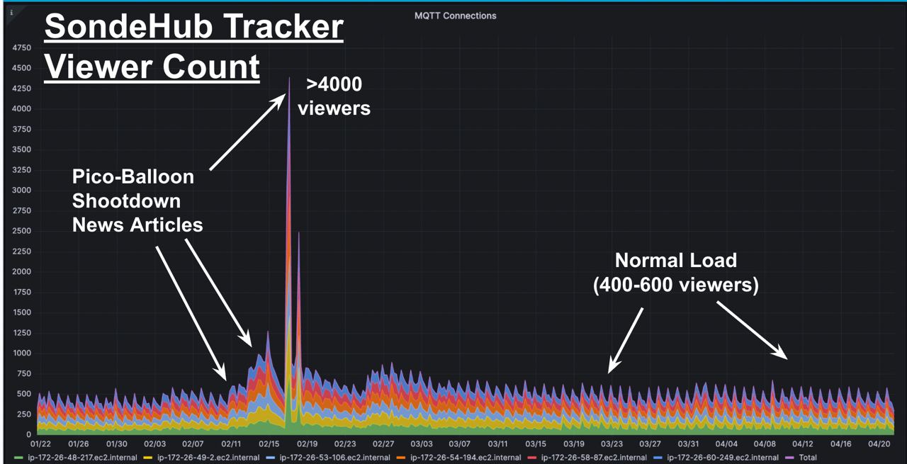
Then Feb 11th 2023 the US allegedly used AIM-9X Sidewinder to shot down an amateur radio balloon. That morning I woke to high usage alarms in my inbox. SondeHub had been linked to on the Washington Post. Our site managed to handled the extra traffic reasonably well.

Plot of websocket users spiking several times

Since then we’ve many support requests from .mil and .gov addresses. We’ve also had requests from aviation industry / air control towers.

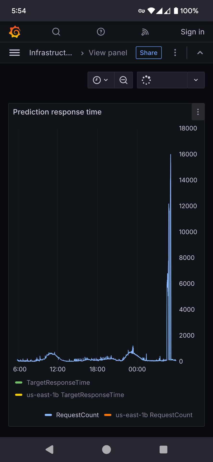
In Dec 2024 - alarms in my inbox again. This time getting alarms for predictions. Someone decided to smash our api. This seemingly starts happening every week.

rafana plot of request count spiking on the predictor

Full scale invasion

We turn on logging. The requests coming from a single IP. We had some suspicions that a private company was using our backend to generate predictions. We poke their website to see - sure enough they are - an angry email to them. However they weren’t the problem.

We ask some people.

Messages on telegram suggesting that it might be russia DDOSing us because Ukranians might be using it to help drone operations

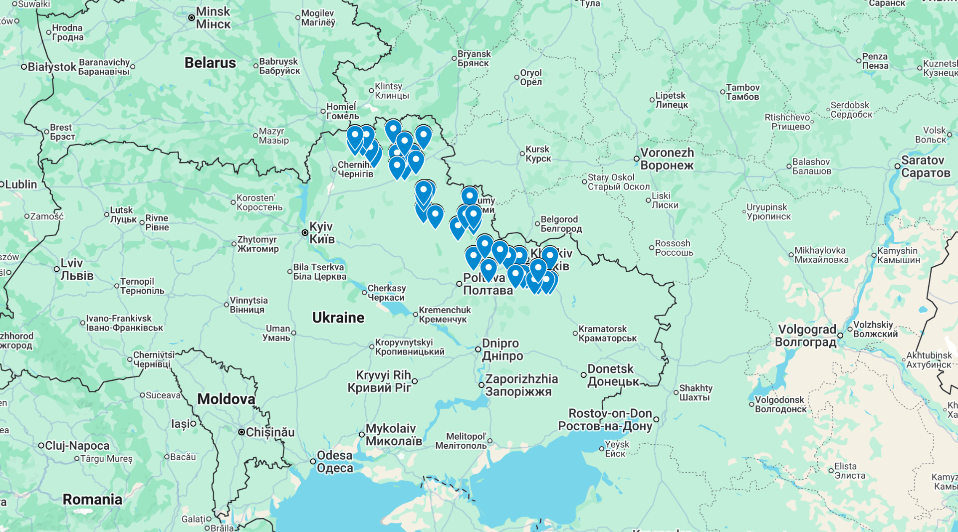
Lol. Totally not the case. Right? Probably just an AI LLM bot scrapper gone crazy. Lets plot some predictions.

Points on a map near the Ukraine/Russian border

Note that the precision of these points has been intentionally been reduced. This data is also significantly old and does not show the entire dataset. This blog post has been delayed until balloon warfare was more common knowledge.

Fuck. And Fuck Russia.

(for time travellers and people in the future - in 2022 started a “special military operation” - aka a full scale invasion into Ukraine. The war continues at time of writing. Fuck Russia)

Suddenly my mind was filled with ethic and legal questions. We also suspected they aren’t using the API correctly. However we didn’t know how to get in contact.

We did eventually got some messages out via a contact

“We work with mHAB’s as you know, but some other groups likely fly fixed-wing and use Sondehub to help them “surf” the sky to target areas.

“Sent this in Ukrainian to a few milchats and will see what turns up: “I wish everyone good health. If anyone knows of a deep strike team that uses a python script with some open source wind forecasting engine, please contact me directly. They are causing numerous problems with queries, which can lead to them being blocked and they need to take action to be able to continue using the prediction system.””

I also quickly rushed together a docker compose file so anyone could quickly run their own predictor that wasn’t reliant on us.

Meanwhile (and you might have noticed me asking for AWS help on fedi) we contacted AWS as the source IP was from an AWS network. It was very important however to make sure the AWS support did not shutdown access.

Our messaging included:

It is incredibly important that the http request data is not distributed. It is also important that the source AWS account is not blocked, rate limited or terminated - loss of life could occur.

Something that I thought I’d never have to write in support emails. The messaging was important because I did not want the service cut off, and I did not want the data to reveal launch sites.

After a bit of waiting we received:

AWS reached out to me that a lambda function of mine was flagged for potentially scraping api.v2.sondehub.org and they told me to reach out to you to get this resolved.

We emailed back and forth and provided documentation on how to run the predictor locally.

Office of the Secretary of War (Intelligence and Security)

In 2025 we received a request for data from the “Office of the Secretary of War (Intelligence and Security)” (US). Generally if there’s mutual community benefit we’ll find, process and release the data for free. However given this is was the Department of War and no expected community benefit we decided they should pay for the data. I was hesitant even working with them, as I don’t really want to help military, let alone the US - but since our data is public if we didn’t do it someone else probably would. So my reasoning shifted to, may as well extract some funds to pay for SondeHub infrastructure at the very least.

An invoice was created and sent through - but never paid or followed up on. I have no idea why they were requesting the data or what it was about.

Other tidbits along the way

It hasn’t just been the military that we get emails from. Occasionally citizens who find radiosondes end up contacting us (often we don’t know how they even find us), along with a range of other organisations.

National Transportation Safety Board (US)

In September 2025 the NTSB contacted us. My first reaction was to search for news stories.

do you have information on any balloons in the Utah are between 1200 and 1300 UTC on 10/16/2025

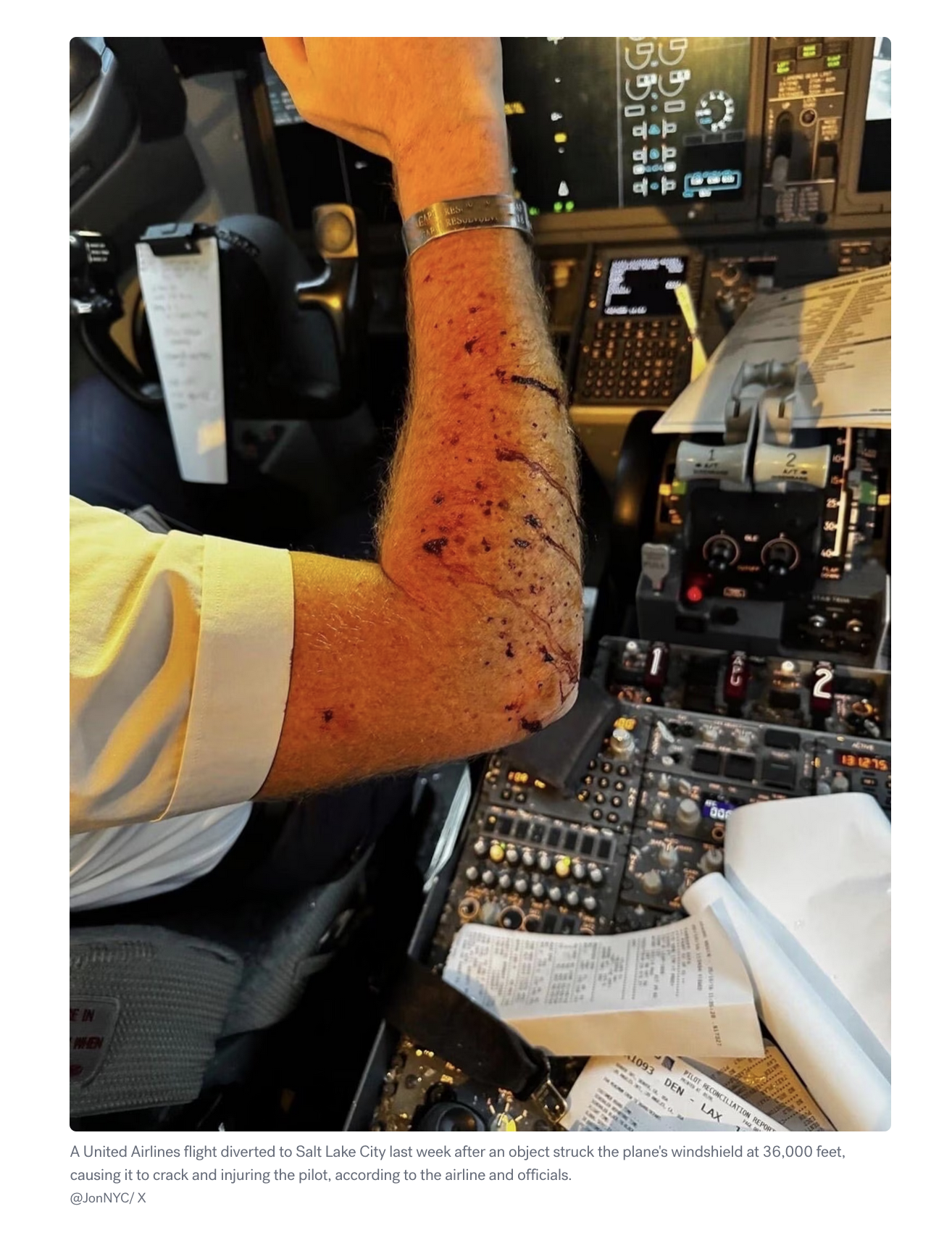
We provided our data but also started hearing some rumours about a possible plane / weather balloon collision that was reported via ACARS. While none of the balloons tracked by SondeHub lined up, we did forward some information that a Windborne balloon was in the area. Windborne later confirmed this was the likely collision and have made several changes to their system to prevent future issues.

Plane with a cracked window and damage around the edge of the window

Pilot with cut arm from glass shards

We have a number for you to call when you’re ready to copy

Please contact us as soon as practicable with more information… Contact our Operations Manager at

This was a really strange interaction for us. A tower(?) operations supervisor was requesting information about balloons in the area. The balloons in question were meteorological weather balloons. Not launched by amateurs. We had to explain that they are normally scheduled, not controlled, and fall (probably, not a lawyer) within Part 101.D of FAA regs. Along with that we didn’t have contacts or registration details of these launches.

We have a lot of Aircraft in the sky that don’t want to get too close to one of these balloons! Is there any way to coordinate more directly with the controlling entity, or to have them give us mission details and contact information ahead of time? It sounds like you guys have a big operation, I don’t know if this is a one off event or if you have systems in place to communicate these things

Explaining to the FAA that weather balloons exist wasn’t on my bingo card.

Hit and run

On 2/5 around 8pm was there a balloon located in Anamosa Iowa?

Facebook post showing the incident and building damage

Someone recovered a radiosonde from a property but ran into a building along the way. They left without leaving a note. The property owner contacted us for help to locate the person.

Jam, tasty tasty jam

There’s a great site that uses ADSB data to track GPS jamming called gpsjam.org. We’ve also been detecting not only a lot of GPS jamming but also GPS spoofing. I always find the patterns interesting. I’ve been presuming that the pattern is either for making the impacted targets easier to identify or to crash the vehicle in a specific way?

screenshot showing a perfect circle for the track of a radiosonde

Zoomed out view of the above showing the large distance the gps had shifted

The cheese fortune teller and other job titles we’ve seen over the years

Probably the most interesting job title we’ve had the pleasure of reading in an email is from Jennifer Billock, Freelance Writer and Author, Certified Tea Specialist, Cheese Fortune Teller. Jennifer wrote an article for STNDRDS about weather balloons which is outside our usual places of exposure.

During this time we’ve seen many job titles and subjects, I’ve started collecting them.

  • [SEC=🌶️🌶️🌶️]
  • Naval Air Warfare Center – Aircraft Division Maritime Patrol and Reconnaissance Aircraft (MPRA) Program
  • Acquisition Program Manager Integrated Processes Branch HQ AFRL/XPOP
  • Upper Air Quality Assurance Meteorologist Observing Systems & Operations, Data & Digital Group
  • Senior Advisor for Safety and Quality
  • Meteorologist Weather Forecast Office
  • Manager Upper Air Network
  • General Manager Observing Systems and Operations and Chief Engineer
  • Meteorologist National Weather Service
  • Field Research Manager, Center for Western Weather and Water Extremes
  • Video Journalist, Visual Investigations - NY Times
  • Senior Meteorologist, National Transportation Safety Board
  • Operations Supervisor U.S. Department of Transportation/FAA
  • STNDRDS Freelance Writer and Author, Certified Tea Specialist, Cheese Fortune Teller
  • Meteorológiai fejlesztő (met.hu)
  • SUNY Oswego Lab Technician Atmospheric and Geological Science
  • SpaceBalloon Project
  • Any many more

The weird

Most organisation and vendors are willing to work with us. This is because chasing radiosondes removes them from the environment and promotes citizen science. I asked “Meteolabor AG” for one of their radiosondes so that we could confirm compatibility. This is what I received back.

Official response from Meteolabor AG: For strategic reasons, we do not provide any data or sample devices. Our transmitters shut down after a certain period of time, at the latest when the battery capacity is exhausted. This is due, among other things, to strategic considerations.

We are aware of the so-called waste problem.


Personal comment: I would personally like to draw attention to military activities, particularly in the Middle East, which result in significantly (exponentially) more waste and toxic substances being released into the atmosphere and left lying around in the environment – or entering the food and water cycles

In addition to military operations, countless “missions” are currently being flown over Europe with the aim of leaving “contrails” in the sky [rather “chemtrails”]. I know their purpose; I know what NetZero is supposed to achieve, and what decarbonization and CO2 reduction are intended to accomplish. I am well-informed about the climate hoax.

Start there! The people to talk to are politicians, NGOs, and very wealthy old white men.

Which is… certainly something.

Onwards

I hope you liked this selection of SondeHub chaos. I haven’t included every interaction we’ve received over the years, so there might be a part 2 to this post in the future.

The Daily Front Page 4 of 30
Wednesday, August 19, 2026 The Daily Front No. #260819 — The Router Joins the Tollbooth
article

OpenRouter is joining Stripe

by rvz·▲ 802 points·409 comments·openrouter.ai ↗
We now process 10+ trillion tokens per day from 400+ AI models.

OpenRouter is Joining Stripe

Today, we are excited to announce that we are joining forces with Stripe, to power the next wave of GDP growth globally.

OpenRouter is the first and largest model marketplace and gateway. We are the best way to discover and use any AI model, with one interface, broad provider choice, model-agnostic observability, cost management, and routing that improves price, performance, and uptime. We now process 10+ trillion tokens per day from 400+ AI models for a community of over 10 million developers and companies. Since our founding, we have seen at least 10x growth in inference volume every year.

We want to explain why we made the decision to join forces with Stripe and what it means for the millions of developers and companies that build on us.

What this means for our users

OpenRouter will continue to operate as it is: same mission, same name, same product, same roadmap. If you build on OpenRouter today, nothing about your integration changes.

OpenRouter exists to give users every model on equal footing, provide open signals about how they’re used in the market, help developers orchestrate them together, and make them observable and manageable at scale. That commitment is core to how we operate, and it doesn’t bend to any model, any provider, or any parent company. It also extends to a growing ecosystem of inference-adjacent services, including AI-native web search, context management, and more to come.

Routing decisions will remain driven by one thing: what’s best for you, the user.

Our mission

We started OpenRouter in early 2023 on a simple belief: intelligence will be multi-model. No single model will win every task, and the frontier will move rapidly. That freedom is critical infrastructure for the industry. AI is too important for its future to be decided by whichever single model gets embedded first. AI has become the single largest driver of economic growth in the US, and inference is quickly becoming the largest line item for every company.

We envision a healthy AI ecosystem where many models thrive, where AI neurodiversity is a strength, where a lab or an inference provider with a breakthrough can reach millions of developers, and where no single model becomes the default by inertia.

Our mission is to realize this future, and it’s more important than anything else. The opportunity with Stripe allows us to accelerate it together.

Why Stripe?

There are few companies on earth we would have considered selling to; our mission, our neutrality, and our lead in the market make the story for independence strong. We would only join a company if we thought we could do more together, faster, without compromising any of them.

Stripe is that company. They are the best financial infrastructure platform in the world. Their API set the standard that developer products, including ours, have been measured against ever since. This is a combination of two platforms that developers choose on merit, with cultures focused on quality, scale, and commitment to builders, and that will remain essential in a post-AGI economy.

For years, OpenRouter has been called “Stripe for LLMs.” Both companies share common DNA: we abstract complex infrastructure and market dynamics into delightful APIs, and we obsess over the developer and user on the other side of it. Businesses trust Stripe to optimize every part of their revenue stack, across payment methods, authorization, fraud, and more. Builders, customers, model labs, and providers trust OpenRouter to run a neutral, reliable layer across a fast-moving ecosystem.

Stripe brings a large customer network, data on how internet businesses grow, and years of experience running trusted global infrastructure. There is also no one better at managing fraud and abuse, something we believe will only become more challenging for AI companies to address. We can now serve developers at a pace we couldn’t reach alone.

What’s next

To our customers: Thank you. We’re honored to be part of your journey, and we’re just getting started. OpenRouter’s product, mission, and current commitments remain unchanged. Joining Stripe helps us pursue them faster, and our ability to support you will only improve.

To our employees: We firmly believe that the next few years will be the most important time of our lives, and the most important for our mission. We are so grateful to have the privilege of being alive during this transformation for the world, and that I get to do it with you. You are some of the most brilliant, creative, curious, and determined people there are, and we’re excited to grow our team for an even greater global impact.

To everyone else who believes in our mission: come join us. Fitting into a role isn’t as important as having our values: curiosity, rigor, agency, and transparency. AI will transform the way companies are organized, and OpenRouter will innovate significantly here. And as we grow, we will relentlessly aim to preserve the velocity, agility, efficiency, and talent density of the 90-person startup that we are today.

— Alex, Chris, Louis, and the OpenRouter team

The transaction is subject to customary closing conditions. We expect to close in the coming weeks.

The Daily Front Page 5 of 30
Wednesday, August 19, 2026 The Daily Front No. #260819 — Work, Well-Being, and the Commute
article

Remote workers report the highest well-being in study of 7,700 employees

by downbad_·▲ 559 points·283 comments·colorado.edu ↗
Employees who worked fully remotely reported the highest levels of well-being.

Woman working from her dining room table with two computers

For years, many employers have worried that work-from-home arrangements leave employees isolated, disconnected from coworkers and more likely to leave their jobs.

But according to a new study, remote workers are doing better than many employers realize.

Researchers analyzed survey data from 7,704 employees at a large healthcare organization. One pattern stood out: Employees who worked fully remotely reported the highest levels of well-being, while those who worked entirely onsite reported the lowest. The study also found little evidence that remote workers felt less connected to colleagues or workplace culture.

"This suggests you let people work remotely if they want to work remotely," said Stefanie Johnson, professor of organizational leadership and information analytics at the Leeds School of Business and co-author of the study, published in July 2026 in the journal Frontiers in Psychology. "Taking away people's choice of how they work is probably not going to help them in terms of their well-being."

Stefanie Johnson

Stefanie Johnson

As companies continue to debate remote work, many leaders worry that employees need to be in the office to stay connected, work well together and remain committed to their organization. Johnson said the research doesn't always support those concerns.

"The data from our study and others suggest remote and hybrid work result in better outcomes than return-to-office mandates," she said. "Leaders are not making decisions based on data. I think they are just returning to what they are used to."

Rethinking remote work

Johnson, who co-authored the study with Alyssa Lezcano, Stephanie Zajac and Courtney Holladay of the MD Anderson Leadership Institute in Houston, said the results surprised her. She thought employees who split their time between home and the office might have the best of both worlds.

"I actually thought you would be happiest if you were part time out of the office," she said. "Then every once in a while you get to see people, get that human connection."

Instead, the data pointed in a different direction.

Among employees in the study, well-being was highest for fully remote workers, followed by hybrid employees and then onsite workers.

The findings also cast doubt on one of the main arguments for bringing employees back to the office: that people need to be together in person to feel connected.

Employees in the study were asked to describe their organization's culture in a handful of words. Remote workers were slightly more likely than their hybrid and onsite peers to use words associated with teamwork, inclusion and support.

"People who are remote actually said more things that indicated they had more positive connections, even though they were remote," Johnson said.

Still, Johnson said face-to-face interaction can play an important role in helping coworkers build relationships, especially if they are just starting out in their careers.

"Remote works better after you know people," she said. "So there is still a benefit of having some face time."

Staying power

The researchers also examined employee turnover one year after the survey was completed.

They found that employees with higher well-being were less likely to leave the organization. Work location itself was not a strong direct predictor of turnover. Instead, remote work was associated with higher well-being, which in turn was associated with lower turnover.

"It makes sense. If you have higher well-being, you're less likely to leave your job," Johnson said.

Participants completed the workplace survey in 2023, and researchers compared those responses with actual turnover records one year later. Of the employees surveyed, roughly half worked onsite, with the remainder split between hybrid and fully remote arrangements.

Flexibility matters

The study did not explore why remote workers reported higher well-being, but Johnson points to a growing body of research on autonomy and flexibility.

One explanation is that remote workers have greater control over their work setup and daily schedule, she said.

"If you have control over your environment, you tend to have more positive outcomes," she said.

Working from home can also eliminate many everyday stressors.

"Spending a lot of time in traffic is negatively related to well-being," Johnson said. "There are so many little stressors associated with being in the office."

Those stressors can include arranging child care, hiring help for pets or managing the logistics of getting to and from work, she said.

Johnson said the study points to a broader lesson for employers navigating return-to-office debates. Rather than focusing only on where employees work, organizations may get better results by investing in employee well-being.

"I think flexibility is here to stay," she said.

The Daily Front Page 6 of 30
Wednesday, August 19, 2026 The Daily Front No. #260819 — Finding the Island
article

Geolocating a random island using geometry and CUDA programming

by yassa9·▲ 463 points·78 comments·yassa9.github.io ↗
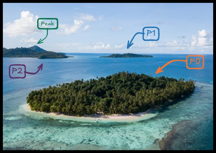
This is a photo of a resort located on an island.

I'm writing this page as a writeup for this challenge gralhix 004 made by Sofia Santos | Gralhix.

You can view, clone and locally try all code files and the final report with all instructions here at github.


Task briefing:

main

This is a photo of a resort located on an island.

a) What is the name of the resort?
b) What are the coordinates of the island?
c) In which cardinal direction was the camera facing when the photo was taken?

In my opinion, solving this challenge with google lens is wasting a fun opportunity, so decided to solve it with math and programming.


a] Metadata

Of course, first thing u look for is the metadata. Ran that on my linux void:

> exiftool main.png

File Type                       : WEBP (lossless)
MIME Type                       : image/webp
Image Width                     : 736
Image Height                    : 515

As expected, nothing useful here. No EXIF, no GPS, no camera make or model.


b] Building the fingerprint

01_00

U can see from the img, there are 3 landmasses:

  • P0: the islet itself,
  • P1: the right island,
  • P2: the left front island ( having mountain peak )

I couldnt make a correct perspective model of birdview of this image, as clearly the image is taken by a drone and cant estimate the elevation at all (and not found in the metadata).

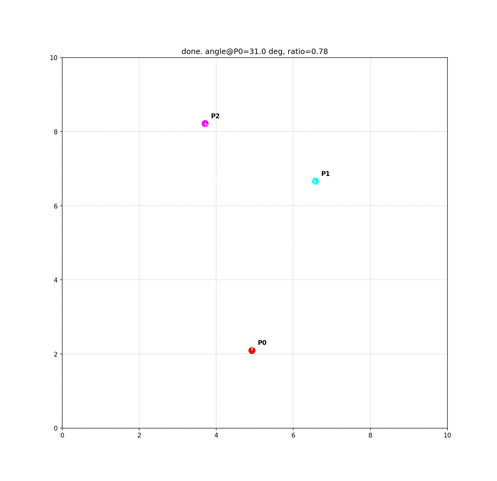
So I had to estimate that by intuition, I just want the relative distances between the 3 islands and angles of that triangle.

01_01

I built a small click GUI 01_triangle_gui.py that records pixel coordinates for each point in order and computes the triangle's geometry.

Since clicking exact centers by eye isn't perfectly precise, I added a ±20% tolerance band around both values when searching.


c] SEARCH

With the fingerprint locked in, the next step is checking every real landmass on Earth against it !

I used OpenStreetMap's split land polygon set as the dataset land-polygons-split-4326, full global coastline vectors in WGS84 which has size of 882 MB.

I created heuristic filters (all by just intuition and non tangible proofs), spent days (yea full days) tweaking values and tons of trial and error 😭 untill I got this working filters recipe.

01] Tropical latitude bounding box

$$ -30° \le latitude \le 30° $$

the islet in the photo reads as tropical, so I decided that anything outside the tropics is thrown out immediately, before doing any expensive geometry work.

Exactly 141,131 land polygons survive that band filter.

02] Local density filter

$$ N_{5\text{km}}(p) \le 10 $$

$ N_{5\text{km}}(p) $ counts how many other centroids fall within 5km of point (p). Cap is 10: if an islet has more than 10 neighbors that close, it's sitting in a dense reef field, a crowded coastline or a archipelago clutter, not a small isolated 3-4 island group like the photo shows.

This dropped candidates down to 51,576.

03] Clustering

For every surviving point, find every other point within 20km (heuristic, by eye from the image). If it has at least 2 neighbors that close (3 points total), it's a cluster. Points with no cluster of 3+ nearby are dropped, they can't form a triangle at all.

tree = cKDTree(f_coords)
neigh = tree.query_ball_point(
                            f_coords, 
                            CLUSTER_RADIUS_KM / 111.0)
clusters = set(tuple(sorted(n)) for n in neigh if len(n) >= 3)

$$ \left|\{q : \text{dist}(p,q) \le 20\,\text{km}\}\right| \ge 3 $$

That collapses down to 23,500 clusters.

04] Generating Triplets

For every cluster, every combination of 3 points inside it becomes a candidate triangle. That's $ C(n, 3) $, which explodes fast for big clusters, for example: a cluster of 60 points already gives 34,220 triples on its own. So each cluster gets capped at 60 points first, sampled by size, not randomly.

$$ \binom{n}{3} = \frac{n(n-1)(n-2)}{6} $$

def stratified_sample(idx_arr, area_arr, cap):
    order = np.argsort(area_arr[idx_arr])
    n_small = cap // 3
    n_large = cap // 3
    n_mid = cap - n_small - n_large
    mid_start = max(0, (len(idx_arr) - n_large - n_mid) // 2)
    keep = np.unique(np.concatenate([
        order[:n_small], 
        order[-n_large:], 
        order[mid_start:mid_start + n_mid],
    ]))
    return idx_arr[keep]

def gen_cluster_triples(idx_arr):
    local = np.array(list(
                itertools.combinations(range(len(idx_arr)), 3)), 
                dtype=np.int64)
    return idx_arr[local]

The sampling takes a third small islands, a third large, a third from the middle of the size distribution, instead of the full cluster or a random cut.

23,500 clusters produce 80,690,777 triples total !!

05] Matching, on the GPU

I gave every triple one CUDA thread. Each thread sorts its 3 points by land area to pick out P0 (smallest, the resort islet), then uses the winding direction of the other two to assign P1 and P2:

long long i = blockIdx.x * (long long)blockDim.x + threadIdx.x;
if (i >= n_triples) return;

int pos[3] = {0, 1, 2};
for (int a1 = 1; a1 < 3; a1++) 
{
    int key = pos[a1];
    double keyval = a[key];
    int j = a1 - 1;
    while (j >= 0 && a[pos[j]] > keyval) 
    {
        pos[j + 1] = pos[j];
        j--;
    }
    pos[j + 1] = key;
}

P1 vs P2 comes from a 2D cross product, no branching on which cluster the triple came from, just the sign:

$$ \text{cross} = x_a y_b - x_b y_a $$ $$ P1 = \begin{cases} a & \text{cross} > 0 \\ b & \text{cross} \le 0 \end{cases} $$

Walk from P0 to a, then to b. If cross > 0, that's a left turn (counterclockwise). If cross < 0, it's a right turn (clockwise). It's the same sign trick used to tell if 3 points curve one way or the other.

then angle at P0 and the distance ratio, same formulas as the fingerprint step, computed independently by every thread:

$$ \theta_0 = \arccos\left(\frac{\vec{d_1} \cdot \vec{d_2}}{|\vec{d_1}||\vec{d_2}|}\right), \qquad r = \frac{|\vec{d_1}|}{|\vec{d_2}|} $$

A triple survives if angle, ratio, P0's size, the separation between P0 and P1, and both side lengths all land inside the fingerprint's tolerance windows. Threads that pass write their result into a shared output array using an atomic counter, so two threads finishing at the same time never overwrite each other:

if (hit) 
{
    unsigned long long slot = atomicAdd(out_count, 1ULL);
    out_p0[slot] = p0idx;
    out_p1[slot] = p1idx;
    out_p2[slot] = p2idx;
}

Now printed in the CLI directly from the kernel:

gpu: NVIDIA GeForce RTX 3050 (sm_86)
vram used: 5169 MB
kernel time: 204.1 ms

80.7 million triples go in, one thread each, in parallel. 158,784 pass the mask.

06] Dedup

Since same physical triple can get hit by multiple GPU threads if it belonged to more than one overlapping cluster, so raw matches get collapsed by identity first:

seen = set()
uniq = []
for i in range(len(p0_all)):
    key = (p0_all[i], p1_all[i], p2_all[i])
    if key not in seen:
        seen.add(key)
        uniq.append(i)

8,915 unique triples after dedup.

07] The Open Rectangle

02_00

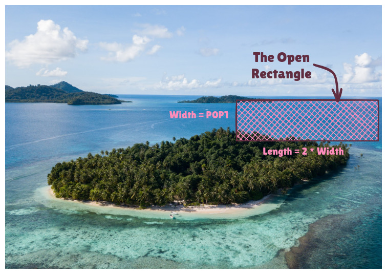
Every surviving triple gets one more test: is the space next to it actually open water, like the photo shows ? A rectangle gets built along the P0→P1 edge, on whichever side P2 is not on, then checked against the land dataset for anything else sitting inside it.

width = np.hypot(x1, y1)
u = np.array([x1, y1]) / width
v = np.array([-u[1], u[0]])

# p2 sits on the +v side by construction, 
# so the check goes on -v
length = 2 * width
corners_local = [
    (0, 0), (x1, y1),
    (x1 - v[0]*length, y1 - v[1]*length),
    (-v[0]*length, -v[1]*length),
]

If anything other than the 3 candidate islands themselves intersects that rectangle, the candidate is dropped. Land sitting there means it's not the open, unobstructed water the photo actually shows.

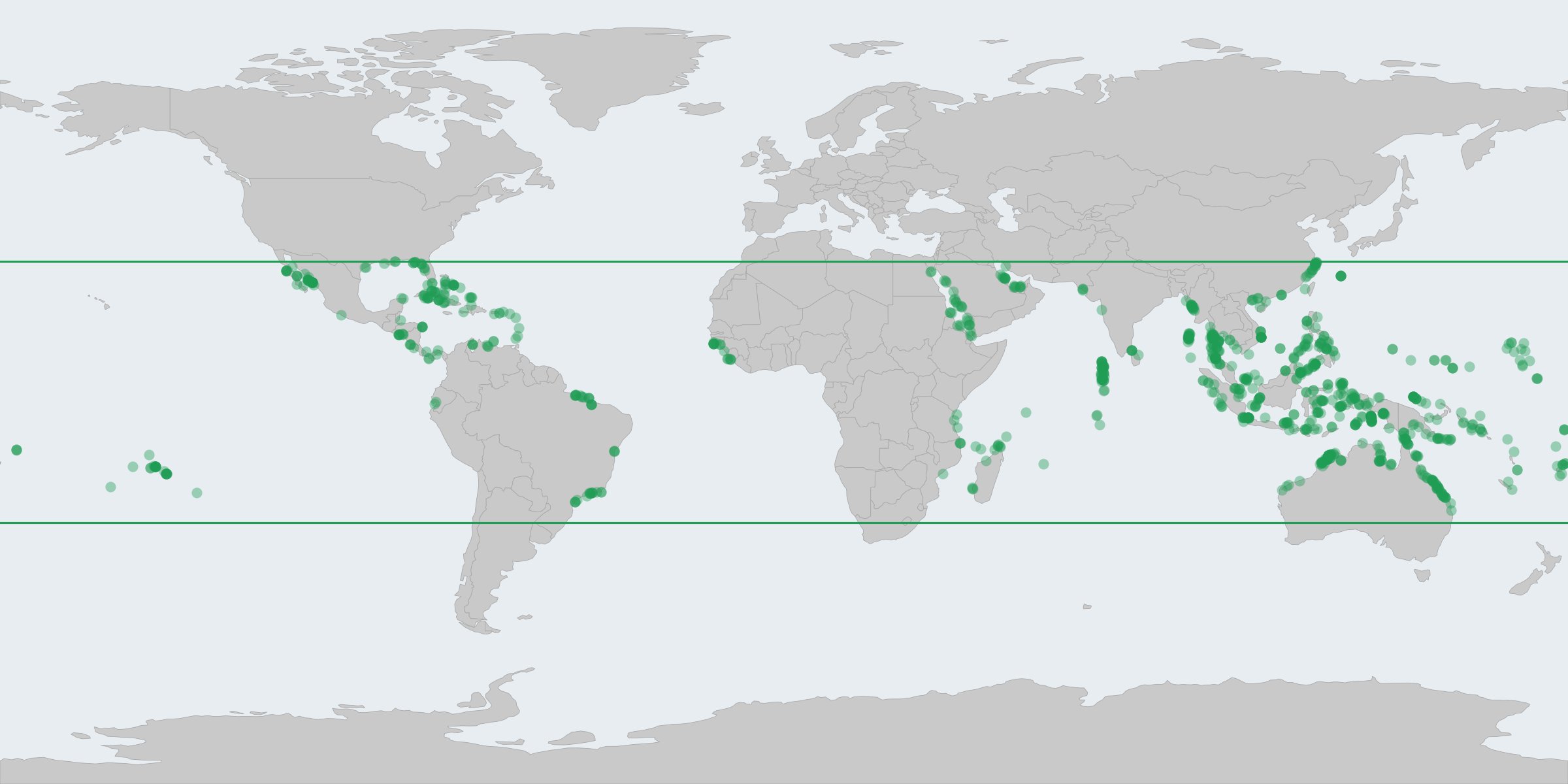
8,915 unique triples down to 948.

and below is the map of places of the 948 candidates.

02_01


d] Coral Cay Shape Check

In this stage, we look only at P0, the resort islet, and check whether its shape actually looks like a coral cay.

1] Compactness, how close to a circle the shape is:

Polsby Popper Score: $$ PP = \frac{4\pi \cdot \text{area}}{\text{perimeter}^2} $$

def compactness(row):
    return (4 * np.pi * row.area_km2) / (row.perim_km ** 2 + 1e-12)

03_00

1.0 is a perfect circle, lower means a more jagged or elongated outline. Coral cays tend to be round from wave deposition, so anything < 0.5 gets dropped.

2] Micro Cay Halo Check:

def micro_cay_count(gdf, sindex, lon, lat):
    dists_km = nearby.geometry.distance(pt) * 111.0
    mask = (dists_km > 0) 
           & (dists_km <= HALO_KM) 
           & (nearby["area_km2"].values < MICRO_KM2)
    return int(mask.sum())

We Count land fragments under 0.05 km² within 1.5km of P0 ( just heuristic ). Real reef systems scatter tiny sandbars around the main island, not just one isolated landmass (I knew that with the hardway 😭). So we need at least 1.

213/948 candidates survive both checks.


e] Oval Shape Check

Another geometric filter on P0's own polygon. Fits the minimum rotated rectangle around it and measures two ratios from that box.

def aspect_and_fill(geom):
    mrr = geom.minimum_rotated_rectangle
    coords = list(mrr.exterior.coords)
    s1 = math.hypot(coords[1][0] - coords[0][0], 
                    coords[1][1] - coords[0][1])
    s2 = math.hypot(coords[2][0] - coords[1][0], 
                    coords[2][1] - coords[1][1])
    long_side, short_side = max(s1, s2), min(s1, s2)
    return long_side / short_side, geom.area / mrr.area

Aspect ratio is long side over short side of that box:

$$ \text{aspect} = \frac{\text{long side}}{\text{short side}} \in [1.05,\ 2.2] $$

Too close to 1.0 and it's basically a perfect circle, not the slightly elongated shape in the photo. Too high are shapes too much elongated more than 2:1.

Fill ratio is how much of that bounding box the shape actually fills, and this one has an identity behind it: any ellipse fills precisely $ \pi / 4 $ of its own minimum area bounding rectangle, regardless of how stretched it is.

$$ \frac{\text{area}_{\text{ellipse}}}{\text{area}_{\text{box}}} = \frac{\pi}{4} \approx 0.785 $$

that's the theoretical ceiling for a perfectly smooth oval. Real coral cays aren't perfect ellipses, so the cutoff is set as a heuristic safe fraction of that ceiling:

$$ \text{FILL\_RATIO\_MIN} = 0.75 \times \frac{\pi}{4} \approx 0.589 $$

A shape needs to retain at least 75% of a perfect ellipse's fill to survive. Crescents, rings, and notched coastlines fall well below that, solid rounded cays don't.

137/213 candidates survive.


f] NDVI Vegetation Check

We reached the final API phase, I put it at the end, because it is network bound not compute bound.

We gonna connect to Earth Search, run by Element84, a public STAC API that indexes Sentinel-2 imagery hosted on AWS's Open Data program, free, no API key.

You can look at it https://earth-search.aws.element84.com/v1

We now check whether P0 is actually vegetated, palm cover, not bare sand or rock. It pulls the most recent low cloud Sentinel-2 scene over the point from a public STAC catalog, samples the red and near infrared bands at that exact pixel.

$$ \text{NDVI} = \frac{\text{NIR} - \text{Red}}{\text{NIR} + \text{Red}} $$

Live vegetation reflects strongly in near infrared and absorbs red light, so healthy palm cover pushes NDVI well above 0, bare sand or open water sits near 0 or negative.

04_00

You can view this image I got from this nice Geoawesome Blog.

Threshold is set at 0.6, high enough to require real tree cover, not just scattered units.

66/137 survive the NDVI check.


g] Elevation & Mountain Check

05_00

Last check before the final reveal. There are two conditions:

  • P0 itself must be low and flat, consistent with a small reef islet,
  • P2 must have real elevated terrain in the direction the camera was actually facing.

The "front" of the shot is the bisector between the bearing to P1 and the bearing to P2:

$$ \theta(P_0, P_i) = $$ $$ \text{atan2}\Big(\sin(\Delta\lambda)\cos\phi_i,\ \cos\phi_0\sin\phi_i - \sin\phi_0\cos\phi_i\cos(\Delta\lambda)\Big) $$

$$ \theta_{\text{front}} = $$ $$ \theta(P_0, P_2) + \frac{\big((\theta(P_0,P_1) - \theta(P_0,P_2) + 180) \bmod 360\big) - 180}{2} $$

That gives one heading, the direction the lens was pointed. From there, a fan of sample points gets swept ±50° around that heading, at radii from 2km out to 20km:

$$ (\text{lat}, \text{lon}) = \Big(\text{lat}_0 + \frac{r\cos\theta}{111},\ \ \text{lon}_0 + \frac{r\sin\theta}{111\cos(\text{lat}_0)}\Big) $$

Every one of those points gets sampled against real 30m Copernicus DEM tiles.

Copernicus DEM GLO-30, published by the EU's Copernicus program, hosted as free public Cloud-Optimized GeoTIFFs on AWS Open Data, no account or key needed.

For more info, you can view https://registry.opendata.aws/copernicus-dem/

Finally, those two simple heuristic conditions decide survival (yea I know, everything became heuristic haha):

$$ \text{elev}(P_0) \le 50\text{m} $$ $$ 100\text{m} \le \max_{\text{arc}}(\text{elev}) \le 500\text{m} $$

05_01

You can see from this abstract graph image, the dashed line is the camera's front bearing, the wedge is the ±50° search arc swept out to 20km for the elevation check.

26/66 survive the elevation check.

You can see the 26 survivors, all are located in southern Asia, Australia and Oceania, except one near Brazil!

05_02


h] Final Report

Finally, last stage, it just makes the final candidates checkable by eye. Each survivor gets its country name via a point in polygon lookup against a country boundary file, then a direct Google Maps satellite link for P0, P1, and P2.

Output is a plain HTML table, index, country, three clickable coordinate pairs per row.

06_00

I got this final list, lets check each one by eye.

Won't go one by one here, but those first 7 are totally off for me.

06_01

Till I opened that 8th one in the table of country of Micronesia 😍 (first time to know that a country named Micronesia):

06_03

and ensured through P1 and P2:

06_04

and that is the solution 🥳 ...

you can view it here on google maps


i] FINALLY, ANSWERS ...

a) What is the name of the resort? 

$$ \text{Oan} $$

b) What are the coordinates of the island?

$$7^\circ\,21^\prime\,48.4^{\prime\prime}\,\text{N} \qquad 151^\circ\,45^\prime\,20.7^{\prime\prime}\,\text{E}$$

$$ \text{or} $$

$$7.363444^\circ,\ 151.755750^\circ$$

c) In which cardinal direction was the 
camera facing when the photo was taken?

$$ \because\quad \theta = \text{atan2}\Big(\sin(\Delta\lambda)\cos\phi_1,\ \cos\phi_0\sin\phi_1 - \sin\phi_0\cos\phi_1\cos(\Delta\lambda)\Big) $$

$$ P_0 = (7.3633, 151.755983), \quad P_1 = (7.386573, 151.739534) $$

$$ \therefore\quad \theta = 324.97^\circ \implies \textbf{NW} $$


j] Data & Licenses

Coastline polygons:
land-polygons-split-4326 © OpenStreetMap contributors, available under the Open Database License (ODbL) 1.0. The candidate sets and final report in the repo are a Derived Database and are published under the same license.

Elevation :
Copernicus DEM GLO-30. © DLR e.V. 2010-2014 and © Airbus Defence and Space GmbH 2014-2018 provided under COPERNICUS by the European Union and ESA; all rights reserved.

Satellite imagery :
Contains modified Copernicus Sentinel data 2025-2026, accessed through Earth Search by Element 84 on AWS Open Data.

Country boundaries :
Natural Earth 10m admin-0, public domain.

Challenge & source photo :
OSINT Exercise #004 by Sofia Santos (gralhix).

Satellite screenshots in section (h) are from Google Maps / Google Earth

The Daily Front Page 7 of 30
Wednesday, August 19, 2026 The Daily Front No. #260819 — The Air Gets Better
article

Children's stunted lungs show recovery in ultra low emission zone

by dabinat·▲ 393 points·367 comments·bbc.com ↗
Scientists say they have been "stunned" by how quickly young children's lungs began to recover and grow.

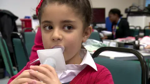
BBC Young child with brown hair, blowing air into plastic measuring device. She wears a red ribbon and red cardigan and a white shirt, She is in school, sitting on a green chair.

BBC

Children had lung function tests every year

Scientists say they have been "stunned" by how quickly young children's lungs began to recover and grow after pollution restrictions were brought in where they lived.

Researchers found that children in London whose lung growth had been stunted by pollution showed impressive improvements after the introduction of an Ultra Low Emission Zone (Ulez) in 2019 reduced emissions.

The study followed more than 3,400 primary school children in London and Luton and provides what scientists believe is the strongest evidence yet that local clean air zones could help reduce some of the harm caused by pollution during childhood.

But independent researchers caution that other factors must also be considered.

Air pollution can stunt the growth of young children's lungs leaving them at an increased risk of asthma, heart disease, diabetes and even premature death.

Children are also more vulnerable to pollution because their lungs and immune systems are still developing. And when outside, they tend to be closer to the ground and nearer sources of exhaust fumes, for example.

In 2020 Ella Adoo-Kissi-Debrah, a nine-year-old girl from London who died following an asthma attack in 2013, became the first person in the UK to have air pollution listed as a cause of death.

In the study, researchers recruited six to nine-year-olds attending primary schools in London's ultra low emission zone and followed the same children for five years, comparing them to similar children (in terms of socio-economic background, physical activity and ethnicity) in Luton.

Children in the study had annual lung function and capacity tests in the year before Ulez came in and for four years after.

Initial results showed children's lungs in London were smaller in capacity than those in Luton, which is less polluted than London but has a similar mix of pollutants.

At the end of the study the children's lung capacity reached near identical levels in both groups.

"While we would expect children's lungs to grow year on year, our results indicate that the London children's lung growth had accelerated during the four years to 'catch up' with the control group in Luton to reach similar levels of lung capacity," researchers say.

"I was absolutely stunned when I first saw the results," Prof Chris Griffiths, a senior author on the study, at Queen Mary University of London, told the BBC.

"The speed of catch up in lung capacity in the London group was surprising and impressive.

"This shows an ambitious clean air zone can drive pollution levels down, rapidly restoring children's stunted lung growth."

The main test measured how much air a child could forcibly breathe out in one second after a big breath in.

In practical terms the improvements could mean children in the London group could run as fast as the Luton group without getting out of breath or blow out the same number of candles for example, Griffiths explained.

Another way of testing for lung capacity used in the study showed significant improvements too, though not to the same extent - implying there are still gains to be made.

Overall the proportion of children in London whose lung capacity was deemed "clinically impaired" (suggesting lung damage resulting in coughs or breathlessness) fell from 14% to 9%.

In Luton - where some smaller scale measures were put in place to tackle air pollution - the figures were 9% to 7%.

The team's measurements also showed the level of nitrogen dioxide children were exposed to fell faster in London than in Luton over this time.

Researchers say this is key as it likely demonstrates that the improved lung growth they saw was related to air quality improvements following the implementation of Ulez.

London's Ulez was first introduced in 2019 by Mayor Sadiq Khan in a bid to "clean up London's air". London had high levels of the harmful gas nitrogen dioxide which comes from motor vehicles.

Older, more polluting vehicles had to pay a daily charge to drive in central London. The measures were later expanded to cover the whole capital. While many supported the policy it provoked political opposition and protests.

Prof Anna Hansell, at the University of Leicester, who was not involved in the study said the improved lung function in children was "likely to have lifelong benefits for their health."

She added the study was "carefully conducted by "well-respected researchers" and that the geographical comparisons between London and Luton were important as there had been general reductions in air pollution over time.

"This proved particularly useful, given that the study period included the Covid-19 pandemic – and demonstrates the findings in London are not due to changes related to the pandemic," she said.

Another aspect to consider was that the London group may have been more likely to walk or cycle to school once Ulez came in.

Meanwhile, Kevin McConway, emeritus professor at the Open University, said it was important to take the full impact of Covid into account and argued that studying other cities could help tease out whether some improvements were due to unmeasured differences between London and Luton.

Lead author, Dr Helen Wood, at Queen Mary University of London said while the results were very promising there was no room for complacency as "air pollution in both London and Luton – as well as other cities across the UK – remains above WHO guideline levels, so there is still work to be done".

"We know clean air zones are a complex area and the impact on businesses and individuals must be considered. What we are doing is adding new evidence to inform the debate," Griffiths said.

"There are more than a billion kids living in cities around the world, most of them in polluted environments, getting a really bad start in life.

"That's why these are important findings with global relevance."

The work involved researchers from the Universities of Bedfordshire, Oxford, Cambridge, Edinburgh and Southern California and is published in the Lancet Public Health.

The Daily Front Page 8 of 30
Wednesday, August 19, 2026 The Daily Front No. #260819 — The Inflation Ledger
article

Sticky wage norms and the real wage cost of unexpected inflation

by jplusequalt·▲ 384 points·270 comments·bfi.uchicago.edu ↗
Nominal wages did not keep pace with prices for a large share of workers who stayed at their firms.

Abstract

We use a sample of administrative payroll data covering a large and nationally representative share of U.S. workers to study how wages adjusted during the recent inflation period. Most firms apply a single modal annual nominal wage increase to the majority of their workers, and these firm-level norms changed little during the recent period of unexpected inflation. As a result, nominal wages did not keep pace with prices for a large share of workers who stayed at their firms. Forty-three percent of workers continuously employed at the same firm over the four years spanning 2021–2024 experienced a real wage decline, with a mean loss of roughly nine percent among those who fell behind. Workers could escape sticky wage norms by changing employers — job-changers’ wages rose nearly one-for-one with inflation — but switching was too infrequent to matter for most. Even accounting for job-changers, 37 percent of all workers saw real wages decline over the 4-year period. Indexing firms’ modal raises one-for-one to inflation would have closed roughly 40 percent of the resulting shortfall relative to pre-pandemic trend. Drawing on cross-country evidence from Belgium, whose wages are automatically indexed to inflation, we show that incomplete wage indexation, rather than inflation itself, helps explain the persistence of depressed consumer sentiment during the 2021–2024 period.

1 Introduction

After nearly four decades of low and stable inflation, U.S. consumer prices rose sharply and unexpectedly from mid-2021 through late-2023, with the inflation rate peaking at 9 percent in June of 2022. During this period, U.S. consumer sentiment fell to levels not seen since the depths of the Great Recession despite the unemployment rate being at historically low levels. Over 70 percent of Americans in 2022 reported that inflation was a “very big problem” (Pew Research Center 2022). In early 2024, when the inflation rate returned to normal levels, over 40 percent of Americans still claimed that “inflation/high cost of living” was the most important financial problem facing their family (Gallup 2024). Americans’ unhappiness with inflation has been cited as an important factor in voting patterns during the 2024 presidential election (Steinberg et al. 2025; Riãno and Trebbi 2026; Leonhardt 2024). Importantly, even three years after the inflation rate peaked, Americans are still reporting that inflation and affordability are pressing concerns. As of 2025, U.S. consumer sentiment remains depressed, roughly 30 percent of Americans still report that cost of living is their most pressing financial problem, and over 60 percent of Americans still report that inflation is a very big problem.

In this paper, we argue that Americans’ enduring discontent with inflation reflects the lasting real wage losses generated during the inflationary episode. Using a sample of administrative payroll data from ADP covering roughly 16 million workers per month, we examine real wage dynamics and firm wage-setting from 2016 through 2025. We show that most firms anchor annual raises to a common wage norm applied broadly across workers, and that these norms adjusted only modestly when inflation surged. Larger off-cycle raises and job changes allowed some workers to keep pace, but these responses were too limited to restore real wages for the typical worker. A temporary inflation shock therefore produced a persistent downward shift in real wages, helping explain why Americans’ dissatisfaction outlasted the inflation episode itself.

Figure 1 serves as the launching point for our paper. The figure shows a real wage index for the United States computed using either data from ADP (solid line) or data from the Current Population Survey (CPS) (dashed line). The two lines track each other closely, highlighting that the ADP data is representative of the U.S. labor market with respect to wage dynamics — a point we discuss in greater depth in Section 2.3. Median real wages fell by 4 percent during the inflation period, and did not recover to their 2020 level until late 2024. Moreover, zero real wage growth is not an appropriate benchmark for assessing whether real wages kept up. The ADP and CPS wage indices are defined by using the wage growth of a given worker over time. There is a large literature documenting that the wages of a given worker increase year-over-year due to the accumulation of general or firm-specific human capital; such life cycle wage growth occurs even in a world where there is no aggregate productivity growth. The red dashed line in Figure 1 is the predicted real wage path over the 2020–2025 period, based on extrapolating the 2017–2019 trend in the ADP data forward.

During the 2017–2019 pre-period, real wages grew at roughly 2.2 percent per year. This is in line with estimates of the annual return to experience. As of December 2025, the real wage index stands roughly 7 percent below where real wages would have been had the 2017–2019 trend continued. The 2017–2019 trend is a demanding benchmark, since real wage growth in the late 2010s was unusually strong. Measured against average real wage growth of 1.5 percent per year over the longer 2000–2019 period, the shortfall as of December 2025 was still roughly 4 percent.

The goal of this paper is to use the richness of the ADP data to shed light on the mechanisms driving the dynamics of real wages during this period. First, we document that job-stayers’ wages did not keep pace with inflation. Median year-over-year real wage growth fell from roughly 1 percent in 2017–2019 to about negative 4 percent during the inflation surge. Although real wage growth returned to its pre-period rate by mid-2023, the earlier losses were never made up, leaving job-stayers’ real wages persistently below trend.

The long panel reveals how widespread these cumulative losses were. Among workers continuously employed at the same firm from December 2020 through December 2024, 43 percent ended the period with lower real wages than at its outset; conditional on a decline, the mean loss was 9 percent and the median loss was roughly 7 percent. More broadly, 55 percent averaged less than 1 percent annual real wage growth over this 4-year period. Both the incidence and magnitude of these losses were far greater than among comparable four-year job-stayers before the pandemic. Thus, nominal wage growth failed to keep pace with inflation for a substantial share of workers who remained with the same employer.

We next examine the firm-level wage-setting practices behind these losses. Because ADP records base-wage changes for every worker within a firm, we can identify the firm-specific month in which most annual raises occur—the firm’s “on-cycle” month—and distinguish these raises from “off-cycle” adjustments in other months. Off-cycle raises are systematically larger and are consistent with worker-specific events such as promotions or responses to outside offers.

Among workers who receive exactly one wage adjustment in a year, raises cluster tightly around a firm-specific mode. A majority of all annual wage changes are within 0.5 percentage points of the modal increase, and more than 90 percent are within 1.5 percentage points. We refer to this modal increase as the firm’s “wage growth norm.” For example, during the 2017–2019 period, the modal firm had a wage growth norm of 3%, meaning that most workers received a nominal wage increase of about 3% during their on-cycle month. Critically, the distribution of wage growth norms across firms shifted only modestly during the 2021–2023 period relative to the pre-pandemic period. Roughly 89 percent of workers were employed in firms that had a wage growth norm of 2, 3, or 4 percent before the pandemic; during the inflation period, that fraction was approximately 76 percent, with a modest shift away from the 2–3 percent range toward 4–5 percent. Even as inflation rose well above prevailing wage norms, firms adjusted those norms only weakly. Because most workers’ raises were anchored to their firm’s norm, this limited adjustment helps explain the erosion of job-stayers’ real wages. Critically, these norms had been set for an era of low and stable inflation; because the inflation was unexpected, neither the norm nor workers’ initial wage bargains had priced it in, so the surprise translated directly into an unanticipated real wage loss. The stickiness we document is therefore a property of a wage-setting regime adapted to low and stable inflation, not a structural constant. Had high inflation persisted, we expect firms would have re-indexed their norms, much as cost-of-living clauses spread through U.S. collective bargaining agreements during the high inflation period of the 1970s and early 1980s.

Firms did, however, adjust on a different margin – they became more likely to grant large, worker-specific raises outside the standard annual review cycle. As a result, the within-firm distribution of nominal wage growth became more right-skewed during the inflation period. Large raises rarely arrive through the on-cycle review: on-cycle increases cluster tightly between 2 and 4 percent, while two-thirds of off-cycle increases exceed 4 percent and one-third exceed 8 percent. More notably, the share of job-stayers receiving more than one base-wage adjustment within a year rose from roughly 16–18 percent before the pandemic to approximately 27 percent in 2021 and 2022. These additional, off-cycle increases were substantially larger and more dispersed than standard on-cycle raises. Thus, rather than broadly resetting their wage norms in response to inflation, firms granted large, individualized adjustments to a growing minority of workers.

Changing employers offered workers a second way to escape sticky firm wage norms. Job-changers’ annual nominal wage growth tracked inflation nearly one-for-one, allowing them largely to avoid real-wage erosion in the year they moved. However, switching rose only modestly during the inflation period, and for any given worker, moves across employers are infrequent. This pattern means that in most years, even those who switched jobs at some point were again subject to sticky firm wage norms. Consequently, including job-changers reduces the share with a cumulative real wage decline only from 43 percent among job-stayers to 37 percent among all workers. The median loss among those who fell behind was approximately 9 percent, and 58 percent of all workers ended the period below the pre-pandemic trend.

How much of the aggregate real wage shortfall does the norm itself account for? We answer this with an accounting exercise that indexes firms’ modal raises one-for-one to inflation, holding everything else — off-cycle raises, job-changer wage growth, and the shares of workers in each group — at its observed value. Indexing that single rule closes roughly 40 percent of the gap relative to the 2017–2019 trend and roughly 73 percent of the gap relative to the more conservative 2000–2019 trend. Extending the same rule to all job-stayer wage growth closes more than half of the gap to the 2017–2019 trend and essentially eliminates the gap to the 2000–2019 trend. Together, these exercises show that a broadly applied feature of firm wage-setting, namely the weak indexation of job-stayers’ raises, can generate a large aggregate shortfall.

One implication of these firm-level patterns is that exposure to real-wage erosion should vary with workers’ access to both job switching and large worker-specific raises (e.g. promotions). We examine the implication of this for inequality across two dimensions of observable worker heterogeneity – initial wage and age.

Along the wage distribution, greater mobility initially protected lower-wage workers. The U.S. wage distribution was already compressing during 2016–2019, with workers in the bottom two deciles experiencing substantially faster wage growth than higher-wage workers. This compression accelerated in 2021: real wage growth in the bottom two deciles remained positive and close to its pre-period pace, while all other deciles experienced declines of about 2 percent, roughly four percentage points below their pre-period growth. Higher job-switching rates among lower-wage workers helped them escape sticky firm wage norms. This early acceleration in compression did not persist, however. Over the full 2021–2024 period, cumulative wage compression was similar to the pre-period: lower-wage workers continued to experience faster real wage growth relative to higher wage workers.

We also show that the real wage declines were larger for older workers. Roughly 55 percent of workers age 50 and older experienced a cumulative real wage decline between December 2020 and December 2024. Older workers had less access to both escape margins: they switched employers less often, gained less when they did switch, and were less likely to receive large raises while remaining at the same firm. Even before the inflation episode, their flatter age-earnings profiles left a larger share receiving no nominal wage increase. The inflation surge therefore produced especially large real wage losses for older workers, who have fewer opportunities to advance either within or across firms.

In the last part of the paper we provide several pieces of evidence that speak to the broader consequences of the minimal wage indexation at U.S. firms during the recent inflation period and the resulting declines in real wages experienced by U.S. workers. The real wage declines documented above are costly to the workers who experience them, but even workers who take action to overcome sticky wage norms incur costs of their own — searching for a new job, negotiating with an employer, and so on. These two types of cost are economically distinct: the effort workers expend to escape the firm’s norm is a deadweight loss, whereas the real wage decline borne by those who do not take actions is a transfer from workers to firms that benefit from the lower labor costs. We present two additional pieces of evidence consistent with this view that minimal wage indexation is costly to workers but advantageous to firms.

First, we show that the real wage growth that workers did not receive reappears, in roughly the magnitude one would expect, as higher firm profits. Between the pre-pandemic and inflationary periods, the U.S. corporate profit share of GDP rose by 1.7 percentage points — broadly consistent with the magnitude implied by the real wage shortfall we document, and its highest sustained level in half a century. The firm profit rate jumped when the inflation started in mid 2021 and remained elevated through 2025 as real wages remained depressed.

Second, we use cross-country variation to show that the lack of wage indexation, rather than inflation itself, was an important driver of the persistent decline in consumer sentiment between 2021 and 2024. Belgium offers a natural experiment: its wages are automatically indexed to inflation, insulating workers from real wage erosion, yet it experienced the same inflation, labor market conditions, and aggregate shocks — including Ukrainian immigration — as Germany, the Netherlands, Denmark, and the broader Eurozone. Real wage and consumer confidence measures diverged sharply across the countries. In Belgium, real wages rebounded to pre-inflation levels by 2023 and consumer sentiment recovered with them. In the peer countries, where wages adjusted slowly and incompletely, neither real wages nor consumer confidence had recovered by the end of 2024. We find consistent patterns within the United States across age groups. Retired households have a substantially larger share of their income indexed to inflation — through Social Security, which is indexed by law, and through asset income that kept pace with prices — whereas older workers who have not yet retired are exposed to the same sticky wage norms as everyone else. Consistent with real wage erosion driving sentiment, the decline in consumer confidence was far smaller for age groups in which most individuals are retired than for those in which few are.

Taken together, the cross-country and cross-age evidence suggests that consumer sentiment recovered when real incomes were protected, not simply when inflation subsided. In the United States, sticky firm wage norms left many workers’ real wages below their pre-pandemic trajectory, helping to explain why sentiment remained depressed through 2024.

The remainder of the paper proceeds as follows. Section 2 describes the data and assesses the representativeness of the ADP sample. Section 3 documents real wage losses among job-stayers and the firm wage-setting norms behind them, while Section 4 incorporates job-changers to characterize wage growth for the workforce as a whole. Section 5 examines heterogeneity across workers, and Section 6 quantifies the contribution of incomplete indexation to the aggregate real wage shortfall. Section 7 examines the broader consequences of incomplete wage indexation, showing that the associated real wage shortfall is quantitatively consistent with the rise in the corporate profit share and helps explain the persistent decline in consumer sentiment. Section 8 concludes.

Related Literature

This paper contributes to a large literature documenting why workers dislike inflation. Di Tella et al. (2001) show that higher inflation reduces reported life satisfaction with effects comparable in magnitude to rising unemployment, while Shiller (1997) and Stantcheva (2024) use survey evidence to document that workers link inflation directly to declining real purchasing power and reduced economic security. An alternative explanation for why workers dislike inflation is “money illusion” — the tendency to reason in nominal rather than real terms. Shafir et al. (1997) show that individuals systematically reason in nominal terms even when real quantities are what matter for welfare, and Fehr and Tyran (2001) provide experimental evidence that money illusion affects economic behavior in ways that are difficult to rationalize under standard assumptions. Our paper provides direct microeconomic evidence that distinguishes between these two stories: we show that real wages did in fact decline substantially and persistently during the 2021–2023 inflation episode, lending empirical support to the view that workers’ dislike of inflation reflects genuine real wage erosion rather than a cognitive bias. Our Belgium case-study reinforces this conclusion.

Two papers motivate our empirical analysis and provide structural interpretations for our main findings. Guerreiro et al. (2026) develop a model in which workers must take costly “conflict” actions — renegotiating their contracts, threatening to quit, or pursuing outside offers — in order to obtain nominal wage increases that keep pace with inflation. Because these conflict actions are costly, the welfare losses from inflation exceed those implied by the decline in real wages alone; workers bear an additional burden from the effort required to defend their purchasing power. This framework provides a natural interpretation for our finding that off-cycle wage adjustments rose sharply during the inflation period: workers who received large off-cycle increases had, in many cases, taken precisely the kinds of costly actions described in Guerreiro et al. (2026). For the majority of job-stayers who did not receive off-cycle raises, the cost was paid instead through passive real wage erosion. Afrouzi et al. (2026) develop a complementary model in which nominal wage stickiness induces workers with eroded real wages to search more intensively for new jobs, generating a tight link between inflation and job vacancy creation and predicting that job-changers keep pace with inflation while job-stayers accumulate losses — exactly what we document in the ADP data. Their model also allows job-stayers to pay a menu cost to escape a firm’s sticky wage growth norms thereby also reconciling the large increase in off-cycle wage increases during the inflationary period found in the ADP data. Together, both papers imply that keeping up with inflation during this episode was costly, whether through job search, conflict, or passive real wage loss. Both frameworks also share a complementary implication for firms: to the extent that adjustment costs allow employers to maintain minimally indexed wage norms, it confers a degree of market power that should be visible in firm profitability during the inflationary episode — a prediction we examine directly in Section 7.1.

A growing literature documents the political consequences of these real wage declines. Steinberg et al. (2025) use a pre-election survey experiment and find that priming voters with information about inflation reduced approval of the Biden-Harris administration, with effects concentrated among Independents and Democrats. Riãno and Trebbi (2026) use county-level variation in local prices and wages and find that it is real wage decline, not higher inflation per se, that predicts Republican electoral gains — directly reinforcing our central argument that material purchasing power losses, rather than rising prices in the abstract, drive individual discontent during inflationary periods. Baccini and Weymouth (2025) document analogous patterns in the 2022 midterms, suggesting these links between real purchasing power and electoral behavior are not unique to the 2024 presidential cycle. Using micro data for large and representative sample of the U.S. workforce, we document that the wages of a large share of Americans did, in fact, substantially decline from early-2021 through late-2024 explaining their overall discontent with their economic situation expressed via their voting behavior.

Finally, our documentation of firm-level wage-setting norms connects to a long literature on nominal wage rigidity and fairness. Bewley (1999) concludes from interviews with managers that firms resist nominal wage cuts primarily to protect worker morale, while Akerlof and Yellen (1990) and Kahneman et al. (1986) formalize the role of fairness norms in wage-setting and show that workers withdraw effort — and firms restrain exploitation of demand shocks — when perceived fairness is violated. These papers establish that nominal wage rigidity reflects social norms rather than purely technological constraints, which is exactly the kind of norm our ADP data reveals at the firm level. Hazell and Taska (2025) provide complementary evidence using posted vacancy data that wages for new hires are asymmetrically rigid — downwardly sticky but responsive to labor market tightening — suggesting that the structural features underlying our findings are broad. Grigsby et al. (2021b) and Grigsby et al. (2021a) use the ADP payroll data during prior periods showing, among other things, that nominal wages of job-stayers are downwardly rigid. All of this prior literature focuses on various aspects of downward nominal wage rigidity. Our paper shows a similar pattern with wage norms for job-stayers being upwardly rigid during periods of rising temporary inflation.

2 Data Description

In this section, we describe the data used in the paper and provide some motivating descriptive statistics using the data.

2.1 ADP Data

The majority of our analysis uses administrative individual panel data from ADP. ADP is a large, international provider of human resources services including payroll processing, benefits management, tax services, and compliance. ADP has over 1 million clients worldwide, and currently processes the payroll for one-sixth of the U.S. labor force. Our starting analysis sample contains the payrolls for roughly 16 million U.S. workers per month. Our sample includes firms with 50 or more employees to capture wage setting norms within and across employers. We restrict our analysis to payroll observations between December 2015 and December 2025.

Firms contract with ADP to process the payroll for all workers within their firm. As a result, we observe how nominal wages are adjusted for all workers within a given firm during a given month. This feature of the data allows us to examine the similarity of nominal wage changes across workers within a firm during a given time period. Our sample dataset includes roughly 60,000 unique firms each month.

The data contain monthly aggregates of anonymized individual paycheck information, as well as all relevant information needed for human resources management. Crucially, we observe the statutory per-period before-tax contract rate for all employees. We refer to this as a worker’s “base” hourly wage. For workers paid hourly, the worker’s base wage is simply their contracted hourly wage at the firm. For salaried workers, their base wage constitutes the pay that the worker is contractually obligated to receive each pay period (weekly, bi-weekly, or monthly) expressed in units of an hourly wage assuming a 40 hour work week. Given the data are aggregated to the monthly level, the base wage is measured as of the last pay period of the month.

In addition to the administrative base wage information, the ADP data contain all other information that would appear on the worker’s paycheck, such as the worker’s gross earnings per pay period and any bonuses that were paid to them by the firm. The data also contain other payroll information including whether the worker is paid hourly, the frequency at which the worker is paid and the number of hours paid during the month for hourly workers. We also observe various additional geographic and demographic characteristics of a worker such as gender, age and worker tenure as well as details about the job such as firm size, and industry.

We separately examine nominal wage adjustments for “job-stayers” and “job-changers”. Our primary job-stayer analysis examines year-over-year nominal base wage changes for a given worker who remains employed at the firm continuously for 13 consecutive months. For example, to measure the change in nominal base wages for a job-staying worker between March 2022 and March 2023 the worker would have to be continuously employed at the firm for all months between March 2022 and March 2023. We have between 9 and 11 million job-stayers per month in all months of our analysis during our sample period. Our primary job-changer analysis examines year-over-year nominal wage adjustments for a given worker currently working at firm i in month t who we can find working at a separate ADP firm j in month t − 12 (one year earlier). The ADP data is so large that we have about 1 to 2 million job-changers each month. In some of our analysis, we will define job-stayers and job-changers over four or five-year periods.

2.2 CPS Data

We benchmark the wage dynamics of workers within our ADP sample to the wage dynamics of workers within the Current Population Survey (CPS) as reported by the Atlanta Fed’s Wage Tracker Index. CPS respondents are surveyed for four consecutive months (waves 1-4), leave the survey for the next 8 months, and then are surveyed again for another four consecutive months (waves 5-8). In waves 4 and 8, which are one year apart, CPS respondents are asked about their hourly wage (if they are hourly workers), their usual weekly earnings and their usual weekly hours worked. This data allows the creation of a worker’s base wage in those two waves where the base wage of workers paid hourly is their reported hourly wage; the base wage of salaried workers is usual weekly earnings divided by usual weekly hours.

The Atlanta Fed uses the CPS data to create a measure of a given worker’s annualized base wage growth by taking the percentage change in base wages between waves 4 and 8. Pooling across all workers in wave 8 during each month, they then report the median nominal wage growth for U.S. workers at the monthly level.

We download the CPS wage data directly from the Federal Reserve Bank of Atlanta’s Wage Growth Tracker website. We use their monthly measure of “overall median nominal wage growth weighted using 1997 weights” when making our CPS wage indices. To make the aggregate CPS real wage index, we first make a nominal wage index using the reported nominal wage growth rates for each month. We normalize the nominal wage index to a value of 1 in January of 2017. We then deflate the nominal wage index into real January 2017 prices by appropriately deflating by the corresponding monthly CPI-U. This is how the dashed line in Figure 1 was created.

2.3 Representativeness of the ADP Data

The ADP data has been shown to be quite representative of the US labor market. For example, as seen from Figure 1, the real wage index computed using our ADP sample matches nearly identically the real wage index computed using CPS data as reported by the Atlanta Fed. Furthermore, as documented in Grigsby et al. (2021b) and Cajner et al. (2019), the overall ADP data is very representative of the US workforce based on demographic characteristics and labor force dynamics. Comparing to U.S. Census data, Grigsby et al. (2021b) shows that the ADP data also matches well both firm size and industry composition conditional on restricting the Census data to firms with at least 50 employees. In our baseline analysis, we do not reweight the ADP sample to match the QCEW industry-by-firm-size distribution, as doing so has virtually no effect on the results. Appendix Figure R1 shows that the aggregate real wage index in Figure 1 is nearly identical with and without reweighting. This insensitivity reflects the broad representativeness of the ADP sample and the limited systematic variation in nominal wage adjustments across industries and firm sizes. We further illustrate this point throughout the paper by discussing our results separately by industry.

2.4 Descriptive Statistics of Nominal and Real Wage Growth: ADP Sample

Panel A of Figure 2 displays the year-over-year median nominal wage growth of job-stayers and job-changers in our ADP sample. Panel B shows the corresponding year-over-year median real wage growth rates. A few things are of note from the two panels. First, the median nominal wage growth of job-stayers was exactly 3% from January 2016 through March 2021. As we show below, this results from the fact that firm wage norms are prevalent, with roughly 14% of all U.S. workers receiving a nominal wage increase of exactly 3.00 percent in most months during our sample period and 21% receiving an increase between 2.9 and 3.1 percent. Second, the median nominal wage growth of U.S. job-stayers did not keep up with inflation during the inflation period. During the 2017-2019 pre-period, the median real wage of job-stayers was increasing by about 1% per year. However, between all months between early-2021 and early-2023, median real wage growth was negative for job-stayers. During early-2022, the median real wage of job-stayers contracted by roughly 4%. Third, there was no rebound in the median real wage growth of job-stayers when the inflation period ended. From mid-2023 through late-2025, the median real wage growth of job-stayers was roughly back to pre-period levels of roughly 1% per year. Finally, the median nominal wage growth of job-changers increased sharply during the inflationary period. As seen from the dashed line in panel B, median real wage growth of job-changers increased by about 4% per year during the inflationary period. As we discuss below, the wage growth of job-changers did not systematically deteriorate during the inflationary period.

The above data are used to make the ADP real wage index shown in Figure 1. In particular, we pool together the nominal wage growth of job-stayers with the nominal wage growth of job-changers in each month to create an aggregate median nominal growth rate. Using the ADP data, we can compute the share of ADP employees in month t − 12 who remain continuously employed at the same firm through month t and the share who are working at another ADP firm in month t. Adjusting the job-changing share for the fact that our sample of ADP firms comprise approximately one-seventh of U.S. employment, we create a series of the relative weights of job-changers and job-stayers to construct a pooled nominal wage growth rate. We make a nominal wage index using the aggregate growth rates where we normalize the index to 1 in January 2017. We then deflate the nominal wage index by the corresponding monthly CPI, with January 2017 as the base year, to create the aggregate real wage index shown in Figure 1.

While the ADP and CPS real wage measures track each other closely, it is important to highlight a key limitation when using the CPS data to separately measure the wage growth of job stayers versus job changers. The CPS does not contain information on whether an individual switches to another firm between waves 4 and 8 and, as a result, job-changing status must be imputed. The CPS data processed by the Atlanta Fed imputes whether the individual changed jobs based upon whether the individual reports that either their occupation or industry changed between the 9 months spanning waves 4 and 6. This induces two types of measurement error. First, some job-changers will be included in the job-stayer sample if they changed firms but remained in the same occupation or industry. Second, some job-stayers will be included in the job-changer sample if their occupation or industry was misreported. It has been found that there is a large amount of measurement error in the CPS occupation and industry codes (e.g., Kambourov and Manovskii (2013)).

These two types of measurement error will narrow the gap in the wage change between job-stayers and job-changers. Panels A and B of Figure 3 show the median nominal wage growth of job-stayers and job-changers, respectively, in the CPS data (dashed line). For comparison, we also re-display the ADP nominal wage growth of job-stayers and job-changers (solid line). Consistent with the direction of the measurement error, the median nominal wage growth of job-stayers is slightly higher in the CPS data while the median nominal wage growth of job-changers is substantially lower in the CPS data. The gap in nominal wage growth for job-changers between the ADP and CPS data is particularly striking during the 2021–2023 inflation episode, when ADP records median nominal wage growth for job-changers exceeding 12 percent while the CPS measure peaks at about 8 percent. These results suggest that researchers should proceed with caution when examining wage dynamics separately for job-changers and job-stayers using the CPS data.

3 Wage Growth Within Firms

There are two notable features of the nominal and real wage dynamics of job-stayers shown in Figure 2 that motivate the analysis in this section. First, median real wages of job-stayers fell sharply during the inflation period, even as their median nominal wages rose; nominal wage growth was positive but simply not enough to keep pace with inflation. Second, the median nominal wage growth of job-stayers was exactly three percent in every month from January 2017 through early 2020. A persistent exact three percent median nominal wage growth is difficult to reconcile with a model in which firms continuously reoptimize wages worker-by-worker in response to changing market conditions. It points instead to something more institutional: many firms maintain a modal annual raise of exactly 3% that applies broadly and uniformly to a large share of their continuing workers.

In this section, we look inside the median to characterize the full distribution of real wage changes for job-stayers, document the firm-level wage norms that generate that distribution, and show that those norms adjusted only modestly during the inflation surge. We also show that an increasing number of workers escaped their firm’s wage norm during the inflationary period by receiving multiple wage adjustments within a year — a pattern consistent with workers taking costly actions to negotiate for higher pay. The result, for job-stayers, was a distribution of nominal wages that shifted up with inflation, but also a distribution of real wages that shifted meaningfully down.

3.1 The Distribution of Annual Nominal Wage Growth, Job-Stayers

Figure 4 reports the distribution of annual nominal base-wage changes for job stayers, defined as those workers continuously employed at the same firm for at least thirteen consecutive months. Panel (a) compares the pre-pandemic period (2016–2019) with the high-inflation period of 2021–2023. Panel (b) repeats this comparison but showing the recent period of 2024–2025 against the same pre-pandemic baseline. Several features of these distributions are worth noting.

In the pre-pandemic period, the distribution is concentrated in the range of two to four percent annual nominal growth. Approximately 21.9% of job stayers received no nominal wage change over the preceding year. Conditional on a nominal wage increase, the modal change was between 2 and 3 percent, with 51.4% receiving between 1 and 4 percent, 26.0% between 4 and 10 percent, and 5.6% more than 20 percent. The figure is truncated at zero because nominal wage cuts were exceedingly rare, with only 1.7% of workers in this period getting nominal wage cuts. These patterns are broadly consistent with earlier findings using ADP data from the 2008–2016 period reported by Grigsby et al. (2021b). The somewhat lower incidence of zero nominal wage growth in our pre-pandemic sample, relative to their earlier period, likely reflects the stronger labor market conditions that prevailed between 2016 and 2019.

During the high-inflation period of 2021–2023, shown in Panel A, the distribution of nominal wage growth shifted to the right. The share of job stayers with no nominal wage change only fell minimally to 19.1%. The largest shifts occurred in the interior of the distribution. Conditional on receiving any nominal wage increase, the median increase rose to between three and four percent. Additionally, conditional on receiving a raise, the share receiving an increase between 1 and 4 percent fell to 35.1% while shares receiving an increase between 4 and 10 percent and above 20 percent rose to 34.0% and 8.7%, respectively. Workers receiving increases above 20% likely include those who received promotions or experienced other substantive changes in their roles. Despite the rightward shift in the distribution, more than half of job-stayers had annual nominal wage growth below 4% even as year-over-year inflation rose above 7%.

After the inflation period, the nominal wage growth distribution for job-stayers mostly returned to the pre-period baseline. The 2024–2025 distribution is shown in Panel B. The fraction of workers with the large pay increases generally associated with promotions returned to pre-pandemic level of around 5.0%, and the distribution largely resembles its pre-pandemic counterpart, with the exception that the modal wage change shifted up slightly. In 2024–2025, workers were getting more wage increases between 3-5% and fewer increases between 1-3%. During this period, both the annual inflation rate and the average nominal wage growth increased by about one percentage point relative to the pre-pandemic period.

3.2 The Distribution of Cumulative Real Wage Growth, Job-Stayers

While Figure 4 shows that the distribution of nominal wages clearly shifted upward during the recent inflationary period, workers care about their real wages, which are governed by the relative movement of inflation and nominal wages. As we saw in Figure 2, real wages of the median worker fell sharply during the inflationary period. Moreover, looking only at the distribution of annual wage changes leaves open the possibility that workers who received relatively small increases in one year may have been compensated with larger increases in subsequent years, so that the cumulative experience of a long-tenured job stayer may have been more or less favorable than these annual snapshots suggest.

To trace how these cumulative losses accumulated as the inflationary period progressed, Table 1 reports the share of job-stayers experiencing a real wage decline over progressively longer horizons — one, two, three, and four years — beginning in December 2020, alongside the analogous pre-period statistics beginning in December 2015. We then turn to the full distribution of four-year changes in Figure 5. When computing the cumulative real wage changes over multiple years we restrict our sample to workers who were continuously employed at the same firm over the corresponding time period. For example, for the two-year wage change, workers must have remained continuously employed at the same firm between December 2020 and December 2022. We compute real wage changes by deflating the worker’s nominal wage in a given month by the corresponding CPI in that month.

Dec 2020 Job-Stayers: Share w/ Real Wage Decline Conditional Mean Real Wage Decline Share Job-Stayers Dec 2015 Job-Stayers: Share w/ Real Wage Decline Conditional Mean Real Wage Decline Share Job-Stayers
One-Year 66.5% −5.1% 67.4% 37.7% −2.2% 74.2%
Two-Year 57.4% −7.7% 48.3% 29.2% −3.9% 55.4%
Three-Year 49.3% −8.3% 36.9% 24.4% −5.3% 41.9%
Four-Year 43.0% −8.9% 29.1% 21.4% −6.9% 31.9%

The first three columns of Table 1 summarize the share of job-stayers with a real wage decline over horizons beginning in December 2020; the last three columns report the analogous pre-period statistics beginning in December 2015. As shown in the top row, two-thirds of job-stayers experienced a real wage decline during 2021, averaging roughly 5 percent among those who fell behind. The U.S. experienced a 7 percent inflation rate during 2021, but, as we show later, the median worker during this period received a nominal wage increase of only about 3 percent. These losses were large relative to a lower-inflation period. For comparison, during the pre-period, a little over one-third of workers experienced a real wage decline, with the mean decline for these workers being a modest 2.2 percent.

The fact that real wages fell during 2021 when inflation was high is not surprising. Most sticky-wage models predict real wage declines during a year of inflation, given that nominal wages adjust with a lag. What is more surprising is how persistent these losses were: half of continuously employed workers still had lower real wages three years later, and 43 percent remained below their starting real wage four years later. Moreover, as the horizon lengthens, the share of stayers with a real wage decline falls from two-thirds at one year to 43 percent at four, but the mean decline among those who fall behind grows from roughly 5 percent to nearly 9 percent. Some workers were able to escape declining real wage growth as time progressed, but a substantial minority have nominal wages that persistently failed to keep up with the burst of inflation.

We now turn to the full distribution of four-year changes underlying the last row of Table 1, shown in Figure 5. Panel (a) reports the probability density functions of the four-year real wage changes of job-stayers during the inflation period and the pre-period, while Panel (b) reports the corresponding cumulative distribution functions. In the pre-period, real wage growth for the median worker was between 4 and 6 percent over the four-year period spanning 2016–2019. Twenty-one percent of workers experienced negative real wage growth during this period, with almost 5 percent seeing real wages fall by around 8 percent as a result of receiving zero nominal wage growth in every period, given the inflation rate averaged about 2 percent per year. Among those with negative real wage growth, the median decline in real wages was around 4 percentage points. For those who saw a rise in their real wage, the median real wage growth was roughly 6 to 10 percentage points — or 1.5 to 2 percent per year.

The growth in real wages in the four-year period between 2020 and 2024 looked meaningfully different. The distribution of cumulative wage growth during the inflation period lies substantially to the left of its pre-pandemic counterpart, with the leftward shift being reasonably uniform across the distribution. During this period, the median worker saw real wage growth of only between 2 and 4 percent (0.5 to 1.0 percent per year).

The share of workers taking persistent real wage losses was also far larger during the inflation period. As noted in the last row of Table 1, fully 43 percent of four-year job-stayers experienced declines in their real wages. Moreover, among those with negative wage growth, the decline was large, with a mean decline of nearly 9 percentage points and a median declining of roughly 7 percentage points. In other words, over 20 percent of all workers within the United States who stayed with their employers experienced a real wage cut of roughly 7 percent during the four-year period spanning 2021–2024.

Taken together, Figures 4 and 5 and Table 1 establish a key feature of wage growth within firms during the inflationary period. For workers who remained at their firms, nominal wages rose but not nearly enough to keep up with inflation, resulting in meaningful declines in real wages for a substantial share of workers. These declines persisted through 2024.

3.3 Understanding Within-Firm Wage Growth: Strong Wage Norms

The rightward shift in the distribution of annual wage changes during 2021–2023, while notable, was far smaller than the inflation shock that drove it, leading to large declines in real wages for many job-stayers and much lower real wage growth than normal for others. The obvious question is why. We now show that the answer lies in a key institutional feature of within-firm wage setting: most firms apply a single modal annual raise to the large majority of their continuing workers, and this wage setting norm moved only modestly during the inflationary episode.

We begin by showing that even in the overall distribution of annual wage changes for job stayers, the discreteness in Figure 4 masks even sharper bunching of wage growth around round numbers. Figure 6 breaks down the distribution of annual wage changes by highlighting how many nominal wage changes occurred at exactly whole numbers (e.g., 1, 2, 3, 4, etc.), exactly half numbers (e.g., 1.5, 2.5, etc.), or any other number during the 2017-2019 pre-period. The figure shows that between 2016 and 2019, among those workers who received a wage change of between 1 and 6 percent, a full 14% had nominal wage changes of exactly 3% while 21.1% were between 2.9 and 3.1 percent. Roughly 42% of all nominal wage increases below 6% were within 0.01 percentage points of a whole or half number. This stark bunching at round numbers is difficult to reconcile with a model in which firms individually reoptimize each worker’s wage in response to that worker’s idiosyncratic productivity or outside option. It instead suggests that firms adopt simple wage-setting conventions, wherein they give many workers a uniform 2, 2.5 or 3 percent wage increase.

Figure 6 establishes that nominal wage changes cluster sharply at round numbers in the aggregate. We now assess the extent of the dispersion in nominal wage growth within a firm and how that dispersion changed during the inflation period. For each firm-year, we identify the “on-cycle” month as the month in which the largest share of workers receive a nominal wage adjustment and define the firm’s wage norm as the modal adjustment made in that month. At nearly all firms, the vast majority of annual wage adjustments occur in this single month. When computing the modal nominal wage change during the on-cycle wage adjustment month, we group nominal wage changes within the firm into one percentage point bins centered around whole numbers. We restrict our sample to those workers within the firm who experienced one nominal wage change during the calendar year. To ensure that the inferred modal change reflects a genuinely broadly applied rule rather than idiosyncratic noise, we further restrict the sample to firm-years in which at least 30 percent of workers received a positive nominal wage increase and at least 30 percent of those received the modal increase. The resulting measure captures the annual raise that a continuing worker at that firm would expect to receive absent a worker-specific adjustment.

Figure 7 shows that during a given year, most workers within a given firm receive a nominal wage increase of a similar size. Specifically, in Figure 7, we plot the distribution of nominal wage changes for all workers receiving a wage increase relative to the firm’s own wage growth norm in that year. Among workers who received a wage increase within 5.5 percentage points of the firm’s norm, almost 60 percent received a wage increase that was within half a percentage point of their firm’s mode. Again, the data reveal that firms for the most part are setting compensation growth similarly for most of their workers as opposed to individually tailoring wage growth to each worker.

Because this firm-level wage norm applies to the majority of workers, a key input to understanding the behavior of wages within the firm during the inflation period is to understand how this firm-level wage norm evolved over this period. Figure 8 reports the cross-firm distribution of these firm-level wage norms, weighting firms by their number of employees. Panel (a) compares the pre-pandemic period to the high-inflation period and Panel (b) compares the pre-pandemic period with 2024–2025. Before the pandemic, the distribution was tightly concentrated. Indeed, 56% of workers were employed at firms whose modal wage change was between 2.5 and 3.5 percent, consistent with the large bunching at precisely 3% seen in Figure 6.

During the high-inflation period, firms only marginally adjusted their wage rules. 46.5% of workers were still at firms with a wage norm of between 2.5 and 3.5%. Roughly 88.9% of workers were employed in firms that had a wage growth norm in the 2-4 percent range before the pandemic. During the inflation period, that fraction fell modestly to 76.2%, with a slight shift away from the 2–3 percent range toward 4–5 percent. At the peak of the inflation period with prices increasing by over 7% per year, most workers were employed in firms with a wage growth norm in the 2-4 percent range. By 2024–2025, the modal wage norm of around 3% growth was restored, but more firms adopted wage norms around 4% and fewer held a norm of 2%.

Figure 9 makes the point that firms did not systematically adjust their wage norms during the inflation period by looking at the evolution of these firm-level wage rules over time. The figure plots the employment-weighted average modal wage change across firms alongside inflation rate from 2016 through 2025. In the pre-pandemic period, firm-level wage rules were relatively stable at a median of 2.7%, modestly above the rate of inflation. Beginning in 2021, inflation rose sharply, peaking at approximately seven percent in 2022. The average modal wage change also rose, reaching a peak of 3.5% in 2022 and 2023. By 2025, the median firm had a wage rule granting increases of three percent, roughly in line with inflation in that year. The stickiness of firms’ wage rules in the face of inflationary pressure contributed to the systematic fall in real wages for job stayers.

3.4 Wage Adjustments Outside the Firm’s Wage Rule

The preceding results show that the median firm’s wage rule responded only modestly to inflation. However, a second margin of within-firm adjustment is the extent to which individual workers deviated from this wage norm through off-cycle wage increases. In this subsection, we examine this margin.

To begin, Figure 10 plots the fraction of job stayers who received more than one nominal base-wage change within a twelve-month period, measured annually from 2016 through 2025. In the pre-pandemic period, approximately 16 to 18 percent of workers received more than one wage change within a year. However, in 2021 and 2022, the fraction of workers receiving multiple wage changes within a year rose sharply to 27 percent. By 2023, this share had begun to decline, and by 2025 it had returned to slightly below its pre-pandemic level. The spike in the frequency of wage changes during the inflationary period indicates that firms became substantially more likely to make off-cycle wage adjustments outside the firm’s standard annual review cycle. This pattern is consistent with worker actions being increasingly important for wage growth during this period (Guerreiro et al., 2026; Afrouzi et al., 2026).

Figure 11 compares the distributions of on- and off-cycle nominal base-wage increases, pooling observations from 2016–2025. The distributions differ sharply. On-cycle increases are tightly concentrated between 2 and 4 percent, consistent with the modal raises documented above. Off-cycle increases are substantially more dispersed and skewed toward larger values: two-thirds exceed 4 percent, one-third exceed 8 percent, and almost 20 percent exceed 12 percent. These off-cycle adjustments likely reflect worker-specific events such as promotions, renegotiations, or merit increases.

Figure 12 shows how the median on-cycle and off-cycle wage changes evolved through this period. The default on-cycle norm of a 3% increase for on-cycle wage changes is again evident in the figure. For the years 2016-2020, the median on-cycle wage change was exactly 3%. Off-cycle wage changes are consistently above on-cycle changes throughout the sample period, but the gap widened considerably during 2021 and 2022, when the median off-cycle increased by around 1.5 percentage points while the median on-cycle increase rose only 1 percentage point.

3.5 Bonus Adjustments: Job Stayers

All of the above figures focus on movements in employees’ base wages. However, another margin of adjustment that firms could use to compensate workers for their minimally indexed wage rule is to adjust other forms of compensation, namely bonuses. Indeed, on average, 18 percent of workers received a bonus in December from 2017–2019, but that number rose to 22 percent from 2021–2023. However, despite the increased prevalence of bonuses during the inflationary period, they did very little to stem the real wage losses that workers experienced.

The cumulative real wage distribution for job-stayers is nearly identical with and without bonuses. This is because bonuses are generally small as a fraction of total compensation for most workers, and one-off payments are poorly suited to offset the kind of real wage erosion that accumulates continuously over a multi-year inflationary episode. For example, a bonus received in December 2022 may partially offset the real wage loss in that year, but it does nothing to restore the base wage from which all future raises are calculated. Because firms’ wage rules apply to base wages rather than total compensation, a worker who receives a bonus but no adjustment to their base wage will continue to fall behind inflation in every subsequent year, with the gap compounding over time.

3.6 Summary

Taken together, the evidence in this section points to a coherent picture of within-firm wage setting during the inflationary episode. Firms operated with strong wage rules that determined the nominal wage growth for the majority of workers, and adjusted these rules upward only modestly in response to inflation. The resulting gap between the modal wage change and inflation was the primary driver of real wage erosion among most job stayers. At the same time, firms showed considerably more flexibility in responding to individual worker circumstances, delivering substantially larger increases to workers who took actions that resulted in off-cycle wage adjustments. These off-cycle increases helped to moderate, but did not eliminate, the real wage losses experienced by workers who remained within their firms throughout the inflationary episode.

4 Overall Wage Growth: Accounting for Job-Changers

The preceding section established that within-firm wage adjustment during the inflationary episode was constrained by the stickiness of firms’ wage rules. An alternative mechanism by which workers could recover lost real wages was to change employers. Indeed, the 2021-2023 period was one in which there was a notable increase in the fraction of workers who switched employers. Specifically, during 2016-2019, an average of 2.24% of employed workers switched jobs each month, while that number rose to 2.38% per month during the 2021-2023 inflationary period (Afrouzi et al. 2026). Figure 2 also shows that the real wage growth of workers who changed firms, the “job-changers”, appeared to keep up during the inflationary period. In this section, we characterize the full distribution of wage changes for job-changers, assess how that distribution has changed during the inflation period, and compute a measure of cumulative four year wage growth for all workers in the economy combining both information on job-changers and job-stayers.

4.1 Wage Growth of Job Changers

Before showing the full distribution of wage changes for job-changers, we provide additional evidence on how the median wages of job-changers evolved relative to job-stayers as the inflation rate changed. Figure 2 above shows that nominal wage growth for job changers in any given period is higher than the nominal wage growth for job stayers, and the gap widened substantially during the inflationary period as job stayers experienced relatively modest nominal wage growth and job changers experienced large increases. Figure 13 makes this point more precisely by plotting, for each calendar month, median annual wage growth against the year-over-year inflation rate separately for job stayers and job changers. As we discussed in detail in Section 3, the nominal wages of the median job stayer in each month were very weakly indexed to inflation. This is especially true for workers subject to the firm’s wage norms, but also true even after accounting for any deviations from the firm’s wage norm that workers received. This contrasts with the median job changer, whose nominal wage growth was not only higher on average but tracked inflation nearly one-for-one. Formally, regressing median monthly wage growth on year-over-year inflation yields a pass-through of 0.96 for job-changers and just 0.27 for job-stayers. The slope of the firm’s wage norm with respect to inflation is even lower at 0.082. Therefore, in any given year, switching employers was the more reliable means of obtaining nominal wage growth that kept pace with contemporaneous inflation.

The time-series evidence on median wage growth, however, masks considerable heterogeneity in the experience of individual job changers. Figure 14 reports the distribution of annual nominal base-wage changes for these job changers, comparing the pre-pandemic period with the high-inflation period of 2021–2023 (Panel a) and the recent period of 2024–2025 (Panel b). Consistent with Grigsby et al. (2021b), in all periods, the distributions for job changers are strikingly more dispersed than those for job stayers documented in Figure 4. Both large nominal wage gains and large nominal wage losses are common among changers.

Comparing Panel (a) with the corresponding stayer distribution reveals that the inflationary episode had a qualitatively similar effect on job changers as on job stayers: both distributions shifted to the right. What differed was the magnitude. For job stayers, the rightward shift was modest, with the median increase rising by roughly one to two percentage points relative to the pre-pandemic period. For job changers, the shift was substantially larger. Among job changers, the fraction of job changers with negative wage growth dropped from 28.6% to 24.9%. The result was a widening of the already large gap in nominal wage growth between job changers and job stayers during the inflationary episode. Panel (b) shows the corresponding distribution for 2024–2025. As inflation receded, the job-changer distribution shifted back toward its pre-pandemic shape, and the gap in nominal wage growth between job changers and job stayers narrowed as well.

4.2 The Overall Effect of Recent Inflation on U.S. Real Wages

The previous section showed that the median wage gains available to job changers during the inflationary episode were substantially larger than the within-firm adjustments available to job stayers. This raises the question of whether cross-firm mobility was sufficient, in aggregate, to offset the real wage erosion documented in Section 3 for job-stayers. Figure 15 addresses this question by reporting the distribution of cumulative real base-wage growth for all workers — both job stayers and job changers combined — over the two four-year windows of December 2015 to December 2019 and December 2020 to December 2024. Panel (a) reports the probability density function and Panel (b) reports the cumulative distribution function.

Panel (b) of Figure 15 contains the central result of the paper. Even after incorporating the large wage gains available through job changing, 37.0% of U.S. workers experienced a cumulative decline in real wages over the four years from December 2020 to December 2024. This is 1.6 times larger than the 23.6% of workers who saw a real wage decline over the comparable pre-pandemic window. Moreover, this share is only slightly lower than the 42.8% of job-stayers that experienced real wage declines during the 2021-2024 period which shows that incorporating job-changers does not meaningfully alter the findings. And for those who fell behind during the 2021-2024 period, the losses were

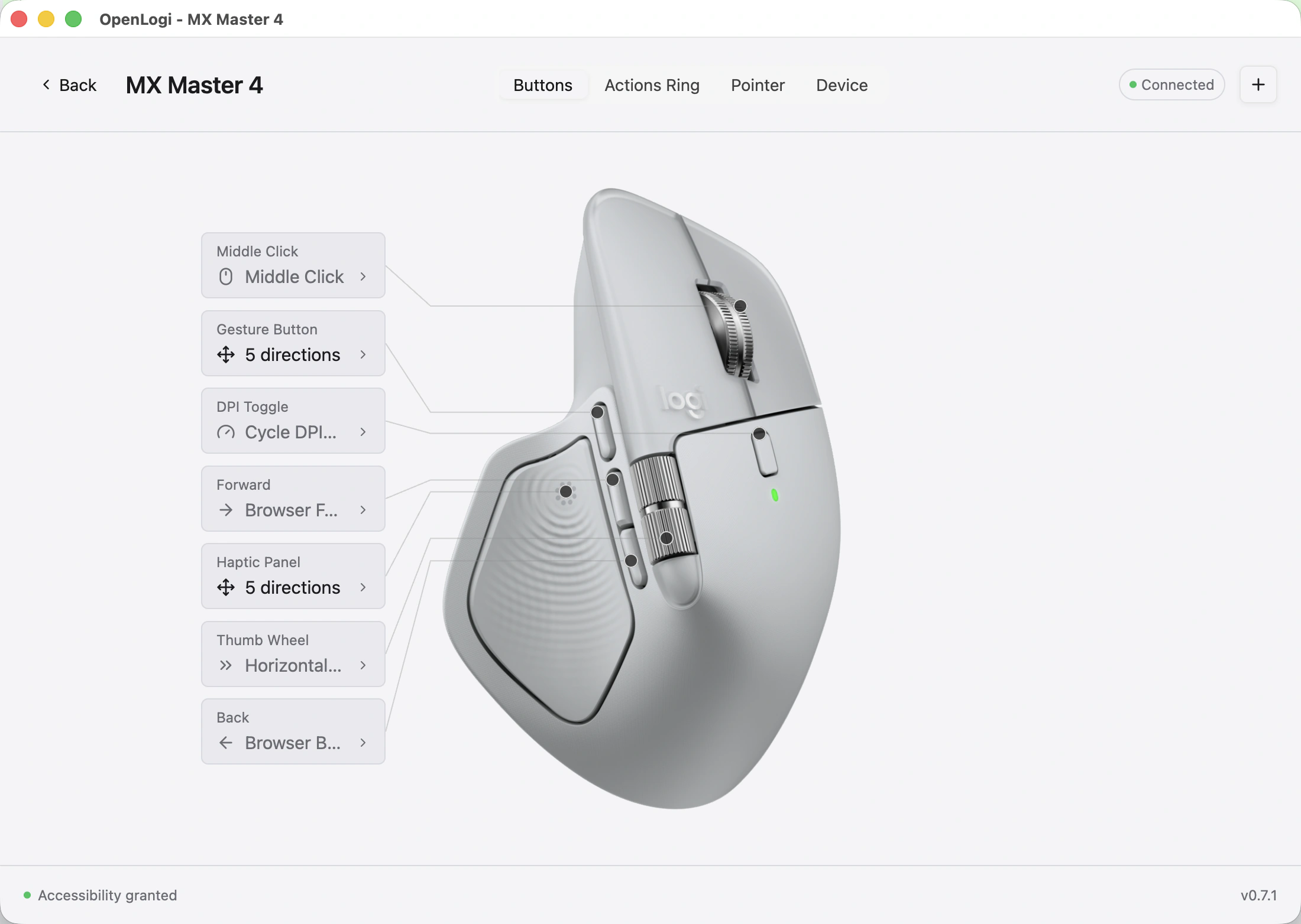
The Daily Front Page 9 of 30
Wednesday, August 19, 2026 The Daily Front No. #260819 — Postgres, Apparently
article

PostgreSQL for Everything

by karlmush·▲ 349 points·214 comments·raphaelbauer.com ↗
Contrary to popular belief - the answer to everything is NOT 42 - it’s PostgreSQL.

PostgreSQL for Everything

Contrary to popular belief - the answer to everything is NOT 42 - it’s PostgreSQL. (ok. It might also be Postgres).

Intro

I started using PostgreSQL roughly in 2003 for a research project called ColumbaDB. Columba is no more, but PostgreSQL is still alive and kicking more than ever.

In 2003, MySQL was much more widely used than PostgreSQL. MySQL was also potentially faster as it did not implement all features of the SQL standard. At the same time MySQL was lacking many features that we needed (full-text search, powerful indexes, SQL standard compliance etc). PostgreSQL felt more like a “real” database in comparison to MySQL - like a tiny version of Oracle - but in open source clothes.

During that research project I learned a lot about databases, indexes and the power of PostgreSQL. One important use-case was full-text search. We could have used MySQL in conjunction with another system like Lucene / Solr to make our database searchable. But that would have meant running and maintaining two such systems. Complicated.

PostgreSQL allowed us to use a fulltext search plugin to do everything in one system. No need to sync any data. No need to maintain and run two systems. It just worked and made us smile (after some tweaks of course). Simplicity.

Since then I used PostgreSQL for many use-cases throughout my career as CTO / Interim Manager. Most recently I used PostgreSQL to store very high volume web analytics time series data via its TimescaleDB plugin. Check out Privatracker - the best way to do web analytics and respect the privacy of your visitors - to see it in action.

Many others discussed the topic from different angles. And each article is really worth your time (SQL is Agile, Stephan Schmidt on Using SQL for Everything). Also check out my Linkedin post.

And if you are using PostgreSQL I can highly recommend reading Hazel Bachrach’s nice post on “What I Wish Someone Told Me About Postgres”.

In my humble opinion the power of PostgreSQL comes from three sources:

  1. It is rock-solid and stable.
  2. It is easy to run, install and scale.
  3. It massively simplifies your IT setup by being not only a RDBMS, but also a full-text search engine, a document storage and much much more…

Let’s have a closer look…

Rock Solid and Stable

PostgreSQL is boring old technology. The first PostgreSQL release dates back to 1996. PostgreSQL is also very widely used - for a very long amount of time. Ironing out bugs - especially in database systems - takes time. PostgreSQL had that time.

It also has a very active community that diligently adds more and more features without breaking any old parts of it. In recent years PostgreSQL got many amazing features like json document storage, partitioning support, common table expressions and much much more. Each new release of PostgreSQL is exciting and brings new nice features.

True - PostgreSQL is old - but the features are very very modern - and PostgreSQL becomes better with every release.

Easy to Run, Install and Scale

PostgreSQL can be installed very easily locally. It is bundled with all major Linux distributions, part of Mac brew, but can also be installed with applications like PostgresApp.

When running tests, it comes in handy using Testcontainers with PostgreSQL. It was never easier running your tests against a real PostgreSQL database that is 100% similar to the production thing.

If you want to run PostgreSQL on a server then you can simply apt-get install it. Or run it in a docker container.

All cloud providers allow you to run (and scale!) PostgreSQL by clicking a single button. You got ample of choice at your fingertips:

That makes PostgreSQL one of the most widely supported software systems in the market. And for you this means less maintenance and more time for creating new features for clients.

Simplifies Your IT Setup

Running PostgreSQL in the cloud is already just one click. But it gets even better. PostgreSQL can replace many systems that youd’d have to run otherwise.

PostgreSQL Replaces Solr and Elastic: Full-Text Search

PostgreSQL allows you to turn your text data into user-searchable data. Without a separate system. It’s also language agnostic and you’ll never have any sync problems between your data and your fulltext search system.

The most impressive article on the topic is how Contentful used PostgreSQL to enable fulltext search for their users. It’s a tale in simplicity that enables growth.

Instacart did something very similar: They built their modern search infrastructure on Postgres instead of running a separate search cluster. Same story, different company.

More on the topic: https://www.postgresql.org/docs/current/textsearch.html

PostgreSQL replaces MongoDB: Excellent Json Support

PostgreSQL has excellent support for storing and querying(!) json. It also features an index type (GIN) that makes these operations blazingly fast. Is there a need for MongoDB any more?.

The Guardian also wrote an excellent article how they switched from Mongo to PostgreSQL. Thanks for sharing Jan-Otto! Hazel also wrote a nice piece on jsonb and what to take into account when using it.

PostgreSQL replaces Kafka and RabbitMQ: PostgreSQL as a queue

Events, queues and persistent logs are getting more and more important in today’s software systems. Systems like Kafka, RabbitMQ, SQS and others provide that functionality. But maintaining them is annoying, custom and you need the skillset.

The good news: You can just use PostgreSQL. The magic comes from

  • SELECT .. FOR UPDATE
  • SELECT .. SKIP LOCKED

Using these SQL features you can effectively use a table as queue. Either in a persistent fashion with a cursor and many consumers, or in a read-once fashion.

The article at crunchydata explains this concept very well.

My tip: Start with PostgreSQL as a queueing system. Only when that does no longer perform well switch to other systems like Kafka, RabbitMQ or SQS. You’ll be surprised how well PostgreSQL works.

PostgreSQL Replaces Clickhouse: High Volume Time Series Data

Time series data is special. Often you get many data points in a very short amount of time. And then you have to aggregate the data frequently, doing some statistics on it and so on.

There are specialized software systems like Clickhouse (amazing by the way…). But you can also use a plugin for PostgreSQL that allows you to do (nearly) the same: Timescale.

I’ve used Timescale and can recommend it. The good news is that you can continue using PostgreSQL - even for high volume data easily. No need to learn and maintain something new.

PostgreSQL as Vector Database for AI Workflows

Timescale lately released the pgvector extension, that turns your PostgreSQL into a vector database. This allows you to use the tech you already know for indexing and retrieval of relevant data. That’s an essential part of AI LLM workflows.

Timescale also recently announced pgai that includes pgvector, but also a lot of other nice extensions that make it super simple to index data, call LLM models and retrieve data based on similarity.

PostgreSQL Replaces Redis: Non-Persistent High Performance Caching

Caching is important. Most applications use something like Redis as a cache to get information like sessions and more quickly. A cache can by definition lose data and can be regenerated from the original source.

But. Why use Redis when PostgreSQL can be tuned to be as fast (in most usecases) as a Redis cache? The secret is using an UNLOGGED table. You can even emulate Redis’ automatic expire by a trigger. A lot has been written about this - I can just recommend trying it out.

PostgreSQL Replaces File System: For Raw Data

For one of my clients we had to read and write a huge amount of small pieces of binary encoded information. We initially thought that doing this via the file system was the fastest way to do so.

After some performance checks it became clear that PostgreSQL was even faster than reading from the file system for our use-case. PostgreSQL uses the file system very efficiently for its data - and it adds a lot of caching and efficient reading and writing strategies that can outperform writing and reading raw data on a file system.

We used Flatbuffers to store the data in a blob column. Data was then de-serialized on the client. You might want to try that approach as well.

PostgreSQL Replacing Your Graph Database

Hierarchical data can be managed in SQL via recursive queries. That’s ok, but also super-hard to read, maintain and debug. Not even speaking of performance.

The better way is the LTREE datatype of PostgreSQL. It helped me not only once to implement hierarchical tag structures. Easy to read, maintain and blazingly fast.

PostgreSQL Replacing Your Microservice

Most of the “microservices” these days are only about models, getting data from a database and returning json to the client.

But you know what? PostgreSQL can turn any query into a Json result. That effectively replaces your server middleware. There are Pros and Cons to this approach, but it shows the capabilities of PostgreSQL. The amazing Lukas Eder wrote about the topic - not PostgreSQL specific - but everything mentioned there is very well doable in PostgreSQL as well

PostgreSQL - Replacing your Playstation 5

Well. Some enthusiast implemented Tetris as Common Table Expressions in pure SQL. Crazy. And maybe not to be taken too seriously.

Conclusion

The list above is not very exhaustive. PostgreSQL is a very flexible piece of software. And it can be extended with plugins to do more and more.

You need simplicity if you want to move fast. If you come across a new requirement always ask: Can’t PostgreSQL do this? And do we really need that shiny new technology X?

PostgreSQL might not be the answer to everything - but it is the answer to a lot more than you might think!

The Daily Front Page 10 of 30
Wednesday, August 19, 2026 The Daily Front No. #260819 — Smaller Models, Sharper Quants
article

Unsloth Dynamic 3.0 GGUFs

by jonesy827·▲ 241 points·91 comments·unsloth.ai ↗
>10% top-1% better accuracy at the same size

Unsloth Dynamic v3.0 is the next iteration of our Dynamic quantization and a major improvement over Dynamic v2.0.

Today, we’re releasing Qwen3.8-27B Dynamic v3.0 quants that deliver >10% top-1% better accuracy at the same size compared to every other provider. This is an update of our first shared early preview version of Dynamic v3.0. The new 3.0 GGUFs work with most inference engines including llama.cpp and Unsloth Desktop.

Dynamic v3.0 overall preserves more model quality while keeping the same size, with stronger results across metrics like Divergence-300 @32 and KL Divergence.

Also a huge thanks to all your support! We saw over 5.1 million Unsloth Qwen3.8 downloads in just 5 days!

See below for more graphs/benchmarks and analysis

Our new methodology composes of many new features and improvements. We now use a much higher-quality imatrix calibration dataset from diverse sources. The dataset is refined for agentic coding, chat, and multilingual performance. We also improved layer selection and introduced many more quantization techniques to preserve as much model quality as possible.

We do not train on the imatrix calibration dataset, and we do NOT use QAT or QAD. Everything is done through post-training quantization. Our imatrix file used is available for the community to test, evaluate, and use. We encourage researchers and developers to create variations and fine-tunes of Qwen3.8 using our Unsloth quants/imatrix. You can read our overfitting analysis as well.

  • We also removed the MTP module from smaller quants under UD-Q2_K_XL (8.37GB and lower) to converse around 500MB of disk space - you can use the Q4_0 MTP separate module if needed
  • We also made some smaller UD-1bit quants with UD-IQ1_S being 6.2GB (without MTP) which retain around 72% top-1% accuracy yet being 89% smaller.
  • UD-Q2_K_XL is around +8% more accurate on top-1% than the next best and it's 9.83GB and managed to create a working HTML program with 1 small JS bug - previously it would break.

🔀 Divergence-300 @32

We generally report top-1% accuracy like how for Kimi-K3 "Dynamic 1-bit reaches ~78.9% top-1 accuracy while being 62% smaller." However top-1% is an argmax on 1 prediction, so it's not really effective on gauging actual inference.

We created a dataset of 300 held out examples (NOT in calibration dataset) from Terminal-Bench 2.1 + DeepSWE + Harbor + MathArena 2025-26 + non-Latin/long-doc prompts and we did greedy argmax decoding for 32 tokens for BF16 vs all quants and providers. See overfitting analysis for more details on overfitting.

This allows us to gauge if there is overfitting and if quant outputs are similar to BF16's trajectories over multiple tokens. This is a better metric than top-1% accuracy since we extend KLD top-1% to more like KLD top-1% at 32 tokens.

🔀 KL Divergence Benchmarks

We ran KLD benchmarks for all providers as well and report Top-1% and KLD mean. At all levels especially on the smaller quant sizes, Unsloth UD-3 quants get up to +10% extra top-1% accuracy at the same disk space!

All plots remove the MTP head from the x axis when calculating disk space to provide a fair comparison to everyone.

🕊️Not Overfitting

When comparing to our older UD-2 on unseen Wikitext and Code, we show great improvement on KLD - the bigger ones not so much, so we still use our old UD-2 for the larger quants - we plan to experiment and improve them as well!

We also control for overfitting by using totally different datasets for calibration and remove all leakages as much as possible. We test KLD on these unseen datasets, and also we do NOT do QAD / QAT, just pure PTQ so overfitting is less of a concern vs other QAD / QAT approaches.

Similarly 🔀 Divergence-300 @32 uses an unseen dataset of 300 prompts from DeepSWE, Terminal Bench and others, and acts as another dataset to gauge overfitting - and shows our new UD-3 methods do not overfit.


Dynamic v2.0 (Old)

We're introducing Unsloth Dynamic v2.0 quantization - a major upgrade to our previous quants. This new method outperforms leading quantization methods and sets new benchmarks for Aider Polyglot, 5-shot MMLU and KL Divergence.

This means you can now run + fine-tune quantized LLMs while preserving as much accuracy as possible! You can run the 2.0 GGUFs on most inference engines like llama.cpp, Unsloth Studio etc.

Apr 20, 2026 Update: See our new GGUF Benchmarks for Qwen3.6 and Gemma 4.

Feb 27, 2026 Update: Qwen3.5 is out and we fixed some tool-calling chat template issues and benchmarked every GGUF on perplexity & KL Divergence. See benchmarks!

The key advantage of using the Unsloth package and quants is our active role in fixing bugs in major models. We've collaborated directly with teams behind Qwen3, Meta (Llama 4), Mistral (Devstral), Google (Gemma 1–3) and Microsoft (Phi-3/4), contributing fixes that increase accuracy.

Gemma 4 26B A4B Benchmarks (lower is better)

Qwen3.6 Benchmarks (lower is better)

Unsloth Dynamic GGUFs can now be run in Unsloth Studio

Sept 10, 2025 update: You asked for tougher benchmarks, so here's Aider Polyglot results! Our Dynamic 3-bit DeepSeek V3.1 GGUF scores 75.6%, surpassing many full-precision SOTA LLMs. Read more.

DeepSeek-V3.2 Thinking Aider BenchmarksLlama 4 5-shot MMLU Benchmarks

You can also view real-world use-case benchmarks conducted by Benjamin Marie for LiveCodeBench v6, MMLU Pro etc.:

You can see how Unsloth's GGUFs performs better than the non-Unsloth quants despite being ~8GB smaller.

Detailed analysis of our benchmarks and evaluation further below.

💡 What's New in Dynamic v2.0?

  • Revamped Layer Selection for GGUFs + safetensors: Unsloth Dynamic 2.0 now selectively quantizes layers much more intelligently and extensively. Rather than modifying only select layers, we now dynamically adjust the quantization type of every possible layer, and the combinations will differ for each layer and model.
  • Current selected and all future GGUF uploads will utilize Dynamic 2.0 and our new calibration dataset. The dataset contains more than >1.5M tokens (depending on model) and comprise of high-quality, hand-curated and cleaned data - to greatly enhance conversational chat performance.
  • Previously, our Dynamic quantization (DeepSeek-R1 1.58-bit GGUF) was effective only for MoE architectures. Dynamic 2.0 quantization now works on all models (including MOES & non-MoEs).
  • Model-Specific Quants: Each model now uses a custom-tailored quantization scheme. E.g. the layers quantized in Gemma 3 differ significantly from those in Llama 4.
  • To maximize efficiency, especially on Apple Silicon and ARM devices, we now also add Q4_NL, Q5.1, Q5.0, Q4.1, and Q4.0 formats.

To ensure accurate benchmarking, we built an internal evaluation framework to match official reported 5-shot MMLU scores of Llama 4 and Gemma 3. This allowed apples-to-apples comparisons between full-precision vs. Dynamic v2.0, QAT and standard imatrix GGUF quants.

All future GGUF uploads will utilize Unsloth Dynamic 2.0, and our Dynamic 4-bit safe tensor quants will also benefit from this in the future.

📊 Why KL Divergence?

Accuracy is Not All You Need showcases how pruning layers, even by selecting unnecessary ones still yields vast differences in terms of "flips". A "flip" is defined as answers changing from incorrect to correct or vice versa. The paper shows how MMLU might not decrease as we prune layers or do quantization,but that's because some incorrect answers might have "flipped" to become correct. Our goal is to match the original model, so measuring "flips" is a good metric.

KL Divergence should be one of the gold standards for reporting quantization errors as per the research paper "Accuracy is Not All You Need". Using perplexity is incorrect since output token values can cancel out, so we must use KLD or harder benchmarks like Aider.

The paper also shows that interestingly KL Divergence is highly correlated with flips, and so our goal is to reduce the mean KL Divergence whilst increasing the disk space of the quantization as less as possible.

⚖️ Calibration Dataset Overfitting

Most frameworks report perplexity and KL Divergence using a test set of Wikipedia articles. However, we noticed using the calibration dataset which is also Wikipedia related causes quants to overfit, and attain lower perplexity scores. We utilize Calibration_v3 and Calibration_v5 datasets for fair testing which includes some wikitext data amongst other data. Also instruct models have unique chat templates, and using text only calibration datasets is not effective for instruct models (base models yes). In fact most imatrix GGUFs are typically calibrated with these issues. As a result, they naturally perform better on KL Divergence benchmarks that also use Wikipedia data, since the model is essentially optimized for that domain.

To ensure a fair and controlled evaluation, we do not to use our own calibration dataset (which is optimized for chat performance) when benchmarking KL Divergence. Instead, we conducted tests using the same standard Wikipedia datasets, allowing us to directly compare the performance of our Dynamic 2.0 method against the baseline imatrix approach.

🔢 MMLU Replication Adventure

  • Replicating MMLU 5 shot was nightmarish. We could not replicate MMLU results for many models including Llama 3.1 (8B) Instruct, Gemma 3 (12B) and others due to subtle implementation issues. Llama 3.1 (8B) for example should be getting ~68.2%, whilst using incorrect implementations can attain 35% accuracy.

MMLU implementation issues

  • Llama 3.1 (8B) Instruct has a MMLU 5 shot accuracy of 67.8% using a naive MMLU implementation. We find however Llama tokenizes "A" and "_A" (A with a space in front) as different token ids. If we consider both spaced and non spaced tokens, we get 68.2% (+0.4%)
  • Interestingly Llama 3 as per Eleuther AI's LLM Harness also appends "The best answer is" to the question, following Llama 3's original MMLU benchmarks.
  • There are many other subtle issues, and so to benchmark everything in a controlled environment, we designed our own MMLU implementation from scratch by investigating github.com/hendrycks/test directly, and verified our results across multiple models and comparing to reported numbers.

✨ Gemma 3 QAT Replication, Benchmarks

The Gemma team released two QAT (quantization aware training) versions of Gemma 3:

  1. Q4_0 GGUF - Quantizes all layers to Q4_0 via the formula w = q * block_scale with each block having 32 weights. See llama.cpp wiki for more details.
  2. int4 version - presumably TorchAO int4 style?

We benchmarked all Q4_0 GGUF versions, and did extensive experiments on the 12B model. We see the 12B Q4_0 QAT model gets 67.07% whilst the full bfloat16 12B version gets 67.15% on 5 shot MMLU. That's very impressive! The 27B model is mostly nearly there!

Metric 1B 4B 12B 27B
MMLU 5 shot 26.12% 55.13% 67.07% (67.15% BF16) 70.64% (71.5% BF16)
Disk Space 0.93GB 2.94GB 7.52GB 16.05GB
Efficiency* 1.20 10.26 5.59 2.84

We designed a new Efficiency metric which calculates the usefulness of the model whilst also taking into account its disk size and MMLU 5 shot score:

Efficiency=MMLU 5 shot score−25Disk Space GB\text{Efficiency} = \frac{\text{MMLU 5 shot score} - 25}{\text{Disk Space GB}}Efficiency=Disk Space GBMMLU 5 shot score−25​

We have to minus 25 since MMLU has 4 multiple choices - A, B, C or D. Assume we make a model that simply randomly chooses answers - it'll get 25% accuracy, and have a disk space of a few bytes. But clearly this is not a useful model.

On KL Divergence vs the base model, below is a table showcasing the improvements. Reminder the closer the KL Divergence is to 0, the better (ie 0 means identical to the full precision model)

Quant Baseline KLD GB New KLD GB
IQ1_S 1.035688 5.83 0.972932 6.06
IQ1_M 0.832252 6.33 0.800049 6.51
IQ2_XXS 0.535764 7.16 0.521039 7.31
IQ2_M 0.26554 8.84 0.258192 8.96
Q2_K_XL 0.229671 9.78 0.220937 9.95
Q3_K_XL 0.087845 12.51 0.080617 12.76
Q4_K_XL 0.024916 15.41 0.023701 15.64

If we plot the ratio of the disk space increase and the KL Divergence ratio change, we can see a much clearer benefit! Our dynamic 2bit Q2_K_XL reduces KLD quite a bit (around 7.5%).

Truncated table of results for MMLU for Gemma 3 (27B). See below.

  1. Our dynamic 4bit version is 2GB smaller whilst having +1% extra accuracy vs the QAT version!
  2. Efficiency wise, 2bit Q2_K_XL and others seem to do very well!
Quant Unsloth Unsloth + QAT Disk Size Efficiency
IQ1_M 48.10 47.23 6.51 3.42
IQ2_XXS 59.20 56.57 7.31 4.32
IQ2_M 66.47 64.47 8.96 4.40
Q2_K_XL 68.70 67.77 9.95 4.30
Q3_K_XL 70.87 69.50 12.76 3.49
Q4_K_XL 71.47 71.07 15.64 2.94
Google QAT 70.64 17.2 2.65
Model Unsloth Unsloth + QAT Disk Size Efficiency
IQ1_S 41.87 43.37 6.06 3.03
IQ1_M 48.10 47.23 6.51 3.42
IQ2_XXS 59.20 56.57 7.31 4.32
IQ2_M 66.47 64.47 8.96 4.40
Q2_K 68.50 67.60 9.78 4.35
Q2_K_XL 68.70 67.77 9.95 4.30
IQ3_XXS 68.27 67.07 10.07 4.18
Q3_K_M 70.70 69.77 12.51 3.58
Q3_K_XL 70.87 69.50 12.76 3.49
Q4_K_M 71.23 71.00 15.41 2.98
Q4_K_XL 71.47 71.07 15.64 2.94
Q5_K_M 71.77 71.23 17.95 2.58
Q6_K 71.87 71.60 20.64 2.26
Q8_0 71.60 71.53 26.74 1.74
Google QAT 70.64 17.2 2.65

🦙 Llama 4 Bug Fixes + Run

We also helped and fixed a few Llama 4 bugs:

  • Llama 4 Scout changed the RoPE Scaling configuration in their official repo. We helped resolve issues in llama.cpp to enable this change here

  • Llama 4's QK Norm's epsilon for both Scout and Maverick should be from the config file - this means using 1e-05 and not 1e-06. We helped resolve these in llama.cpp and transformers

  • The Llama 4 team and vLLM also independently fixed an issue with QK Norm being shared across all heads (should not be so) here. MMLU Pro increased from 68.58% to 71.53% accuracy.

  • Wolfram Ravenwolf showcased how our GGUFs via llama.cpp attain much higher accuracy than third party inference providers - this was most likely a combination of the issues explained above, and also probably due to quantization issues.

As shown in our graph, our 4-bit Dynamic QAT quantization deliver better performance on 5-shot MMLU while also being smaller in size.

Running Llama 4 Scout:

To run Llama 4 Scout for example, first clone llama.cpp:

apt-get update
apt-get install pciutils build-essential cmake curl libcurl4-openssl-dev -y
git clone https://github.com/ggml-org/llama.cpp
cmake llama.cpp -B llama.cpp/build \
    -DBUILD_SHARED_LIBS=OFF -DGGML_CUDA=ON -DLLAMA_CURL=ON
cmake --build llama.cpp/build --config Release -j --clean-first --target llama-cli llama-gguf-split
cp llama.cpp/build/bin/llama-* llama.cpp

Then download out new dynamic v 2.0 quant for Scout:

# !pip install huggingface_hub hf_transfer
import os
os.environ["HF_HUB_ENABLE_HF_TRANSFER"] = "1"
from huggingface_hub import snapshot_download
snapshot_download(
    repo_id = "unsloth/Llama-4-Scout-17B-16E-Instruct-GGUF",
    local_dir = "unsloth/Llama-4-Scout-17B-16E-Instruct-GGUF",
    allow_patterns = ["*IQ2_XXS*"],
)

And and let's do inference!

./llama.cpp/llama-cli \
    --model unsloth/Llama-4-Scout-17B-16E-Instruct-GGUF/Llama-4-Scout-17B-16E-Instruct-UD-IQ2_XXS.gguf \
    --threads 32 \
    --ctx-size 16384 \
    --n-gpu-layers 99 \
    -ot ".ffn_.*_exps.=CPU" \
    --seed 3407 \
    --prio 3 \
    --temp 0.6 \
    --min-p 0.01 \
    --top-p 0.9 \
    -no-cnv \
    --prompt "<|header_start|>user<|header_end|>\n\nCreate a Flappy Bird game.<|eot|><|header_start|>assistant<|header_end|>\n\n"

Read more on running Llama 4 here: https://docs.unsloth.ai/basics/tutorial-how-to-run-and-fine-tune-llama-4

The Daily Front Page 11 of 30
Wednesday, August 19, 2026 The Daily Front No. #260819 — Mojo Opens the Door
article

The Mojo language (by Modular, now Qualcomm) is now open-source

by flaburgan·▲ 216 points·101 comments·modular.com ↗
AI would not run on one kind of silicon forever.

Four and a half years ago, Modular made a bet: AI would not run on one kind of silicon forever, and the software stack would need to be rearchitected for a world of heterogeneous hardware and increasingly complex AI workloads.

At the ModCon keynote this morning, we showed what that bet has become. The Modular Platform is now production-ready, serving billions of tokens per minute and powering real enterprise deployments. We’re opening more of the platform to the ecosystem, extending it across entirely new classes of hardware, and bringing major industry partners along with us.

More specifically, Modular and Qualcomm announced:

  • Mojo 1.0 is now fully open source under an Apache 2.0 license.
  • Modular Cloud is publicly available, serving flagship customers like MiniMax.
  • Modular Platform now supports AWS Trainium, Google TPUs, and the Qualcomm Cloud AI 100 and Qualcomm Dragonfly accelerators alongside CPUs and GPUs. Learn more about the Qualcomm Dragonfly bringup work in our blog post.
  • Native Windows support is coming to Mojo, thanks to a collaboration with the Microsoft Windows team.
  • The MAX license no longer contains device usage restrictions, and MAX will be source-available with an open alliance program, so the broader ecosystem can build the platform with us.

Heterogeneous compute is here, and it has a single, open software platform.

Mojo 🔥 is now open source

Last week, we announced that Mojo reached 1.0, providing developers a stable, production-ready foundation they can build on for the long term. Alongside a range of new features, the most important part of 1.0 is the stability guarantee: the code you write today won’t break out from under you.

Today we're going a step further. The entire Mojo language is now open source under the unrestricted Apache 2.0 license, which means the compiler and all tooling are fully open source. You can extend the language, bring it to new platforms, and build whatever applications you want on top of it. This continues the progressive opening of our stack that began with the Mojo standard library in 2024 and the MAX kernels in 2025, and it will continue from here. To learn more about Mojo and contribute, visit mojolang.org.

Windows support for Mojo

Mojo has supported macOS and Linux for years, and Windows developers have been able to use it through WSL. Native Windows support has always been one of our most common requests from developers.

Millions of developers build on Windows every day, across an enormous range of applications and workloads. We believe Mojo can have a meaningful impact across that ecosystem. Bringing Mojo to Windows the right way requires deep expertise in the platform, which is why we’re delighted that the Microsoft Windows team sees the same opportunity we do — and that we’re working together to make it happen.

"We're excited to see Mojo coming to Windows and the opportunities it creates for developers working across systems and AI. Millions of developers build on Windows every day, and we're committed to helping them access the tools and technologies they need on the platform they choose."

– Logan Iyer, CVP, Windows Platform + Developer

Introducing Modular Cloud

Modular Cloud is where the full Modular stack comes together as a production service. It gives developers direct access to Modular’s industry-leading inference performance while abstracting away the complexity of deploying, optimizing, and operating models across heterogeneous infrastructure.

Modular Cloud is generally available at console.modular.com, serving popular open source models on the Modular stack through shared endpoints and dedicated deployments. Shared endpoints are OpenAI-compatible with pay-per-token pricing, while dedicated deployments run on our compute or your own, on reserved isolated instances.

Modular Cloud has been quietly serving OpenRouter traffic for the past few months under the name ModelRun, where its endpoints have consistently ranked at or near the top of the platform for latency and throughput on production traffic. Artificial Analysis, an independent benchmarking firm, tells the same story.

MiniMax

MiniMax is a flagship enterprise customer of Modular Cloud, running M3 on a dedicated Modular deployment that serves its production traffic at billions of tokens per minute.

Serving M3 efficiently at scale presents a unique systems challenge. It combines a 1M-token context window, native multimodality, and MiniMax Sparse Attention (MSA) — a novel sparse-attention architecture that selectively attends to relevant KV blocks, reducing the compute required as context scales.

Delivering state-of-the-art performance required optimization across the stack: implementing M3 natively in MAX, building and tuning specialized MSA kernels, and optimizing the deployment around MiniMax’s real-world traffic patterns.

Beyond GPUs: Trainium, TPUs, and Dragonfly

Modular Cloud is already serving production workloads on NVIDIA and AMD GPUs. Today, we’re expanding that hardware support beyond GPUs and into custom AI accelerators — a much more demanding test of the platform’s portability.

We’ve added support for AWS Trainium, Google TPUs, Qualcomm Cloud AI 100 Ultra and Qualcomm Dragonfly. Each runs through the same Modular Platform, with the same modeling APIs, serving workflows, programming language, and core abstractions. Developers can author a model once and bring it to entirely different hardware architectures without rebuilding the software stack around it.

Just as importantly, we brought up each of these platforms with a fraction of the engineering effort traditionally required to enable new AI hardware — more than 10x reduction in engineering effort.

Over the coming months, we’ll be bringing these new hardware platforms into production and making them available through Modular Cloud.

MAX: A common foundation, built with the ecosystem

AI hardware innovation is accelerating, but great hardware only matters if developers can use it. Too much of that innovation is still gated behind software stacks written for one architecture. The industry needs a common software foundation instead: write a model once and reach every accelerator, choose hardware based on performance and economics rather than which stack happens to support it, and let vendors compete on the merits of their silicon. That is what we are building Modular Platform to be.

Joining Qualcomm reinforces that goal. Modular Platform will continue supporting and optimizing for a broad range of hardware, including hardware that competes directly with Qualcomm Technologies’ platforms. The opportunity in front of the ecosystem is much bigger than any single vendor's roadmap, and a foundation only works if everyone can stand on it.

To build that foundation, we’re taking on two important initiatives:

We’re opening up MAX. We’re evolving MAX’s licensing model and expanding source access so developers, enterprises, hardware vendors, and partners can build on the platform, extend it, and contribute back.

We’re working on building an alliance program for the ecosystem. We’re working toward an industry alliance program spanning hardware vendors, model providers, cloud companies, and data-center operators. The goal is to give partners a direct role in integrating MAX, optimizing it for their platforms, and helping shape where the Modular Platform goes next.

HTEC has already shown what that looks like in practice. Their engineers brought up Google TPU support on Modular Platform themselves in only a few months with only a few engineers, with us in a supporting role rather than driving the integration. This is clear validation of what we’re building: a foundation the ecosystem can extend independently.

And other startup hardware vendors see the same need in the market. d-Matrix is one of them:

"d-Matrix's and Modular's shared commitment to heterogeneous computing is underpinned by mutual support of open standards. As we enter the era of disaggregated heterogenous compute, open standards can accelerate deployment of GPUs, CPUs, and XPUs working together to drive efficiencies at scale, and it's why our partnership is such a natural fit."

Sid Sheth, Founder & CEO of d-Matrix

Try it today

Everything you need to get started with open source Mojo 1.0 is available now at mojolang.org. Modular Cloud is live at console.modular.com. And if you're with us today in San Francisco for ModCon, this afternoon's tech talks go deeper on everything above.

Join the ModCon 2026 livestream to watch the action on the main stage all day.

AI is moving too quickly for every company to keep rebuilding the same infrastructure underneath it. Models become larger, serving becomes more distributed, and the hardware becomes more heterogeneous. Open horizontal platforms have reset industries before, but only when the ecosystem showed up to build them together. So if you work on hardware, models, infrastructure, or applications, come build this foundation with us – reach out to us at alliance@modular.com.

The Daily Front Page 12 of 30
Wednesday, August 19, 2026 The Daily Front No. #260819 — The Machine in the Skip
article

Unlocking a locked/deactivated e-waste Cricut Maker

by 1e1a·▲ 191 points·46 comments·sprocketfox.io ↗
I knew that Cricut were pretty aggressive with disabling/locking machines.

While taking some rubbish down I spotted a Cricut Maker in e-waste. A quick look at it revealed that the it was in fairly good cosmetic condition with the exception of the rollers being perished. I guessed that the rollers were the reason why the unit was trashed and decided to take it back home to investigate. I knew that Cricut were pretty aggressive with disabling/locking machines, but I gathered it would still be worth playing around for some fun. As it turns out this machine was locked, which was pretty expected. However with some hacking I was able to return it to having full functionality. It’s very likely that the last user either received a warranty replacement or a discount on a newer model.

Alex did some quick searching and found that replacement rollers were readily available for very few dollarbucks. Even with powering the machine off 12v instead of the apparently required 18v, it showed signs of life with it passing it’s self test and communicating with the software - although showing the dreaded “Machine deactivated” message when connecting to it.

The first approach I thought I’d investigate is if there was an eeprom on the motherboard that I could rewrite the serial number. Disassembly isn’t for the fainthearted - it’s involved but I would need to do this to replace the rollers regardless. I didn’t find any eeprom and the MCU being used is something I didn’t have a debugger for.

My second thought here was to intercept the network connection and either replace the serial number or return a success message instead. However various application security measures made it more annoying than I wanted to disable certificate pinning. That’s not to say you can’t - it’s just I didn’t figure out how to do this trivially.

My focus changed to performing a intercept on the communication between the cutter and computer itself. I fired up wireshark to capture USB messages between the Cricut and my machine. It uses USB CDC for communication and very quickly I found the packets responsible for sending the serial number. There didn’t appear to be any checksumming or crypto. So I borrowed a RPi RP2040 from Droppy which was able to act as both USB Host and USB Client.

Circut Maker in background with a RP2040 microcontroller with two USB connections

Using the TinyUSB Arduino examples for USB Host and CDC simple echo, I was able to cobble together a simple proxy/rewriting device. There was nothing to special about this, however it did take me a little while to figure out that the USB Host doesn’t work correctly unless overclocked to 240MHz. I also configured all the USB metadata like vendor/product id and descriptions to match the unit. When it detects a packet from the cutter that matches the right length, and has the command / serial number in it, it replaces it out with a different serial number. Serial numbers seem to be issued sequentially and you can see the status of all the units on Cricuts own webpage.

Cricut software showing the machine connected

With the rewriting device replacing out the serial number at a hardware level the software is none the wiser. The unit shows up in my account. I could even register serial numbers that didn’t exist on the Cricut machine status page.

Obviously this raises the question about random strangers being able to get other users Cricut serial numbers locked out or added to their accounts….

3d printed case for the USB rewriting microcontroller

After cleaning up the unit, replacing the rollers (hint, use hot water to soften the new rollers to install them), reassembling the Cricut and printing a little case for the RP2040 - I was able to use the unit as if it were brand new.

A bunch of stickers printed and cut

The approach I took to return this Cricut to functioning is probably the least user friendly way however, as I believe software only solutions exist. Some alternatives that come to mind are:

  • Intercept network traffic or patch the application to report a different serial
  • Write a driver that pretends to be a Cricut USB CDC connection and proxies the serial
  • Write a driver that pretends to be a Cricut USB CDC connection but connects to the Cricut via Bluetooth
  • Figure out the firmware update process and utilise that to patch the serial number as part of the update
  • A device that acts as a bluetooth proxy
  • Add another MCU between the bluetooth chip and the Cricut MCU to rewrite the serial number before it goes to the bluetooth chip

I’m not going to investigate any of these because I have something that works for me, but those are all viable options to explore. Additionally I’m not going to share the code required to perform the serial number change as this might not be exempt in Australian Copyright law (not a lawyer ect….), but it’s pretty close to the included examples in the TInyUSB Arduino library

The Daily Front Page 13 of 30
Wednesday, August 19, 2026 The Daily Front No. #260819 — Models Teaching Models
article

Ornith-1.5: From Self-Scaffolding to Self-Improvement

by CommonGuy·▲ 189 points·61 comments·ornith.ai ↗
The model proposes new tasks, generates task-specific scaffolds, and produces solution rollouts.

Ornith-1.5

Today, we are introducing Ornith-1.5, a major step toward building foundation models through end-to-end self-improvement. Ornith-1.5 extends the self-scaffolding framework introduced in Ornith-1.0 into a more complete self-improvement loop: the model proposes new tasks, generates task-specific scaffolds, and produces solution rollouts for reinforcement learning, continuously creating new learning experiences from which it can improve.

Ornith-1.5 spans three model scales: 397B MoE, 35B MoE, and 9B Dense. It extends Ornith-1.0, which was developed on top of Qwen3.5 and Gemma 4 with additional continued pretraining (CPT), mid-training, and post-training. Ornith-1.5 achieves state-of-the-art performance among open-source models of comparable size across a broad range of reasoning, coding, and agentic benchmarks. Ornith-1.5-397B scores 86.1 on Terminal-Bench 2.1 and 56.0 on DeepSWE, performing on par with Claude Opus 4.8 (85.0 and 59.0) while outperforming leading open-source models of similar scale, including GLM-5.2 (82.7 and 46.2) and DeepSeek-V4-Flash-0731 (82.7 and 54.4). At the other end of the spectrum, Ornith-1.5-9B, with its quantized Ornith-1.5-9B-Mobile version, can be readily deployed on iPhone and Android devices while substantially outperforming larger models such as Gemma 4-31B and Qwen 3.6-35B.

Ornith-1.5-397B performance evaluation results

At the flagship scale, Ornith-1.5-397B achieves 86.1 on Terminal-Bench 2.1 and 56 on DeepSWE, matching Claude Opus 4.8 on both benchmarks and outperforming leading open-source models of similar size, including GLM-5.2 and DeepSeek-V4-Flash-0731.

Ornith-1.5-35B performance evaluation results

Ornith-1.5-35B significantly outperforms its similar-sized peer Qwen 3.6-35B across all coding and agentic benchmarks, and despite activating only 3B parameters per token, it also outperforms dense models—Gemma 4-31B and Meta’s Muse Glimmer-30B—by wide margins on agentic coding (68.5 vs. 43.4 and 51.7 on Terminal-Bench 2.1; 79.0 vs. 52.0 and 76.0 on SWE-Bench Verified).

Ornith-1.5-9B performance evaluation results

The edge-deployable Ornith-1.5-9B also delivers remarkably strong results, achieving 47.0 on Terminal-Bench 2.1 and 70.6 on SWE-Bench Verified. Despite being a compact 9B-parameter model, it matches or exceeds the performance of much larger models such as Gemma 4-31B and Qwen 3.6-35B.

Self-Improvement through Self-Generated Tasks, Harnesses, and Solutions

Ornith-1.5 extends Ornith-1.0 by expanding the self-improvement loop from scaffold and rollout optimization to jointly optimizing task generation, scaffold construction, and solution rollouts. Rather than relying on a fixed set of human-curated tasks and manually designed harnesses, Ornith-1.5 continuously generates new training tasks, discovers effective strategies for solving them, and improves the policy through reinforcement learning.

Each training cycle proceeds in three stages. Given an environment or codebase, high-level instructions about the task type, and access to the model’s previous task-solving history, the system proposes progressively harder tasks that go beyond what the model has already solved, exposing capability gaps and continuously pushing the training frontier.

For each task, the model then generates or refines a task-specific scaffold—the instructions, tools, decomposition strategy, and orchestration used to approach the problem. Conditioned on the task and scaffold, the policy produces a solution rollout. Reward from the rollout is propagated across all three stages, so the system learns not only to produce better solutions, but also to generate more useful training tasks and construct more effective scaffolds.

Repeated over training, this creates a closed self-improvement loop in which stronger policies enable the generation of harder and more informative tasks, evolving scaffolds discover better ways to elicit the model’s capabilities, and higher-quality rollouts provide increasingly effective learning signals. Instead of relying on a static training distribution or hand-engineered agent design, Ornith-1.5 continually expands its own curriculum and adapts its problem-solving strategies, driving sustained capability gains across reasoning, coding, and agentic tasks.

Ornith-1.5 self-improvement loop through generated tasks, scaffolds, solution rollouts, rewards, and GRPO updates

Task Reward

For the question → scaffold → rollout setup, we define the task reward using three signals: validity, frontier difficulty, and novelty. Let \(q\) denote a generated question, \(s\) its scaffold, and \(\{\tau_i\}_{i=1}^{N}\) a set of solution rollouts. We define

\[ R_{\text{task}} = \underbrace{V(q,s)}_{\text{Is it valid and verifiable?}} \times \underbrace{D\!\left(q,s,\{\tau_i\}_{i=1}^{N}\right)}_{\text{Is it at the right difficulty?}} \times \underbrace{N(q)}_{\text{Is it sufficiently novel?}}. \]

Here, \(V\) measures whether the generated task and scaffold form a valid and verifiable learning environment, \(D\) measures whether the task lies near the model’s current capability frontier based on rollout performance, and \(N\) measures novelty relative to previously generated or trained-on tasks. The multiplicative formulation encourages the proposer to generate tasks that satisfy all three properties simultaneously: valid, appropriately challenging, and non-redundant.

Validity and Verifiability

A useful task must form a well-defined learning environment. The question should be coherent and solvable, while the scaffold should execute correctly and reliably evaluate candidate solutions. We define

\[ V(q,s) \in [0,1], \]

based on checks such as whether the scaffold runs successfully, high-confidence solutions pass, clearly incorrect solutions fail, and the evaluation matches the task specification. Validity can also be treated as a hard gate:

\[ V(q,s)=0 \quad\Rightarrow\quad R_{\text{task}}=0. \]

This prevents malformed tasks or unreliable scaffolds from receiving reward simply because they appear difficult.

Frontier Difficulty

Among valid tasks, the most useful ones are neither trivial nor impossible. We estimate difficulty directly from the model’s rollouts.

For each task, we sample \(N\) rollouts and compute the empirical success rate

\[ p = \frac{1}{N} \sum_{i=1}^{N} \mathbf{1}\!\left[s(q,\tau_i)=\text{success}\right]. \]

We then reward tasks whose success rate is close to a target frontier \(p^*\):

\[ D(q,s,\{\tau_i\}) = \exp\!\left(-\frac{(p-p^*)^2}{2\sigma^2}\right). \]

\(p^*\) is set to 0.2, which favors tasks that are challenging but still yield enough successful trajectories for reinforcement learning. As the model improves and solves a task more reliably, its reward naturally decreases, pushing the generator toward harder problems.

Novelty and Diversity

Frontier difficulty alone may lead the model to repeatedly generate small variations of the same tasks. We therefore add a novelty term:

\[ N(q) = 1 - \max_{q_j \in \mathcal{B}} \operatorname{sim}(q,q_j), \]

where \(\mathcal{B}\) is a buffer of previously generated or trained-on tasks. Novelty should remain secondary to validity and difficulty: its role is to reduce redundancy, not to reward arbitrarily unusual tasks.

Together, these signals encourage the proposer to generate tasks that are valid, verifiable, challenging but learnable, and sufficiently diverse. Because frontier difficulty is measured using the current model’s own rollouts, the resulting curriculum automatically evolves with model capability.

Harness and Rollout Rewards

For a generated question \(q\), the harness \(h\) is rewarded for providing an evaluation environment that is aligned with the task, faithful to solution quality, and resistant to reward hacking:

\[ R_{\text{harness}} = \underbrace{C(q,h)}_{\text{Task alignment}} \times \underbrace{F\!\left(h,\{\tau_i\}\right)}_{\text{Reward fidelity}} \times \underbrace{H(h)}_{\text{Hack resistance}}. \]

Here, \(C\) measures whether the harness faithfully reflects the task specification, \(F\) measures whether its rewards track the true quality of candidate solutions, and \(H\) measures its resistance to evaluator failures, shortcuts, and reward-hacking behaviors.

Each rollout \(\tau_i\) is scored directly by the generated harness:

\[ R_{\text{rollout}}(\tau_i) = \underbrace{h(q,\tau_i)}_{\text{Task success}}. \]

For verifiable tasks, this can be a binary pass/fail reward; for richer environments, it can combine correctness, task completion, efficiency, and constraint satisfaction. Question generation, harness generation, and solution rollouts are all optimized with GRPO using their respective rewards, enabling the three stages to improve jointly within the same self-improvement loop.

Full Table

Ornith-1.5-397B

Benchmark Ornith-1.5
(397B) DeepSeek-V4-Flash-0731
(284B) GLM-5.2
(753B) Claude Opus 4.8 Kimi K3
(2.8T) Ornith-1.0
(397B) Coding Terminal Bench 2.1 (Terminus-2) 86.1 82.7 81 85 88.3 77.5 Terminal Bench 2.1 (Claude Code) 85.2 81.8 82.7 78.9 – 78.2 SWE-bench Verified 86 81.6 83 85.8 86.2 82.4 SWE-bench Pro 65.1 64.4 62.1 68 – 62.2 SWE-bench Multilingual 79.6 77.9 78.4 75.7 – 78.9 DeepSWE 56 54.4 46.2 59 67.5 8 Frontier-Bench v0.1 13.5 6.1 5.1 21.1 23 2.7 NL2Repo 59.5 54.2 48.9 69.7 – 48.2 SWE Atlas – QnA 55.6 51.6 50 59.7 59.7 41.2 Reasoning HLE (no tools) 44.6 35 40.5 49.8 43.5 30.2 HLE (with tools) 56.1 50.8 54.7 57.9 56 47.5 GPQA Diamond 92.8 91.4 91.2 93.6 93.5 88.1 Agentic MCP-Atlas 80 74.6 77.8 82.2 82.3 76.4 Toolathlon-Verified 71.2 70.3 48.2 76.2 73.2 43.2 WideSearch 80.8 77.3 79 72.9 – 75.2 BrowseComp 86.6 84.8 85.6 84.3 91.2 79.7 ClawEval 81.4 77.6 78.8 80.2 – 77.1

Ornith-1.5-35B

Benchmark Ornith-1.5-35B-A3B Ornith-1.0-35B-A3B Qwen3.6-35B-A3B Gemma-4-31B
(dense) Muse-Glimmer-30B
(dense) Qwen3.5-397B
(397B) Coding Terminal Bench 2.1 (Terminus-2) 67.8 64.2 52.5 42.1 51.7 53.5 Terminal Bench 2.1 (Claude Code) 68.5 62.8 49.2 – – 48.6 SWE-bench Verified 79 75.6 73.4 52 76 76.4 SWE-bench Pro 59.6 50.4 49.5 35.7 51.2 51.6 SWE-bench Multilingual 71.4 69.3 67.2 51.7 – 69.3 DeepSWE 22 0 0 – – 1 Frontier-Bench v0.1 5.1 1.4 1.4 – – 1.4 NL2Repo 46.2 34.6 29.4 15.5 – 36.8 SWE Atlas – QnA 39.8 37.1 15.5 – – 20.4 Reasoning HLE (no tools) 25.6 20.8 21.4 19.5 22 28.7 HLE (with tools) 33.4 30.1 28.9 26.5 – 48.3 GPQA Diamond 89.2 86.2 86 84.3 83.5 88.4 Agentic MCP-Atlas 70.2 64.4 62.8 55 75.5 72.3 Toolathlon-Verified 48.7 42.4 41.7 40.8 – 38.3 WideSearch 67.8 63.4 60.1 54.2 – 74 BrowseComp 67.6 63.5 62 – – 78.6 ClawEval 72.5 69.8 68.7 48.5 – 70.7

Ornith-1.5-9B

Benchmark Ornith-1.5-9B Ornith-1.0-9B Qwen3.5-9B Qwen3.6-35B-A3B Gemma-4-31B
(dense) Coding Terminal Bench 2.1 (Terminus-2) 46.2 43.1 21.3 52.5 42.1 Terminal Bench 2.1 (Claude Code) 47 40.6 18.9 49.2 – SWE-bench Verified 70.6 69.4 53.2 73.4 52 SWE-bench Pro 47.5 42.9 31.3 49.5 35.7 SWE-bench Multilingual 54.4 52 39.7 67.2 51.7 NL2Repo 32.4 27.2 16.2 29.4 15.5 SWE Atlas – QnA 20.6 17.9 9.2 15.5 – Reasoning HLE (no tools) 20.2 16.8 14.7 21.4 19.5 HLE (with tools) 30.5 26.4 24.5 28.9 26.5 GPQA Diamond 86.4 82.5 81.7 86 84.3 Agentic MCP-Atlas 54.2 49.4 46.8 62.8 55 Toolathlon-Verified 41.2 33.4 29.6 41.7 52.8 WideSearch 59.5 55.8 53.6 60.1 54.2 BrowseComp 56.4 44.8 41.5 62 – ClawEval 66.5 63.1 53.2 68.7 48.5

Footnote

  • All results reported for Ornith-1.5 are averaged over five independent runs.
  • Terminal-Bench 2.1 (Terminus-2): We evaluate Terminal-Bench 2.1 using the Harbor/Terminus-2 framework with parser=json, temperature=1.0, top_p=1.0, and a 128K context window. Each run uses a 4-hour timeout with 32 CPU cores and 48GB RAM, and results are averaged over 5 runs. We adjust the Qwen chat template to ensure consistency between training and inference, and modify Harbor to align with vLLM’s reasoning_content key.
  • Terminal-Bench 2.1 (Claude Code): We evaluate Terminal-Bench 2.1 using Claude Code 2.1.126 with parser=json, temperature=1.0, top_p=1.0, max_new_tokens=131072. Results are averaged over 5 runs. Again, Qwen chat template needs to be modified.
  • SWE-Bench Verified, Pro and Multilingual: using OpenHands harness with temp=1.0, top_p=0.95, 256k context window. Anti-hacking safeguards are applied throughout evaluation: Git history is removed from the local repository image to prevent access to prior solutions or commits; network access is disabled, preventing the model from retrieving external information or resources.
  • DeepSWE: Evaluated using the Claude Code harness with temperature=1.0, top_p=0.95, and a 256K context window.
  • SWE Atlas QnA, RF, TW: using mini SWE agent harness with temp=1.0, top_p=0.95, 128K context window. Results are averaged over 5 runs.
  • NL2Repo: with temperature=1.0, top_p=1.0, 400K context, 48K output. Access to specified GitHub repositories and pip packages is blocked to prevent reward hacking.
  • HLE: Evaluated using Claude 4.6 Opus as the judge model.
  • MCP-Atlas: All models were evaluated in thinking mode on the 500-task public subset, with a 10-minute timeout per task. We use Claude 4.8 Opus as the judge model.
  • Tool-Decathlon: We use the official evaluation service with the maximum token limit set to 128K.
  • ClawEval: An agentic code benchmark over real-user task distributions; temp=0.6 and 256K context.
The Daily Front Page 14 of 30
Wednesday, August 19, 2026 The Daily Front No. #260819 — Surveillance, by the Numbers
article

Police officer used Flock cameras to track estranged wife 717 times

by speckx·▲ 180 points·66 comments·wsbtv.com ↗
Track his estranged wife’s vehicle 717 times over a 21-month period.

Arrested: Christopher Goodson is accused of using the Flock camera platform to track his estranged wife's vehicle more than 700 times. (Haines City Police Department )

A Central Florida police officer is accused of using Flock camera technology to track his estranged wife’s vehicle 717 times over a 21-month period, according to an affidavit.

According to Polk County online court records, Christopher Anthony Goodson, 31, an officer with the Haines City Police Department, was arrested on Aug. 11. He was charged with one count of offenses against users of computers, computer systems, computer networks, and electronic devices; and one count of official misconduct, according to an arrest affidavit.

Goodson, who has been an officer with the Haines City Police Department since March 2022, was placed on paid administrative leave, WTVT reported.

According to court records, Goodson informed his supervisor on Aug. 10 that he had made “several inquiries” on the Flock camera platform -- an automated program that reads license plates -- into his estranged wife’s vehicle.

Goodson allegedly told his supervisor that he had received a text message from his wife, stating that she had been contacted by The Washington Post, which was preparing to run a story about Goodson’s alleged misuse of the database.

According to the affidavit, Goodson said he searched his wife’s vehicle to keep track of his children’s location when they were with her.

A query revealed that Goodson had searched for his wife’s vehicle in the Flock database 717 times between Sept. 1, 2024, and June 30, 2026, the affidavit stated.

Police said that Goodson had accessed the system while he was working and when he was off duty, WFLA reported. The affidavit stated that Goodson used a laptop computer and cellphone issued by the police department to access the information.

After a handful of inquiries, Goodson allegedly tracked the vehicle driven by his wife 86 times in August 2025, 280 times in September 2025, 72 times in October 2025, 104 times in November 2025 and 68 times in December 2025.

According to the affidavit, Goodson gave several reasons for his searches, including road rage and reckless driving, drug possession, traffic infractions, theft, fleeing police, and assault-battery offenses.

Investigators determined that Goodson’s wife was never involved in any type of criminal investigation, nor was her vehicle listed as being part of a crime, WFLA reported.

The Flock incident in Florida mirrors several other recent incidents around the country.

In Massachusetts, a Stow Police Department officer is accused of using police databases -- including the Flock camera platform -- to obtain information about a woman he previously dated, WFXT reported.

On Monday, an officer with the Menasha Police Department in Wisconsin pleaded no contest to misusing the Flock platform and was sentenced to six months in jail and three years of probation, according to WBAY.

Flock, a company that is based in Atlanta, has installed more than 120,000 of its cameras nationwide since 2017, the Post reported. Last week, the company said it would begin requiring officers to label every search with a criminal case number, according to the newspaper. It would also automatically review all searches for “abnormal activity,” company officials said.

On Aug. 2, the Post reported that at least 50 officers had been accused, charged with or convicted of misusing Flock’s system and other license-plate readers to spy on people’s locations. Since that report, the newspaper confirmed more than a dozen additional cases of license-plate-reader misuse.

In a statement, Haines City police Chief Isaac Jackson called the charges against Goodson “an unfortunate incident.”

“The Haines City Police Department fully supports all appropriate investigative measures necessary to solve crimes and assist our officers in carrying out their duties,” Jackson said. “We want to make it clear that the Haines City Police Department does not tolerate the misuse, unauthorized access, or personal use of any investigative databases or law-enforcement information systems.

“These resources are provided for legitimate official purposes only and must be used responsibly and in accordance with department policies and applicable laws.”

Haines City police said the department will continue using Flock cameras, WTVT reported. Officials said it is an effective investigative tool when used properly.

The Daily Front Page 15 of 30
Wednesday, August 19, 2026 The Daily Front No. #260819 — The Assistant’s Bad Habits
repository

Opus 5.0 drives incoherence into the stratosphere

by Bluestein·▲ 179 points·163 comments·github.com ↗
Opus 5.0 drives incoherence into the stratosphere.

Preflight Checklist

  • I have searched existing issues and this hasn't been reported yet
  • This is a single bug report (please file separate reports for different bugs)
  • I am using the latest version of Claude Code

What's Wrong?

This issue summarises the Reddit thread with 450+ upvotes here, where users overarchingly agree that Opus 4.8 has serious language calibration issues.
https://www.reddit.com/r/ClaudeAI/comments/1urq8fv/opus_48_is_a_pain_in_the_a_to_read_and_to_work/

Note: As a daily user, I am finding it so toxic to work with that I am actively exploring all other options including changing providers.

Summary

The default writing style is hard to read -verbose, jargon-heavy, over-stylised, and full of the same 'fake' terminology that it repeats and propagates constantly.

Since Opus 4.8, many users report that the model's default language is significantly harder to read than 4.5/4.6. Responses are padded with invented corporate/hype jargon, forced metaphors, and "catchy" phrasing that obscure the actual answer. Users report re-reading sentences several times to extract meaning, and some now even routinely pipe Opus output through another model to get a plain summary.

This is a consistent, high-volume signal (a single r/ClaudeAI thread reached ~450 upvotes and 175+ comments, with a matching megathread). It affects the chat/web UI most, but also Claude Code and Fable 5.

What's wrong

The default register reads as trying to sound clever rather than trying to be understood. It comes off as especially annoying and arrogant when it is wrong, triggering extreme annoyance that when working with it for many hours on a daily basis, is like an extremely toxic co-worker that one cannot get away from.

Recurring patterns:

  • repeatedly shits out "Load bearing", "prose" (instead of text!! ), "Hand-waving" (for being lazy/not putting in effort), "Reflexive hedging", "Honest framing" , and lots of other highly unusual terms it propagates as fact.
  • Leads every sentence with what something isn't, instead of what it is. E.g., "It is not Y. It is X."
  • Made-up jargon / aphorisms presented as if standard: "instrumentation is the unlock", "this is where a VP smells hand-waving", "say the wrong expansion to a growth VP and it dents you".
  • Forced metaphors invented on the spot that require decoding rather than aiding comprehension.
  • Excessive length and caveats: multi-paragraph answers to simple questions, with obvious caveats expanded into whole paragraphs.
  • Density mistaken for concision: when asked to "be concise" the model often produces text that is shorter but more cryptic, not clearer.
  • Argumentative framing in conversation: "here's where I'd push back", "here's where I'd hold the line", "now you're avoiding the real question".
  • Acts like it is a human with feelings - for e.g., if I am annoyed or swear- it will be annoyed back or try to justify what it did instead of following instructions or realising that it is incorrect. Basically too big for its boots instead of following instructions.
  • Often acts like it is the one in charge leading the conversation, i.e., smug, and basically too much agency.

Real examples users quoted:

▎ "They're tightening, term-locking, and having the counter-probe answer loaded."
▎ "None of these are 'you don't get it' gaps."
▎ Fable 5: "The dice: clean — and one die never gets rolled anymore."

Why this matters

  1. Comprehension cost. Non-native and native English speakers alike report the output is exhausting to parse. The style actively slows down the work it's meant to help with.
  2. Perceived regression. Many users consider this a downgrade from 4.5/4.6 and are switching models (older Opus, Sonnet) or competitors specifically for readability.
  3. Prompt workarounds are unreliable and risky. Users note two problems: (a) style instructions don't hold - the tone drifts back after a few turns, requiring repeated reminders; (b) because the
    model "thinks by writing," clamping style in the system prompt can degrade reasoning quality, so users are wary of aggressively forcing brevity.
  4. Gradual enshittification of the English language. Regular users absorb the language and start using the odd terms in everyday settings. Words that had an occasional valid use, e.g., 'load-bearing', get eliminated from the selection of credible terms one can use when speaking, or writing, due to it being expected that AI wrote it (like em-dashes).
  5. Up to 2x Token cost - extensive repeated passes (e.g., via Sonnet/Haiku hooks) are required to get code documentation to a sane and presentable form. Removing terms Claude thought up like 'oracle' and 'constellation', even when instructed specifically and repeatedly not to use those terms and presented with other valid terms to use instead.

Current workarounds:

  • Migrating to OpenAI Codex
  • Output styles (e.g. modelled on a clear technical communicator), custom skills, or a per-project profile instructing: "no aphorisms, no metaphors, no 'strategic' language; plain declarative
    statements; lead with the result."
  • Telling it to keep the important content but "phrase this much more concisely" after each reply.
  • Banning classes of phrasing rather than asking for "concise", since the model interprets "concise" as "dense and weird."

The strong preference in the community is to fix the baseline so these workarounds aren't necessary.

What Should Happen?

What users actually want (summarised from the Reddit thread)

  • A default register closer to a technical white paper or a good Stack Overflow answer: plain, declarative, get-to-the-point.
  • Lead with the answer (number / verdict / decision), then supporting detail only if it changes what the user would do.
  • No invented jargon, aphorisms, or "strategic" metaphors. Use established, industry-standard terms.
  • Use proper sentences and words- do not default to the 'most specific word in the english dictionary with the least amount of tokens'
  • Keep caveats only when they're relevant, rather than dressing up an answer when it doesn't know.
  • Preserve reasoning depth — this is a request to change output phrasing, not to make the model think less.

Requested action

  1. Investigate the default Opus 4.8 output register and tune it toward plainness/readability without sacrificing reasoning quality.
  2. Ensure user-set style instructions (system prompt, output styles, CLAUDE.md, settings profile) actually persist across a conversation rather than drifting back to the default tone after a few
    turns.
  3. Consider a first-class, discoverable "plain/concise" register that lowers verbosity and bans stylistic flourishes while keeping full correctness and completeness of code and artifacts.
  4. Consider several Output Style settings that can have users get a balance instead of stuck with an extremely annoying bot 24/7.

Error Messages/Logs


Steps to Reproduce

Talk to Claude Opus 4.8 for day to day work and it becomes apparent very quickly.

Claude Model

Opus

Is this a regression?

Yes, this worked in a previous version

Last Working Version

Opus 4.5 was the best one. Gradually broke towards 4.8.

Claude Code Version

2.1.197

Platform

Anthropic API

Operating System

Ubuntu/Debian Linux

Terminal/Shell

Other

Additional Information

No response

The Daily Front Page 16 of 30
Wednesday, August 19, 2026 The Daily Front No. #260819 — Repairing Adventure Games
show hn

Show HN: Automatically detect and patch walking-dead states in Sierra games

by wkfauna·▲ 148 points·85 comments·github.com ↗
States where the game still accepts input but victory has quietly become impossible.

Static analysis for 30-year-old adventure games. This tool decompiles a Sierra SCI game, abstract-interprets the decompiled scripts into a graph of guarded room transitions, item movements and plot-flag writes, finds the softlocks — states where the game still accepts input but victory has quietly become impossible — and derives, verifies, compiles and installs guards that prevent them. Nothing about any title is declared: the start room, the victory room, the death signal and the debug flags are all discovered from the game's own code.

Sierra games, unlike LucasArts ones, let you get stuck. Forget the sunscreen in Los Angeles, board the cruise ship, and you die days later on a raft with no way back. This finds these traps automatically and blocks the crossing that causes them — at the last moment you can still comply.

Four games analyzed and play-tested — Leisure Suit Larry 2 (SCI0, 1988), King's Quest IV (SCI0, 1988), King's Quest VI (SCI1.1, 1992), and Laura Bow 2 (SCI1.1, 1992) — same engine, no game-specific analysis code.

Demo

King's Quest IV, patched — the whale, the night clock and seven stranded items, all guarded:

Demo: King's Quest IV, patched

The thirty-second version

Abridged from a real run on Leisure Suit Larry 2 (python3 -m pipeline <game>):

[2] ANALYZE
    anchors: start rm11, victory [86]  (discovered)
    death signal: global101 == 1001, debug globals: [14, 100]  (derived)
    101 rooms, 27 strongly-connected components, 40 gating registers
    softlocks: 15 items + 1 disjunctive group(s)
      - Sunscreen
      ...
[3] DERIVE
    rm38 -> rm131: (and (gEgo has: 11) (gEgo has: 12) (gEgo has: 14) (gEgo has: 15))
    rm57 -> rm58: (and (gEgo has: 21) (gEgo has: 24) (gEgo has: 25) (gEgo has: 26))
    rm79 -> rm80: (or (gEgo has: 30) (gEgo has: 31))
    rm131 -> rm138: (not (gEgo has: 13))
    rm63: delete `(gEgo put: 21 -1)` (Hair_Rejuvenator)
    verifying against the guarded model...
    fixed 15 + 1 group(s); NEW softlocks introduced: none
[4] PATCH
    compiled 117/118 scripts
    script.000  Main  10790 bytes
    script.057  rm57  2938 bytes
    ...
Done. 10 patch files in build/patch

The analyzer discovered the ship boarding as a one-way crossing, derived which items must cross with you, re-verified the guarded model to prove the guards introduce no new softlocks, and recompiled the touched scripts into Sierra's own loose-patch format.

Note rm131 -> rm138: (not (gEgo has: 13)). Guards carry negative literals too: the Spinach Dip is fatal to be holding in rm138, so the fix is to refuse the crossing while you still have it — placed where you can still throw it overboard, because demanding you drop something you can no longer drop is a wall, which this project treats as worse than the bug. The pipeline refuses to emit anything if the guards fail verification, or if a script it edited will not compile.

A patched game plays normally — the patch mechanism is how Sierra shipped its own bug fixes, and the originals are never modified (delete the patch files to revert). You can set the guard behavior in-game: Full prevents every dangerous action; Lite prevents it once, then allows it with a warning; Off turns the guards off.

What counts as a softlock? (or: Caveat Player)

Some deaths are deliberately left in — the ones you can still avoid from where you are. The analysis distinguishes unwinnable states from avoidable deaths by reachability, not by death conditions. In Leisure Suit Larry 2, walking onto the KGB beach without the full disguise kills you. Some pieces of the disguise exist only on the cruise ship, so the analyzer refuses to let you leave the ship without them. But the rest is obtainable on the island — from the very place the death occurs — so that death stays in: it is how Sierra games hint at what you need to do. As Al Lowe says, "Save Early, Save Often!"

Status

Four games done, spanning the engine's two major eras (SCI0 1988 → SCI1.1 1992), with nothing declared per title — start room, victory room, death signal and debug flags are all derived from each game's own code.

game engine status notes
Leisure Suit Larry 2 (1988) SCI0 done & tested the Spinach Dip: fatal to carry, so the guard is a negative literal, placed while you can still ditch it
King's Quest IV (1988) SCI0 done & tested the real-time night clock; the whale — random events guarded by arming them only when survivable
King's Quest VI (1992) SCI1.1 done & tested the two ending paths massively complicate analysis; guarding the start of the wedding (a timer) until necessary items are in hand
Laura Bow 2 (1992) SCI1.1 done & tested the act structure: the plot clock is a register, act breaks are one-way, demands ride the act-flip interceptor
King's Quest V (1990) SCI1-middle in progress (kq5 branch) the village market: matching payments to merchants so everyone can be paid — detection becomes a matching problem

How it works, briefly

  1. Decompile the game binary to a typed control-flow AST (JSON IR).
  2. Abstract-interpret that AST, composing path conditions into a game graph: guarded movement edges, item acquisitions, item losses, register writes. Room art (PIC/VIEW) and obstacle polygons are read too, since some gates are geometric and exist nowhere in the script.
  3. Condense the graph into strongly-connected components — regions you can wander freely. Only the one-way edges between them can strand you, which is what makes the problem finite.
  4. Find strandings: an item obtainable before a crossing, unavailable after, still needed beyond.
  5. Derive a guard from the winning region — the condition under which the goal is still reachable — and place it at the last point where the player can still comply. Item-wasting dead ends are neutralized separately, with a "Just kidding!" message that prevents you from wasting the needed item, and no score penalty.
  6. Recompile and emit. The patched game is now playable normally (e.g. in ScummVM or DOSBox).

Longer version in docs/HOW-IT-WORKS.md; per-file map in docs/ARCHITECTURE.md; current KQ6 status in docs/KQ6-STATUS.md; LB2's derivation log in docs/LB2-ORACLE.md.

The toolchain

Steps 1 and 6 stand on two excellent existing projects, driven headless:

  • Decompilation is sci-tools (sluicebox, MIT). We maintain a fork whose json-ir branch adds a second emitter beside the .sc source output: the typed control-flow AST as JSON, which is what the analysis consumes. The decompilation logic itself is untouched.
  • Compilation is SCICompanion's script compiler (Philip Fortier, GPL-2.0+), which we ported to build and run headless on Linux — tools/scicompile/ is a small CLI plus a compatibility layer that replaces the MFC/Windows surface, calling the real parser, class browser, resource map and code generator (GenerateScriptResource). The vendor tree is cloned at build time and never edited; a handful of files are patched as a build step for MSVC-only constructs, with every change documented in tools/scicompile/BUILD_NOTES.md. Each guarded script the pipeline emits is compiled by the same code paths SCICompanion uses in its IDE, then wrapped in Sierra's loose-patch header.

Install

The analysis is Python 3 with no third-party packages at allsrc/ imports only the standard library. What needs installing is the two external toolchains it drives: the decompiler (C#) and the SCI compiler (C++), both built here from source.

Prerequisites

sudo apt install python3 git cmake g++ make dotnet-sdk-8.0     # Debian/Ubuntu
what why verified against
Python 3.12 the analysis and the tests (src/) 3.12.3
.NET SDK 8 builds sci-tools, which decompiles the game 8.0.129
cmake ≥ 3.16, a C++14 compiler, make builds scicompile, which recompiles the patched scripts cmake 3.28.3, g++ 13.3
git both vendored trees are cloned at build time, not bundled 2.43

Verified from scratch in a clean ubuntu:24.04 container: the packages above, the two builds below, a full pipeline run and the game-independent tests — see the log recipe in docs/HOW-IT-WORKS.md.

One-time build

git clone https://github.com/katiahayati/lucasartsifier && cd lucasartsifier

# 1. the decompiler. Clones our sci-tools fork into vendor/, builds it, and decompiles
#    GAME into build/ir -- both a .sc source tree and the typed-AST JSON IR.
tools/sci-tools-fork/build.sh /path/to/game

# 2. the compiler: SCICompanion's, ported headless. Its source is cloned and never modified;
#    the port lives beside it in tools/scicompile/{compat,patched}.
git clone --depth 1 https://github.com/icefallgames/SCICompanion vendor/SCICompanion
cmake -S tools/scicompile -B tools/scicompile/build
cmake --build tools/scicompile/build -j

Step 1 alone is enough to analyze a game (--report); step 2 is what turns the derived guards into patch files. vendor/ is gitignored — no third-party source and no game data is redistributed here.

Run it

You supply your own copy of a game; none is included. The commands run from src/:

cd src
python3 -m pipeline /path/to/game            # decompile -> analyze -> derive -> patch
python3 -m pipeline /path/to/game --report   # analyze only, write nothing
python3 -m pipeline /path/to/game --skip-decompile    # reuse the IR under build/ir

Output lands in build/patch/ as loose patch files:

cp build/patch/script.* /copy/of/game/    # install
rm  /copy/of/game/script.0*               # revert

Loose script.NNN files override the mapped resource, so RESOURCE.MAP and the volumes are never modified and the patch reverts by deleting files. Point it at a copy of the game, never at your only one.

Running the tests

python3 tools/run_tests.py              # the whole suite (~21 min with every model cold)

docs/TESTING.md has the rest: why some checks are RED on purpose, the three regression nets and the different questions they answer, how to measure a change against the full output surface before committing it, and how to drive a patched build under ScummVM with nobody at the keyboard.

Layout

src/                      the analysis (Python 3, standard library only)
src/testdata/             the frozen surfaces: two goldens + the watched pair
tools/run_tests.py        the test runner (docs/TESTING.md)
tools/drive_scummvm.py    play-test a patched build with nobody at the keyboard
tools/kq6_panel_probe.py    ... a driver script: cold start -> KQ6's guard control
tools/sci-tools-fork/     build.sh for our JSON-IR fork of sci-tools               [C#]
tools/scicompile/         headless Linux port of SCICompanion's compiler     [C++, GPL-2.0+]
docs/                     how it works, architecture, testing, per-game status, licensing
docs/reviews/             contextless reviews of tagged releases, verbatim
docs/archive/             superseded plans, kept for their measurements      [see its README]
vendor/                   cloned at build time, never committed (see Install)

Per-game configuration (src/config.py) is filesystem paths and a display name — nothing about the game itself. Start room, victory rooms, the death signal and the debug flags all have override fields there, and every game leaves them empty: the pipeline derives all four from the game's own code (see src/anchors.py). A new title needs no config entry at all — config.by_name() picks up any game whose decompiled IR sits under build/sweep/<name>/.

Future work

  • Required actions are not currently modeled. Currently we guard a transition that must not be taken while something it needs is still required and no longer obtainable after the crossing. That covers a room edge, a plot flag advancing, and an event the player does not control — a whale that swallows you, nightfall, an act break. But we do not model actions that, if not taken, lead to a death later. For example, in King's Quest V you have to throw a shoe at a cat to save a mouse who will later save you from bandits.
  • State explosion in Quest For Glory games. QFG games have SO MUCH going on that the analyzer cannot complete. I suspect we can fix that by abstracting away from player stats, combat, and health consumables (rations, etc.), but that work has not been done yet.
  • SCI1.0 / SCI1-middle. SCI0 and SCI1.1 are modeled. King's Quest V — the weird hybrid in between — is in progress on the kq5 branch and most of the way there.
  • Full end-to-end playtesting. All four games have been extensively tested where patched, but none has been played end to end yet. Doing that might uncover bugs.
  • More games! There is no game-specific code in the engine, but Sierra shipped a lot of game-specific code in each game, so every new title has so far required extending the analysis. Hopefully at some point this converges to zero.
  • AGI. AGI games should definitely be included, but that work is not started yet.

Licensing

MIT, except tools/scicompile/ which is GPL-2.0-or-later — it contains modified SCICompanion source and links its compiler, so it is a derivative work. See LICENSE, NOTICE, and docs/LICENSING.md.

Built on sci-tools (sluicebox, MIT) and SCICompanion (Philip Fortier, GPL-2.0+). No game data is included in this repository under any terms.

The Daily Front Page 17 of 30
Wednesday, August 19, 2026 The Daily Front No. #260819 — Software That Bends
article

Extensible Software in the age of LLMs

by coloneltcb·▲ 144 points·58 comments·jeremymorrell.dev ↗
There is a long-tail of unmet needs that’s different for every user.

Most of the web software we interact with today is static. The developers have a limited amount of time and attention, and focus on building the features that serve the largest group of users. The top of the demand curve is well-served by existing software, but there is a long-tail of unmet needs that’s different for every user.

Chart: long-tail distribution of mapping user needs, from common navigation questions to niche historical queries

User needs in mapping software

Even if the developers were incredibly motivated to shove in every feature, user interfaces can only become so complex before they become unusable. Every additional feature added complicates the product for every other user. If the market for that feature is small, it can actively make the product worse for every user who doesn’t need it.

With this context the rise of LLM-assisted coding has been genuinely empowering for anyone who needed something that fell into this long tail.

Software has gotten all… squishy

It’s become readily apparent that LLMs are really quite excellent at building Software for One. Personal apps that side-step all of the complexity and accountability of enterprise software and are custom fit for a single person’s workflow.

Pete Koomen at Y Combinator thinks there is an opportunity for what they are calling Small Software. I think they are onto something.

Y Combinator@ycombinator

Agents make it easy to build personal tools for yourself or your team. But deploying, securing, and sharing that software is still far more complicated than creating it. A cloud built for small software could remove that complexity and make bespoke tools as easy to share with a colleague as a Google Doc.

Pi is a good example of what I’m starting to think of as LLM-native software: a battle-tested core, but almost endlessly extensible just by asking, where users are able to share their customizations with others. In the past year your users have suddenly acquired the ability to speak code into existence. Most existing software can’t leverage this. Pi leans into it.

Meme. User says Add my custom feature. Computer. Adds feature. User says nice

I suspect we’re going to start seeing more software following this self-extension pattern. However most of our existing examples of pluggable software are local software: AI agents, developer IDEs, mods for video games, Blender add-ons, CAD extensions. These tend to be professional tools with a high barrier to entry.

The web is the most successful software distribution system in the world. It shouldn’t be left behind.

My hypothesis is that there is a new opportunity for Extensible Software on the web. LLMs radically lower the cost of authoring extensions, and modern sandbox primitives lower the deployment cost and provide good security boundaries. We can build our app as a solid, accountable core, and allow users to safely extend it in many directions by having LLMs fill in the missing pieces. We can give our users super powers.

Disclosure: I currently work at Cloudflare, where high levels of exposure to Kenton Varda’s writing have shaped much of my thinking here. Near the end, I’ll make the case that Dynamic Workers are a particularly good fit for this model, but I’ll cover several alternatives first.

What would this look like?

A lot of web systems today rely on webhooks to allow the user to react to changes in the app. This ~kind of works, but it sets a really high bar for extension: building and operating a completely separate service plus dealing with whatever delivery issues arise.

I want to be able to hook into record updates and slide in my own logic. “When I attach this tag to a record, run my function”. “Do this action for me on a daily cron”.

Actually, I don’t want to have to think about that at all. I want to tell my read-it-later app:

  • Please send every article I fave longer than 4000 words to my <ereader of choice>
  • Look for new papers published on arxiv in <my specialty> each week, add your own summary of how it relates to my work at the top, and tag it with <tag>
  • The default algorithm completely garbles <site I read frequently>. Pull a few examples and make a custom parser for it.

And then a robot will extrude the silly bits of code, hook them into some extensions points, and make that happen. I should also be able to share what I’ve made with anyone else who might also want the same feature.1

Here are some more areas where I’d love to see an LLM-native extension approach.

AI Agents

Okay, this is the obvious one. pi, deepseek, and opencode, are all experimenting in this space.

Rather than adding every new idea to its core, Pi provides stable hooks for tools, commands, events, and UI, so it can turn a request into a small TypeScript extension and reload it in place. Those extensions can then be bundled into packages that can be shared, letting the ecosystem absorb the long tail of ideas without bloating the harness itself.

Still from deepseek video. A cartoon whale and a snake game within an agent harness

Deepseek showed off the extensibility of its harness by demoing a user adding a whale friend and a snake game to the UI just by prompting

However the audience of these, at least as they exist now, is fairly small. You have to be comfortable running custom software on your local machine. In corporate environments the organization has to be comfortable with you running software that no one has ever, or will ever, look at. Unless you sandbox Pi yourself, Pi extensions run with the same permissions as Pi itself.

Software engineers will find a way, but accountants, doctors, lawyers, and thousands of other professions deserve better tools too. They need agents that can be safely and easily tailored to their domain and their own workflows.

If we’re going to get more people using agents, that doesn’t mean making them software developers. It means making the software fit their needs.

Internal Corporate Platform

All companies end up with tons of data. Employees need to view it, query it, investigate it, correlate it with this other data in this other system, find customers experiencing <problem x>, find customers about to churn, and a million more things.

A lot of companies are experimenting with allowing AI-enthusiast employees to vibe code their own tooling, maybe deploy it to a PaaS. This is directionally correct, but creates a bunch of downstream problems. Once you have hundreds or thousands of these apps, how do you maintain them? How do they get access to the data that they need? How do they get access to only the data that they need? How can we audit what this software is doing? If we’re relying on access tokens, what are their scopes? Who rotates them? How do we make sure that we’re not logging out customer information to a third-party? How do we make sure that we’re not violating GDPR?

Or a million other compliance and security things that real businesses need to worry themselves about.

What if we gave them a place to deploy code where there are no auth tokens that can leak? Where data access is handled by an internal platform team that can ensure all of the compliance boxes are checked? Give them the space to build their own automations or custom views, but safely.2

Spoiler: This is basically Cloudflare OS.

Support Platform

Mockup of a support page with custom sections

I’ve spent a lot of my career handling tricky support tickets. Inevitably I end up digging through dashboards, searching logs, pulling data from a million different places. Let me create extensions that surface data for the user that opened the ticket from my particular system into the support interface. Give me hooks so I can kick off agents to do the first round of investigation for me, before I even look at it. If there are common tasks that I need to do like “reset specific quota X” let me add a button to my view that can do that.

Then also let me share these with my team so we can all help each other.

Observability Platform

Still from deepseek video. A cartoon whale and a snake game within an agent harness

Every Observability Tool

A lot of Observability tooling has converged towards the same feature set: a way to search your logs with the little bar graph on top. A trace waterfall view for viewing individual traces. Customizable metrics dashboards. Maybe a service map. A few are experimenting with new visualizations, especially with the rise of agents.

The venerable trace waterfall diagram is very useful for systems that are shaped as request / response, where you mainly care about latency and success rate. A lot of us are finding ourselves with systems that are a bit more… stateful… or dynamic. Modern apps are running non-deterministic agents or durable workflow engines where a single action might take hours or days. Trace spans are a great source-of-truth to build upon, but let me experiment with my own visualizations (or install someone else’s).3

Beyond pretty things I can look at, let me inject my own logic:

  • arbitrary transforms for data on ingestion
  • have alarms kick off my own scripts: deterministic code or my own agent
  • give me options to run my own code at times of highest risk: deploys or feature flag rollouts
  • if I have a special MyResourceID in my logs, let me turn that into a link that goes straight to that resource on another platform

Ben Vinegar[@bentlegen]

All software should probably look like this

dax[@thdxr]

an architectural change we made in opencode2 is nearly everything is an internal plugin there's 68 of them that cover our built in agents, integrations, config loading, etc this means you can disable any behavior and we also properly dogfood our plugin apis

The opencode2 plugin directory, with folders for commands, providers, skills, system prompts, and web search

Extensible software on the web is… harder

I just made all of that sound easy. It’s nothing of the sort.

I’m a big fan of Obsidian, both as a tool I use every day and as a piece of software.

It seems like a basic markdown editor, but with a few clicks you can extend it to do just about anything: track your tasks in a kanban board or turn your notes into a database. Want to shove all your notes into a vector database for semantic search? Go for it! And if you want to go further, the underlying web UI primitives are easily hackable.

However that power comes with a cost: Obsidian’s extension model requires you to trust every plugin you install. A plugin can basically do anything. Obsidian fights this security challenge with automated and manual review and by verifying plugin authors.

For a notes app this is likely the right tradeoff. It works because the stakes are low and the community is relatively small. But this model falls apart the moment you want the same level of extensibility in software holding other people’s data: customer records, financial transactions, private messages. Extensibility and web services have always been a challenge.

Executing arbitrary code is rife with security and abuse challenges. An incomplete list:

  • Errors or infinite loops in the user’s code should never take down your service
  • With access to keys, customer extensions can forward them to a third party
  • Likewise if you expose sensitive data, make sure it can’t be exfiltrated
  • Make sure this system can’t be abused to do a Denial of Service attack
  • Make sure the user can’t accidentally Denial of Service you
  • Protect against Spectre attacks
  • If people can use free compute to mine crypto on your dime, they will
  • and many more…

But surely someone has done this?

Before we write this off as infeasible, there is a clear example where this kind of extensibility on the web has worked at immense scale: Salesforce.

Someone taking a photo outside of a Salesforce office building. A bunch of illustrated mascots are on a billboard reading "Engie is a Trailblazer"

Yes, that Salesforce. And they’ve been doing it since 2007. (As a point of reference, AWS S3 and EC2 were launched in 2006.)

Salesforce marketing slide showing all their products. There's Slack. Customer 360. MCP for some reason. The word agent is used a lot now that cloud has fallen out of fashion

You'll be forgiven if you get lost trying to understand what Salesforce does

Ask most technologists what Salesforce is and you’ll either get a blank stare or maybe something to the effect of “Aren’t they a CRM?”. However it’s more accurate to describe Salesforce as a massive multi-tenant programmable platform. In the nascent cloud era this cut against the grain: no containers, and forcing people into writing this weird, custom Java-like language, Apex.

However with the rise of serverless, the platform starts to look a lot more familiar. Consider some examples:

If I need to expose a custom endpoint, I can do so with a few lines of code. The platform handles routing, authentication, tenant isolation, execution. There is no webserver to deploy. Squint and you can see it as a precursor to modern serverless.

CustomerHealthApi.apexindex.ts

@RestResource(urlMapping='/customer-health')
global with sharing class CustomerHealthApi {
    @HttpGet
    global static Account getCustomer() {
        String accountId =
            RestContext.request.params.get('accountId');

        return [
            SELECT Id, Name, Health_Score__c, Renewal_Date__c
            FROM Account
            WHERE Id = :accountId
            WITH USER_MODE
            LIMIT 1
        ];
    }
}
export default {
  async fetch(request: Request, env: Env): Promise<Response> {
    const accountId = new URL(request.url).searchParams.get("accountId");

    const account = await env.ACCOUNTS.prepare(`
      SELECT id, name, health_score, renewal_date
      FROM accounts
      WHERE id = ?
      LIMIT 1
    `)
      .bind(accountId)
      .first();

    return Response.json(account);
  },
} satisfies ExportedHandler<Env>;

Or what about running custom logic on a schedule?:

RenewalScanner.apexindex.ts + wrangler.jsonc

public class RenewalScanner implements Schedulable {
    public void execute(SchedulableContext context) {
        List<Account> accounts = [
            SELECT Id, Needs_Attention__c
            FROM Account
            WHERE Renewal_Date__c = NEXT_N_DAYS:30
            WITH USER_MODE
        ];

        for (Account account : accounts) {
            account.Needs_Attention__c = true;
        }

        update as user accounts;
    }
}

// Schedule it to run daily at 2 a.m.:
System.schedule(
  'Check upcoming renewals',
  '0 0 2 * * ?',
  new RenewalScanner()
);

index.ts

export default {
  async scheduled(controller: ScheduledController, env: Env) {
    await env.ACCOUNTS.prepare(`
      UPDATE accounts
      SET needs_attention = TRUE
      WHERE renewal_date BETWEEN date('now')
        AND date('now', '+30 days')
    `).run();
  },
} satisfies ExportedHandler<Env>;

wrangler.jsonc

{
  "name": "renewal-scanner",
  /* ... */
  "triggers": {
    "crons": ["0 2 * * *"]
  },
}

There are also higher-level primitives so you can point-and-click your way into a custom application, but at its heart Salesforce is safely running your custom logic directly in response to app events, within transactions, and allowing you to encode the particulars of your business into their app.

Two decades ago Salesforce didn’t have a ton of options for a way to cheaply run sandboxed code on behalf of their users, so they built out a compiler, type system, runtime, standard library, debugger, integrated SQL into the language, lots of fancy database tricks and heaps more, and then built out a whole educational ecosystem. The problems it solved for businesses were valuable enough to justify hiring humans who specialized in their particular development platform.

We can be inspired by what they’ve done without copying it exactly. We have a lot more options in 2026, so let’s look at what the technical requirements are for building something like this, and then what technologies might fit.

A new primitive

We need a primitive to build this extensibility around. In order to make it work, it needs to have a couple of properties.

Cheap Economical to run

If you are going to have thousands or millions of users running snippets of custom code, the idea of spinning up a custom-container-per-user is a non-starter. It needs to cost ~$0 when it’s not being executed, and each execution ideally needs to be tiny-fractions-of-a-penny cheap.

Add to that cost to build or compile, store the built artifacts, collect logs, and more. Especially with RAM prices in 2026, how much memory overhead is required to serve a request will largely determine how many users you can pack onto a single machine.

Fast cold starts

We all want our web services to be fast, so if we’re running user code as part of the critical path of responding to a request, we can’t wait a minute plus for a container to spin up. Ideally a cold start is measured in single-digit milliseconds.

If you are only offering extensions that respond to events or run on a schedule you can likely afford higher startup times.

Control over limits

Users of platforms do all sorts of weird, edge-case things. One of my favorite stories from an engineer at Heroku was that someone had published a very popular getting-started guide that had the user deploy the following Python app:

while True:
   print("hello world!");

From the system’s perspective you have a brand-new app suddenly come into existence and immediately start spewing millions of lines of logs per second that will never stop, and the user expects something reasonable to happen when they run the tail command.

To protect your system you need to be able to enforce limits on basically everything: CPU, memory, number and size of network requests, response size, log volume and rate, and much more.

Solid isolation boundary

I mean this in both the fault isolation and security isolation senses. No matter what the user does: crashes, runs an infinite loop, allocates memory as fast as possible, it should have no effect on any other user.

And actively malicious code must not be able to escape or inspect other tenants. This includes speculative execution attacks like Spectre.

Allow the code to take actions (safely)

Custom code that can’t affect anything is useless, so we need some controlled way for user code to interact with the rest of the world. In the simplest case you can model things as a pure function. The user’s code receives some data as input and can respond with an answer. If there is no I/O allowed, and a constrained output, this is quite safe, if limiting.

export default function shouldWeOrderPizzaTonight(data: Input): boolean {
  // consider the options very carefully
  const haveFoodAtHome = data.fridge.hasIngredients;
  const haveEnergy = data.body.checkCapacity;
  const haveTime = !data.schedule.isTight;
  
  // return haveFoodAtHome && haveEnergy && haveTime;
  // we don't believe in data-driven decision making in this household
  return true;
}

If you need to expose more to the user, then things get a little more tricky. When we want our own code to call an API, we typically add some sort of API key that we can attach to our requests:

const response = await fetch(api, {
  headers: {
    Authorization: `Bearer ${env.API_KEY}`,
  },
});

But this kind of flexibility is dangerous! Malicious code can immediately leak that data by POSTing it to a third-party. Even exposing raw fetch means that the user can now use your infrastructure to DoS someone if they want.

The most common solution for this today is adopting a proxy. The user is given an opaque token that is meaningful only to the proxy. The proxy validates the request, and then replaces the opaque token with the real credential, before forwarding the request to the destination. The proxy can also enforce an allowlist of possible destinations and rate-limits on requests. This is strictly better than raw fetch, but still has some problems.

const response = await fetch(apiViaProxy, {
  headers: {
    Authorization: `Bearer REPLACE_THIS_WITH_MY_API_KEY_IN_PROXY`,
  },
});

You may want to restrict what the code can do to only a subset of what the API allows, which requires very fine-grained authentication that most APIs do not offer. There can be pretty dire consequences if that API provides too much power, or is exploitable in ways you cannot foresee.

Even if the service provides fine-grained permissions, like the ability to read your email, that may still be far more access than you want to give the code. If you want to give the code only access to one specific email, there’s generally no token you can generate that allows only this.

You can try to enforce that in a proxy, but now you are tasked with filtering out all requests that don’t match some narrow set of criteria, and keeping that up-to-date as the backing API evolves. Our proxy code quickly becomes very complicated. It’s difficult to anticipate everything a user might do here. Testing this logic and making sure it’s bulletproof is challenging.

async function proxyFetch(url: URL, headers: Headers) {
  const opaqueToken = headers
    .get("Authorization")
    ?.replace(/^Bearer\s+/i, "");

  const grant = await parseToken(opaqueToken);

  if (!grant || grant.action !== "read-email") {
    throw new Error("Forbidden");
  }

  const allowedPath = 
    `/email/v1/users/messages/${encodeURIComponent(grant.messageId)}`;

  if (
    url.origin !== "https://email.service.com" ||
    url.pathname !== allowedPath
  ) {
    throw new Error("Forbidden");
  }

  const newHeaders = new Headers();

  // Forward only explicitly permitted headers.
  for (const name of ["accept", "if-none-match"]) {
    const value = headers.get(name);

    if (value !== null) {
      newHeaders.set(name, value);
    }
  }

  // Replace the opaque token with the real credential.
  newHeaders.set("Authorization", `Bearer ${EMAIL_API_KEY}`);

  return fetch(url, { headers: newHeaders });
}

And this is the filtering logic for just one operation on just one endpoint. In general, starting with a lot of power and then trying to restrict it precisely is a hard problem.

A better way is to hand the untrusted code a narrow capability. At a high level you can think of a capability as a reference to a specific function, such as one for fetching one approved-in-advance email:

// Trusted host code
const getApprovedEmail = () => fetchEmailById(123, auth);

// Untrusted extension code
export default async function doSomethingWithAnEmail(
  { getApprovedEmail }: Capabilities,
) {
  const email = await getApprovedEmail();
  // do something with the email
}

If we remove ambient I/O, the code can only take actions via the references it has been passed. This pattern is much easier to reason about. We don’t have to muck around with complicated proxy logic. The API credential is never exposed to the untrusted code at all. And without some other outbound capability, there’s no way to leak data.4

As a bonus, generating logic from a TypeScript definition of capabilities is much easier and token-efficient for an LLM than handing it a pile of OpenAPI JSON definitions.

If you are familiar with IFTTT, it doesn’t give you a Twitter API key, it gives you twitter.post_new_tweet(). You don’t get a full email client, you get email.send_me_email.

This is the shape we generally want for safe extensible software.

What technology fits?

The more agent-brained among you have noticed by now that these are the same properties that you are looking for from an agent execution platform. That’s not a coincidence! This is essentially the same problem: how can you run logic on behalf of a user that you cannot trust.

The solution space has a number of options:

Interpreter

Building their own language worked for Salesforce twenty years ago, and this pattern still works today.

You can use an off-the-shelf embeddable interpreter like Lua or QuickJS or roll your own.

V8 Isolates

If you take the interpreter approach to it’s logical conclusion, you’ll eventually end up wanting to move to bytecode, and adding a JIT, and…

Jumping straight to V8 saves you the time. Google has dumped enormous amounts of money and developer time into hardening the V8 JavaScript engine. Cloudflare uses v8 isolates as its isolation boundary for Workers, but it’s not the only option in this space.

MicroVMs

Full VMs emulate a lot of virtual hardware: USB, graphics, disks, etc, which is what allows you to run full desktop environments in them, but that comes at a cost. Millions of lines of code and complexity that needs to boot up and takes up resources.

MicroVMs strip that back to the bone, running very constrained operating systems, but the payoff is that they can start in under a second and have a very small memory overhead with strong isolation boundary.

MicroVMs have more overhead than the other options, but have some distinct benefits:

  • POSIX
  • potential to utilize a lot of CPU and RAM
  • full OS capable of running binaries

If you mainly want to allow the user to run some bit of logic, call some API endpoints, run a workflow, then the overhead of this approach might make it overkill. However even if you go with something like V8 isolates or WASM as your isolation primitive, microVMs could still be quite useful for authoring, compiling / bundling, and testing user extensions.

This is a very hot space with a lot of options:

WASM + WASI

WebAssembly starts out with a blank slate. The code can run, allocate memory, but there are no built-in modules for making an HTTP request, or reading an environment variable. This makes it an attractive candidate from a security perspective!

WASI defines a standard interface where the host can define the capabilities that get passed to the untrusted WASM code.

By integrating at this lower level, you can get a lot of potential performance and allow users to write in any language that can compile to WebAssembly, but the tool chain grows significantly in complexity.

You can also run WebAssembly within a V8 isolate or microVM. None of these options are mutually exclusive.


If the isolation primitive does not provide its own capability model, it’s still a useful way of thinking through how you expose functionality. A proxy can work in some cases, but you should also consider using an Object Capability protocol like Cap’n Web with any of these primitives.

However there’s one solution here that I want to highlight in particular…

Cloudflare Workers is a platform for building platforms This hurts my head a bit but I think it's a good way of thinking about our primitives

Cloudflare’s Dynamic Workers

Cloudflare’s Dynamic Workers were built with exactly this kind of use in mind. The marketing for them has (understandably) been focused on code mode and agent use-cases, but IMO it’s much broader than that.
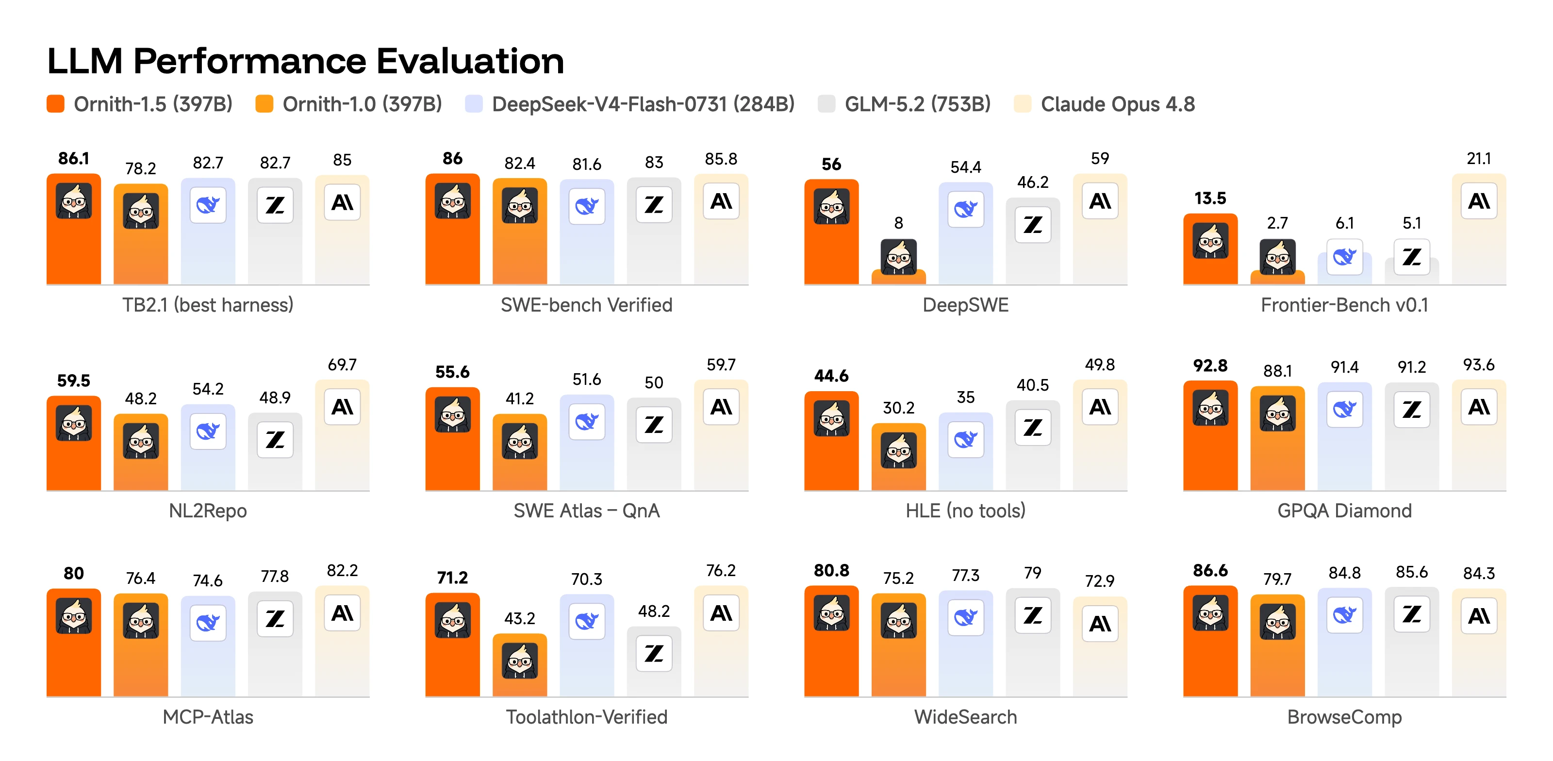
Beyond meeting the criteria I proposed above, they are the closest thing to a production-ready out-of-the-box framework for building extensible web apps that I’ve been able to find in 2026. (But I bet there will be more soon)

There are a handful of things that they provide that you’ll need to build out yourself with other solutions:

Observability

(My day job and personal soapbox)

Both you and your users need visibility into what their code is doing. Cloudflare Workers have OpenTelemetry tracing built into the runtime itself and have first-class primitives that allow you a lot of control over emitted telemetry.

Multi-tenant data storage

While not every extension system needs users to be able to store their own data, this gives users a lot more flexibility.

Give them their very own SQLite database with Durable Object facets. Or give them their own R2 bucket.

Durable Execution

The rise of Temporal et al has shown that a lot of problems benefit from Durable Execution. Dynamic Workflows lets users to take actions over minutes or days, with appropriate retries and backoff.

Source Control

Users probably need to version and iterate on their extensions, and you can’t expect that everyone uses GitHub. Build source control into your product.

Hosted LLMs

Users can use LLMs to help draft their extensions, but you can also expose LLMs through Workers AI so users can use them in their extensions (with appropriate token budgets and rate limits).

export async function analyzeArticle(env: Env, article: Article) {
  return result = await env.AI.run(
    messages: [
      {
        role: "system",
        content: "Decide whether the supplied article talks about cute kittens.",
      },
      {
        role: "user",
        content: article.text,
      },
    ],
  )
}

Self-hosting JavaScript Tooling

A lot of JavaScript tooling is itself written in JavaScript, which means that building and testing extension code might not need a separate container or VM.

import { transform } from 'sucrase';

export function transpileUserCode(source: string): TranspileResult {
  try {
    const result = transform(source, {
      transforms: ['typescript'],
      disableESTransforms: true
    });
    return { type: 'success', code: result.code };
  } catch (err) {
    return { type: 'failure', error: String(err) } };
  }
}

Demo Time

As I was writing this post I thought “What if I turned my static blog into the world’s smallest vibe-coding platform?”5

I wanted to include a guide to working with Dynamic Workers and some cool demos, but this blog post is already way too long. I split that out into a guide to Working with Dynamic Workers but still wanted to embed the final demos here.

The demo’s harness is based around the idea of a customizable scraper. Given a URL, it will fetch the contents (unless they block Cloudflare), and pass those contents and a few utilities to the user’s code. See the guide for a full explanation.

All of the examples run on Cloudflare Workers, and the source is editable. Modify any of them to run your own script, or if you want to write your own choose “Write your own” and there’s an LLM prompt to get you started.

Each example runs through the same harness, but exercises a different combination of libraries and capabilities. Choose one, pick a suggested URL, or your own, and hit Run.

Here be dragons

One last thought.

I’ve worked at platforms for almost a decade. I don’t mean to make “turn your app into a platform” sound easy. Platforms are hard: hard to design, hard to run, hard to debug.

Exposing APIs to customers means a lot of upfront thought, and long-term support (though maybe LLMs can make this a lot easier?).

But they are also really fun, both as a user and a creator. You can be truly surprised by the creativity of your users as they do things that you never considered or would have even thought possible.

Platforms are hard, but it’s worth it.

Appendix

Some things that were influential in drafting this blog post:
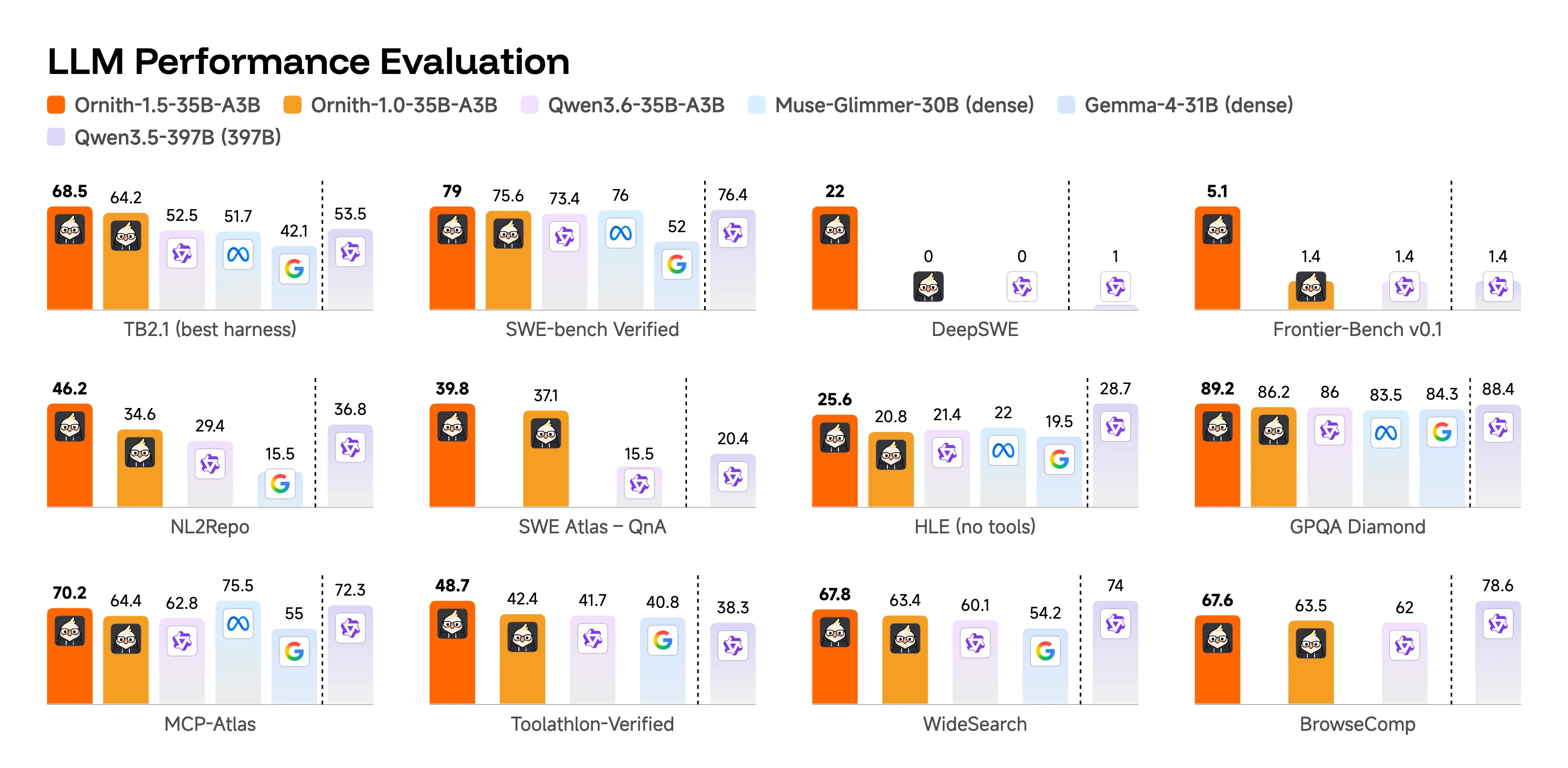
Footnotes

  1. I suspect that even in a fully LLM-accelerated world participation equality is still going to be A Thing. A small percentage will author most of the extensions in any given ecosystem, no matter how easy we make it.
  2. If you squint, vibe coding platforms are kind of a generic version of this, except instead of providing custom functionality for your organization, they provide generic data storage and hosting. I expect they will start to add this kind of customized hosted access as they start selling to Enterprise.
  3. This completely glosses over a need to sandbox UI on the client side where custom code can access potentially sensitive data. That topic deserves its own post.. Or point your robot at cloudflare-os and ask it how it’s done there.
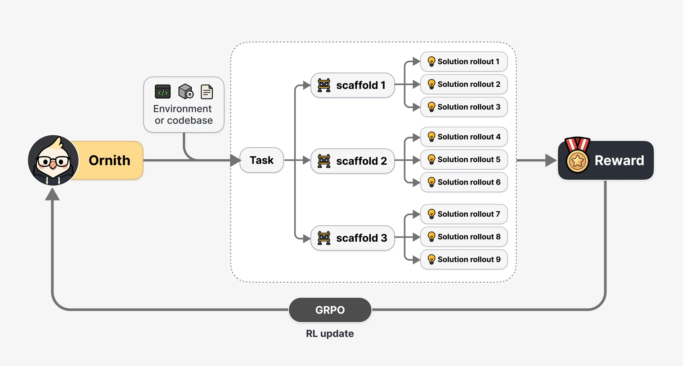
  4. If you’re familiar with Workers, you might be thinking “this looks a lot like bindings…”. Yes! Bindings and Service Workers work on an Object Capability RPC system. You can think of exposing capabilities to users as generating bindings for your particular service.


  5. You’ll have to bring your own vibes though. I decided “expose free LLM usage to the internet” was probably not in my best financial interest.
The Daily Front Page 18 of 30
Wednesday, August 19, 2026 The Daily Front No. #260819 — Bun Under Review
article

Bun 1.4 Rust rewrite is not looking good?

by tipiirai·▲ 137 points·88 comments·tipiirai.com ↗
The last three months have not looked good for Bun.

I care about Bun. I have been rooting for it since the initial release in 2022. I switched all my development from Node to Bun. I used it in the development of the Nue framework and now with my new project Hertta.

The last three months have not looked good for Bun. It started as one of the most impressive individual engineering projects I have seen, but has now turned into this weird AI-powered creature with continuous false promises and an increasingly frustrated community.

In the next version of Bun

In the next version of Bun used to be a positive tweet to watch for. For years it meant a feature had been implemented, tested, and would ship in a few days. This changed after the Rust rewrite. Now the posts are false promises about the upcoming release:

Jun 24Bun v1.4 ships July 7th.

Jul 4Bun v1.4 hopefully Tuesday

Jul 7(The date passes)

Jul 14In the next version of Bun

Jul 20In the next version of Bun

Jul 29Bun v1.4 fixes over 3000 issues over v1.3

Aug 1In the next version of Bun

Aug 4In the next version of Bun

Aug 71 more PR to merge then it’ll be time for Bun v1.4

Aug 13Bun v1.4 is compiling.

Aug 15Bun v1.4 is delayed until Monday

Aug 17Let’s say tomorrow

It’s now three months and counting since the last stable release, the longest gap in Bun’s history since 2022. Nothing unusual there. Software slips, that’s normal. It’s just that an account which used to communicate with real dates and real numbers has switched to vibing. And the user reaction is what you’d expect after constant false promises:

"

@jarredsumner okay I’m editing blog post it’s mostly done if I say a date you won’t believe me but let’s say tomorrow

"

We totally believe in you, Jarred

Rejoice fellas, tomorrow in Jarred Standard Time zone means we have a new blog coming next week.

You won’t care, but personally I am switching to go now. It’s not even funny, you are just stringing your users along again and again.

How can we believe you? You always make promises that you can’t keep, tomorrow, next week, Monday...

If you need 2 months to release it you can just say that instead of saying you’ll ‘release it tomorrow’ every week

Bun on GitHub

The Bun 1.4 rewrite is a big bet on AI. In the past month, 15.8k commits came from robobun, 1.6k commits from autofix-ci[bot], and 790 commits from Jarred.

"6 months ago, most of Bun’s PRs came from people prompting Claude. Nowadays, most of Bun’s PRs come from Claude prompting Claude.

Jarred Sumner

"

The project has over 5k open pull requests, which is the largest number of pull requests I’ve seen. For comparison, OpenClaw has 2.2k, and React has 441. GitHub recommends staying under 1,000 open PRs against a single branch before mergeability checks start timing out.

The biggest worry is, of course, the code itself. In the early days Jarred’s work was inspirational. I thought he was a true Zig talent, until I read Zig creator Andrew Kelley’s thoughts on the Bun rewrite:

"We became increasingly horrified at the programming practices we saw in Bun’s codebase. Hacks on top of hacks. Abuse of assertions. Jarred was already writing slop well before he had access to LLMs.

Andrew Kelley

"

What was the problem with Zig?

This rewrite is the most closely watched real-world test of whether AI agents can take over a production codebase with a human mostly directing rather than reading. Anthropic’s own reputation is also on the line: if this goes well, it is real proof of what agentic coding can do. If it goes badly, it will send a signal in the opposite direction.

The number of unsafe blocks in the Rust code suggests the rewrite did not deliver the memory safety that was given as the reason for doing the rewrite in the first place. Instead this rewrite feels more like an Anthropic ad.

And was Zig really the problem? Bun’s early identity was built on Zig: its performance, its fast compile times, its low friction, its direct memory control with a small team.

It feels like Jarred and Anthropic decided early on that this was going to be written in Rust, and used Zig’s memory issues as the excuse to let the world know how powerful Claude is. A rewrite like this would make great headlines, and it certainly did. Now we’re looking at the long tail of issues from the rewrite they didn’t prepare for.

Maybe Bun should have put that same AI-assisted effort into disciplined, human-understood Zig instead of a full language change. I never saw Jarred seriously engage with this option.

And ‘tomorrow’ has come and gone. Still no v1.4.

¯\_(ツ)_/¯

The Daily Front Page 19 of 30
Wednesday, August 19, 2026 The Daily Front No. #260819 — Keeping the Cluster Alive
article

How Kubernetes Probes Work

by cyndunlop·▲ 125 points·22 comments·ngrok.com ↗
How they can make your application more resilient.

I’m going to show you, really show you, how probes work in Kubernetes. How they can make your application more resilient, and how they can help you prevent avoidable mistakes. Like restart loops that take hours to recover from, and dropping requests during rollouts.

Every interactive demo in this post uses webernetes, my partial port of Kubernetes to TypeScript. It contains more than 100,000 lines of ported Kubernetes Go code to run a simulated cluster right here in your browser. I verified the behaviour of these demos against k3s and managed to find a bug in Kubernetes! More on that later.

What you will learn

  1. The 3 types of probe and what they’re for.
  2. How to configure and combine them.
  3. How common misconfigurations fail.
  4. How probes affect Deployment speed.

A pod without probes

I want to run a pod with a single container. Here’s its manifest, pod-a.yaml:

pod-a.yaml

1apiVersion: "v1"2kind: "Pod"3metadata:⋯4  name: "pod-a"5spec:⋯6  containers:⋯7    - name: "app"⋯8      image: "my-app:latest"

This image, my-app:latest, spends a few seconds initialising before listening on port 8080. You will see this below when you click restart to send the container a signal, causing it to crash and get started back up by Kubernetes. You can pause or reset any demo at any time.

After the first crash, the container restarts straight away. After the second, Kubernetes imposes a CrashLoopBackOff on it before starting it again. By default this delay is 10 seconds, doubling with each crash up to a maximum wait of 5 minutes. I shortened it to 3 seconds for this demo.

In both cases, Kubernetes considers the container Ready as soon as it starts, even though we know it’s not. It’s still doing startup work and not listening on port 8080.

Next I’ll add pod-b, which sends a request to pod-a every 2 seconds. Throughout the post, you can think of pod-b as any source of client traffic: an ingress controller, a load balancer, inter-service requests, etc.

If you restart pod-a in the demo below while a request is on its way, that request will fail.

From the moment you restart the container until its startup work finishes, requests will fail, even though the container is considered Ready! This is not what I want. I need Kubernetes to know when pod-a is ready to receive traffic.

For this, Kubernetes gives us probes. Probes are periodic checks sent to containers to determine their health. They come in three flavours:

  • Startup probes determine whether my application inside the container has started.
  • Readiness probes determine whether my application is ready to receive traffic.
  • Liveness probes determine whether my application needs to be restarted.

It sounds like startup probes are best suited to the problem I showed you in the demos above, so let’s start there.

Startup probes

Below, I’ve added a startup probe to pod-a.yaml:

pod-a.yaml

1apiVersion: "v1"2kind: "Pod"3metadata:⋯4  name: "pod-a"5spec:⋯6  containers:⋯7    - name: "app"⋯8      image: "my-app:latest"9      startupProbe:⋯10        httpGet:⋯11          path: "/startup"12          port: 808013          periodSeconds: 114        failureThreshold: 5

It’s an httpGet probe that sends a GET /startup request to the pod on port 8080. Status codes 200-399 count as a success. This happens every periodSeconds seconds, and is allowed to fail failureThreshold consecutive times before Kubernetes kills the container. This gives my container ~5 seconds to complete its startup work.

Kubernetes also supports tcpSocket, exec, and grpc probes. These establish a TCP connection, run a command inside the container, or call the gRPC health-checking protocol to establish container health. You can read about them in the Kubernetes documentation. I’ll be using httpGet throughout this post.

Probes are sent by a process called the kubelet. Each node in the cluster has its own kubelet, and it’s the kubelet’s job to make sure the right pods are running and being probed for each node.

When you restart pod-a below, it now shows as NotReady. Kubernetes is now aware that pod-a hasn’t initialised yet. It only becomes Ready after the first startup probe succeeds.

NotReady is the default for pods with containers that have a startup probe. However, even when not ready, pod-b still sends requests to pod-a and those requests still fail during the container’s startup period. This is because I’ve configured pod-b to send requests directly to pod-a’s IP address, which bypasses the readiness mechanism.

I'm lying a bit about NotReady

Technically Kubernetes doesn’t have a NotReady condition, it has a Ready condition that can be True, False, or Unknown. I’m referring to it as NotReady because it was shorter than having Ready=True or Ready=False in the demos.

To fix these failed requests I need to graduate to a more production-grade setup: multiple copies of pod-a with requests load-balanced between them. I’m going to create a ReplicaSet configured to run 2 replicas of pod-a and a Service to load balance between them.

replica-set-a.yaml

1apiVersion: "apps/v1"2kind: "ReplicaSet"3metadata:⋯4  name: "replica-set-a"5spec:⋯6  # Run 2 copies of the pod defined under `template`.7  replicas: 28  selector:⋯9    matchLabels:⋯10      # Consider pods with this label to be part of this replica set.11      app: "pod-a"12  template:⋯13    metadata:⋯14      labels:⋯15        app: "pod-a"16    spec:⋯17      # The same pod spec from before.18      containers:⋯19        - name: "app"⋯20          image: "my-app:latest"21          startupProbe:⋯22            httpGet:⋯23              path: "/startup"24              port: 808025            periodSeconds: 126            failureThreshold: 5

service-a.yaml

1apiVersion: "v1"2kind: "Service"3metadata:⋯4  name: "service-a"5spec:⋯6  selector:⋯7    # Load-balance between pods that have this label.8    app: "pod-a"9  ports:⋯10    # Send requests to this port on the pods.11    - port: 80⋯12      targetPort: 8080

pod-b will from now on send requests to the DNS name Kubernetes creates for the Service, in this case service-a.default.svc.cluster.local, instead of directly to an individual pod. Kubernetes uses a pod’s Ready condition to include or exclude it from Service load balancing.

Below you can click the restart button to crash only the top container. Notice that when the top container is starting up, requests are always sent to the bottom container. When a container is NotReady, it marks the whole pod not ready and it won’t get traffic from any Services it is part of.

Despite this, requests can still fail if they’re in-flight when you restart the top container. This happens because the restart button crashes the container abruptly. It doesn’t get a chance to finish in-flight requests.

The better thing to do here is delete the pod and rely on the ReplicaSet to bring up a new one. This is better for 2 reasons:

  1. Kubernetes gives pods a 30-second termination grace period by default, which I’ve configured to 2 seconds in this post so you don’t have to wait. When deleted, pods are considered terminating and Kubernetes removes them from any Services they’re part of. They won’t receive any new requests.
  2. ReplicaSets don’t count terminating pods as active replicas, so they create replacements as soon as the deleted pod is terminating.

Together, graceful termination and the startup probe keep requests away from containers that are starting or stopping. In this next demo, clicking delete won’t cause any requests from pod-b to fail.

There’s always a pod ready to service a new request, making it safe to delete pods without interrupting user traffic.

How does this grace period actually work?

When you delete a pod, the kubelet first sends a SIGTERM signal to the container, then terminationGracePeriodSeconds later it sends a SIGKILL if the container is still running. The Kubernetes docs on pod lifecycle contain all of the gory details.

In this post, my containers are configured to exit 1 second after receiving the SIGTERM. I chose this because I know it’s long enough for them to finish any in-flight requests. When configuring this on your own pods, make sure you leave enough time for your longest-running requests to finish.

How to misconfigure a startup probe

Earlier I mentioned that I’m giving my pod ~5 seconds to complete its startup work by setting failureThreshold to 5 with a periodSeconds of 1. Choose these values on your own containers carefully. Too little time can cause a container to crash-loop.

Setting the failureThreshold below will restart the container with the new value. Set it to 1 or 2 and see what happens.

After a few restarts, pod-a is put in CrashLoopBackOff. The startup probe never gives the container enough time to start, so this demo crash-loops until you set failureThreshold back to 3 or above. When configuring this for your own containers, choose values that allow for your worst-case startup time.

Readiness probes

After any startup probe succeeds, readiness probes monitor the container for the rest of its life. Failing a readiness probe marks the container NotReady and removes it from receiving requests for any Service it is part of.

I’ve modified pod-a.yaml to have just a readiness probe for now:

pod-a.yaml

1apiVersion: "v1"2kind: "Pod"3metadata:⋯4  name: "pod-a"5spec:⋯6  containers:⋯7    - name: "app"⋯8      image: "my-app:latest"9      readinessProbe:⋯10        httpGet:⋯11          path: "/ready"12          port: 808013          periodSeconds: 314        failureThreshold: 115        successThreshold: 1

I’m sending it to the /ready endpoint every 3 seconds. After a single failure, the container gets the NotReady condition. Switch /ready in the demo below from 200 to 503 and watch the container become not ready.

Out-of-band probing

Reset the demo above and watch the first few seconds again. Readiness probes are sent way more often than every 3 seconds. What gives? The Kubernetes docs say this:

While a container is not Ready, the readiness probe may be executed at times other than the configured periodSeconds interval. This is to make the Pod ready faster.

Wonderfully vague. In the work I did on webernetes I found that there are many things that can trigger these out-of-band probes. Without going too into the weeds, most updates to the pod while the container is NotReady can trigger an out-of-band probe. Things like updating annotations or status, for example. Many things can be updating pods that you may not be aware of.

Fun to know, but ultimately not something you should rely on in practice.

The demo above sets failureThreshold and successThreshold to 1, but I don’t want a single transient failure to remove my pods from their Services. Below I’ve set the thresholds to 2. Set /ready to 503 again and notice it now takes 2 failures before the container becomes NotReady.

You may notice here that when flipping from ready to not ready, an out-of-band probe can be fired. This is for the same reasons as before. The pod is NotReady and its status just got updated.

By default successThreshold is 1 and failureThreshold is 3. Generally good defaults that I don’t recommend changing unless you have a great reason.

Why do we need startup probes if we have readiness probes?

The demos above only use a readiness probe. Probing starts straight away and doesn’t succeed until my container has finished its startup work. This is exactly the job my startup probe was doing, so why do we need both probe types?

A few good reasons:

  1. Startup probes delay readiness and liveness starting until initialisation is complete.
  2. They allow startup to have a separate periodSeconds and failureThreshold, so slow initialisation can be probed more frequently than steady-state readiness and liveness.
  3. Repeated startup failures kill the container and apply its restart policy. Readiness failures don’t. A restart could help a stuck container become ready.

You can use multiple probes at the same time. For example, I might send a startup probe every second to detect initialisation quickly, then slow down to every 5 seconds for my readiness probe to reduce steady-state probe load on the container and kubelet.

pod-a.yaml

1apiVersion: "v1"2kind: "Pod"3metadata:⋯4  name: "pod-a"5spec:⋯6  containers:⋯7    - name: "app"⋯8      image: "my-app:latest"9      startupProbe:⋯10        httpGet:⋯11          path: "/startup"12          port: 808013          periodSeconds: 114        failureThreshold: 515      readinessProbe:⋯16        httpGet:⋯17          path: "/ready"18          port: 808019        periodSeconds: 5

Readiness probes don’t start until the startup probe succeeds. I’ve started the demo below paused so you can see it from the start. Hit the play button when you’re ready, and press reset if you want to start again from the beginning.

This guarantee, that readiness probes don’t start until startup succeeds, allows me to check startup-specific things in the /startup endpoint. I could make sure initial configs have been loaded, caches have been pre-warmed and so on. In practice, startup probes are less commonly used than readiness probes. It’s nice to know they’re there as an option if I need them, though.

If you do find yourself wishing readiness probes could restart containers, though, I have just the thing for you.

Liveness probes

The final probe type is the liveness probe. This probe works just like the readiness probe, but instead of marking a container NotReady when it reaches its failureThreshold, the liveness probe kills the container. Kubernetes then applies the Pod’s restartPolicy, which defaults to "Always" and means a killed container will be restarted.

pod-a.yaml

1apiVersion: "v1"2kind: "Pod"3metadata:⋯4  name: "pod-a"5spec:⋯6  containers:⋯7    - name: "app"⋯8      image: "my-app:latest"9      startupProbe:⋯10        httpGet:⋯11          path: "/startup"12          port: 808013          periodSeconds: 114        failureThreshold: 515      livenessProbe:⋯16        httpGet:⋯17          path: "/live"18          port: 808019        periodSeconds: 220        failureThreshold: 1

This helps when the container can’t recover on its own, such as when its main thread has deadlocked or a critical background thread has died. If I can reliably detect these conditions, I can fail the liveness probe and rely on Kubernetes to restart the container.

The demo below shows pod-a getting sent startup probes until it finishes its startup, after which the liveness probes begin. Set the /live endpoint to return 503 to see the container get restarted.

There's something wrong with the demo above...

You might notice that when you set the /live endpoint to 503, an odd sequence of events happens.

  1. The liveness probe fails.
  2. The kubelet restarts pod-a’s container.
  3. Before the startup probe has a chance to fire, a liveness probe fires and fails because the container is still in startup.
  4. The kubelet restarts the container again, before it has a chance to pass its startup probe!

This is a real Kubernetes bug that I found during the making of this post. Liveness probes shouldn’t be firing before the startup probe has succeeded. I reproduced this in k3s, minikube, and kind against the latest Kubernetes at time of writing v1.36.2. The bug appears to have been introduced in v1.35.0. I’ve filed an issue about it and SIG Node have accepted it and marked it priority/important-soon.

Until it’s fixed, please imagine the premature liveness probe never fires. Thank you.

How to misconfigure a liveness probe

It would be a bad idea for my liveness probe to check if my database is healthy. A blip in the database could cause all of my containers to crash-loop if it lasts long enough.

When you take the database down in the demo below, the pod-a liveness probes will fail. After a few failures, each container will go into CrashLoopBackOff. To stress how bad this can be, I’ve made the backoff delay scale like it does in real Kubernetes: 10 seconds at first, doubling for each crash. Go and cause some havoc!

This problem gets worse if clients retry. It hasn’t come up in any other demos so far, but my pod-a containers can only handle 3 requests per second. If they get more than that, they get overloaded and crash! I’ve configured pod-b in the demo below to retry failed requests in a loop, and set the maximum CrashLoopBackOff delay to 5 seconds again. Cause another outage, and see if you can recover from it.

The retries create what’s called a thundering herd, which causes a cascading failure. It doesn’t matter that the database is up, any container that dares to recover gets a laser beam of traffic that kills it again.

Probes, sadly, can’t help me get out of this. I would need to create some way to only let a small percentage of traffic through, allowing the containers time to recover, then ramp back up to full traffic over time. Or if I have control over the clients, for example they’re a mobile app I’ve also created, I could add a backoff delay to the retries. This would slow the traffic growth, making it easier to recover.

The best thing I can do, though, is avoid this mistake in the first place. Fail a liveness probe only when the failure is local to one container and a restart is likely to restore it. Don’t fail on conditions that will be true for all of your containers at the same time.

Probes and Deployments

The last thing I want to touch on is how probes affect Deployments. In Kubernetes, most of a Pod’s spec is immutable. The way to update an immutable field is to create a new Pod and delete the old one. Deployments manage this replacement as a “rollout.”

Let’s take deployment-a.yaml here as an example:

deployment-a.yaml

1apiVersion: "apps/v1"2kind: "Deployment"3metadata:⋯4  name: "deployment-a"5spec:⋯6  replicas: 37  strategy:⋯8    type: "RollingUpdate"9    rollingUpdate:⋯10      maxUnavailable: "25%"11      maxSurge: "25%"12  selector:⋯13    matchLabels:⋯14      app: "pod-a"15  template:⋯16    metadata:⋯17      labels:⋯18        app: "pod-a"19    spec:⋯20      containers:⋯21        - name: "app"⋯22          image: "my-app:latest"23          ports:⋯24            - name: "http"⋯25              containerPort: 808026          startupProbe:⋯27            httpGet:⋯28              path: "/startup"29              port: "http"30            periodSeconds: 131            successThreshold: 132            failureThreshold: 5

I’ve highlighted the strategy because it’s the part that controls how new Pods get rolled out. Deployments start off by creating a ReplicaSet to bring up the replicas I’ve configured. Changing a Deployment’s template after it has been created makes a new, second ReplicaSet configured with this new template. The Deployment then scales up the new ReplicaSet while scaling down the old one, based on the strategy parameters.

Here’s what each strategy parameter means:

  1. type: "RollingUpdate" updates the Pods gradually rather than all at once. If you did want all at once, you would use type: "Recreate". This first scales the old ReplicaSet to 0, then the new one to the configured replicas. This causes downtime, so it’s not the default.
  2. maxUnavailable: "25%" allows floor(3 * 0.25) = 0 unavailable replicas, so all 3 must remain available during the rollout.
  3. maxSurge: "25%" allows ceil(3 * 0.25) = 1 extra pod above replicas during the rollout, so in our case 4 replicas are allowed to exist.

It’s a lot, so clicking deploy below may help you better understand. Remember that the rollout has to keep 3 pods Ready at all times, and is allowed to go up to 4 replicas thanks to maxSurge. Pods that are terminating don’t count as available, so you will see more than 4 replicas at times.

The rollout can only create 1 extra pod, and has to wait for that pod to become Ready before it can kill an old pod. This means that probes play a direct role in how fast a rollout can go. You should see that with the above configuration, it takes about 11 seconds to finish. Also notice that no requests from pod-b fail.

Below, I’ve changed periodSeconds from 1 to 5. See how long it takes to deploy with this longer period.

It now takes about 19-20 seconds for this rollout to complete. Longer startup probe periods delay rollouts because each replacement pod has to wait until it passes the probe. Keep this in mind when tuning your own probes.

Lastly, what happens if I update a Deployment and have no probes at all? In the demo below, you will notice that a rollout will cause a small number of requests to fail because the new containers haven’t finished their startup.

A rollout without probes happens very quickly because each container is considered ready as soon as it starts. This causes a small number of requests to fail because the containers haven’t finished startup yet.

Tips for designing good probe endpoints

Startup

  1. Use them when startup is slow or variable, or you have initialisation work that can get stuck and needs to be restarted.
  2. Probe frequently to detect initialisation quickly. If you do lower periodSeconds, make sure to increase failureThreshold to maintain the total time you wait for startup. Target your worst-case startup time, plus a little headroom.
  3. Take advantage of a separate /startup endpoint if there are checks you can do to be certain initialisation has finished. If not, using the same endpoint as your liveness check is reasonable.

Readiness

  1. Keep this probe cheap and conservative. Fail it only when removing a pod from serving is likely to improve overall service health.
  2. Prefer not to fail readiness based on the status of shared dependencies like database servers and third-party APIs. Include a dependency only when a container truly can’t serve useful traffic without it.
  3. Prefer not to fail readiness in response to high CPU or memory. If your service is near total capacity, removing a replica may cause a cascading failure.

Liveness

  1. Fail this probe only when it’s very likely a container is stuck and a restart will help. If you aren’t sure, return success.
  2. Don’t fail liveness based on the status of shared dependencies like database servers and third-party APIs.
  3. Don’t fail liveness in response to high CPU or memory.

General advice

  1. Keep probes bounded and cheap. Startup probes have a bit more wiggle room than the other two, but they still consume cluster resources that could be spent serving user traffic.
  2. The default failureThreshold is 3. Lower it only when immediate intervention is worth the risk of reacting to a transient failure.

Probe playground

Below is a demo that lets you set whatever probe parameters you want. Changes won’t be applied until you press deploy. It’s surprisingly easy to get yourself into unrecoverable situations, so don’t feel bad about using the reset button.

Conclusion

Probes are tricky to get right. By showing you how they work, and letting you cause some chaos, you’re now better equipped to make informed decisions about your own probes. If you have feedback about this post, or you’re curious about webernetes, I would love to talk to you! Email me at s.rose@ngrok.com.

The Daily Front Page 20 of 30
Wednesday, August 19, 2026 The Daily Front No. #260819 — The Engineering Desk
article

Go 1.27

by database64128·▲ 593 points·158 comments·go.dev ↗

Today the Go team is pleased to release Go 1.27. You can find its binary archives and installers on the download page.

Go 1.27 brings major enhancements across the language, toolchain, runtime, and standard library. Below are some of the key highlights.

Language changes

Go 1.27 introduces three notable updates to the language specification.

First, generic methods are now supported. For example, see math/rand/v2.Rand:

// Prior to Go 1.27, a separate method on Rand had to be added for each type
// (unsigned integer methods omitted for brevity).
func (r *Rand) Int32N(n int32) int32
func (r *Rand) Int64N(n int64) int64
func (r *Rand) IntN(n int) int

// Go 1.27 adds a new generic method that works for all integer types.
func (r *Rand) N[Int intType](n Int) Int

Second, a key in a struct literal may now be any valid field selector for the struct type, allowing fields in nested or embedded structs to be initialized directly:

type Habitat struct {
    Burrow string
}

type Gopher struct {
    Name    string
    Habitat // Embedded struct.
}

// Go 1.27 allows using Burrow as a key directly.
g := Gopher{
    Name:   "Gopher",
    Burrow: "Burrow #42",
}

Finally, function type inference has been generalized to apply in all assignment contexts. Generic functions can now be used without explicit type arguments in composite literals, type conversions, and channel sends:

func GenericFormatter[T any](v T) string {
    return fmt.Sprintf("value: %v", v)
}

type IntFormatter func(int) string

// Go 1.27 infers T = int in composite literals, conversions, and channel sends.
formatters := []IntFormatter{GenericFormatter}
fn := IntFormatter(GenericFormatter)
ch := make(chan IntFormatter, 1)
ch <- GenericFormatter

Tool improvements

  • go fix includes several new modernizers: atomictypes, embedlit, slicesbackward, and unsafefuncs.
  • go doc now supports package@version queries such as go doc example.com/pkg@v1.2.3.
  • go mod tidy now automatically consolidates multiple require blocks in go.mod into a standard direct and indirect two-block structure.

Performance and runtime

Standard library additions

Please read the Go 1.27 release notes for the complete list of changes and details.

Over the next few weeks, follow-up blog posts will cover some of the topics relevant to Go 1.27 in more detail. Check back later to read those posts.

Thanks to everyone who contributed to this release by writing code, filing bugs, trying out experimental additions, and testing release candidates. As always, if you notice any problems, please file an issue.

We hope you enjoy using Go 1.27!

The Daily Front Page 21 of 30
Wednesday, August 19, 2026 The Daily Front No. #260819 — The Engineering Desk
article

Cerebras CS-4

by sunils34·▲ 456 points·268 comments·cerebras.ai ↗

Introducing the all new Cerebras CS-4, a revolutionary rack-scale solution that delivers up to 30x faster inference compared to GPUs, enhanced economics, and a simple path to deploy hyperscale capacity. It is the architecture for frontier AI.

Three WSE-3 Turbos per System

Each wafer delivers up to 2x the speed of the previous generation

Faster Wafer I/O

Scales massive models and enables heterogeneous, disaggregated inference

Nexus Rack-Scale Platform

Enables rapid deployment in hyperscale datacenters

Up to 30x faster than GPUs

Powered by WSE-3 Turbo, CS-4 delivers up to 30x faster inference compared to GPU systems, setting a new record for the fastest inference available in production.

Higher ultrafast throughput

The CS-4 solution shifts the inference Pareto frontier, delivering up to 10x more throughput per watt than CS-3 while generating tokens up to 30x faster than production GPU systems. The result is a system designed to deliver both throughput and interactivity.

Frontier-ready architecture

By reducing wafer-to-wafer interconnect latency to 2 microseconds, CS-4 delivers more than 1,000 tokens per second on models exceeding 10 trillion parameters, preserving interactive decode performance at unprecedented scale.

THE NEXUS RACK-SCALE PLATFORM A MODULAR RACK DESIGN TO ENABLE FASTER DEPLOYMENTS

CS-4 is the first iteration of the new Cerebras Nexus Platform Architecture. It is built around a modular concept with three foundational elements: Compute, Power, and I/O – each with significant innovation to simplify manufacturing, deployment, maintenance, and upgrades.

Modular compute backpack design

Cerebras has fundamentally re-imagined the server. Each Wafer-Scale Backpack is a self-contained assembly that folds the wafer, power conversion, direct liquid cooling, high-speed I/O, and control electronics into a compact 3D package with 50% fewer components. This design simplifies manufacturing and reduces deployment time from days to hours.

High-density power delivery

With power delivery just 0.5 millimeters away from the processor - roughly 100x closer than the roughly 50mm of conventional GPU boards - CS-4 nearly eliminates board-level power loss. This enables the delivery of twice as much power to the WSE-3T, enabling higher operating frequencies and faster token generation.

Next-gen wafer I/O interface

CS-4 introduces a new programmable I/O subsystem that doubles I/O bandwidth and reduces latency, benefitting both aggregated and disaggregated solutions. The Wafer I/O Module also enables wafers to be linked within and across racks without a switch, for wafer-to-wafer latency as low as two microseconds that is key to interactivity for models with tens of trillions of parameters.

THE FASTEST WAFER YET

CS-4 runs on WSE-3 Turbo—the world’s largest and fastest AI processor. Its four trillion transistors and 900,000 AI cores deliver 250 PFLOPS of compute and 43.2 petabytes per second of memory bandwidth.

Twice the compute. Twice the bandwidth. Less than half the latency. A massive leap in AI speed and throughput.

CS-4 by the numbers

First CS-4 shipments begin this quarter. Bring the fastest AI to your data center.

Get started Datasheet

FAQ

What is Cerebras CS-4?

How is CS4 different from CS-3?

How fast is CS-4?

How much throughput does CS-4 provide?

Why is CS-4 well suited for agentic AI?

What is a Wafer-Scale Backpack?

How does the Nexus Platform Architecture simplify hyperscale deployment?

What models and inference architectures does CS-4 support?

The Daily Front Page 22 of 30
Wednesday, August 19, 2026 The Daily Front No. #260819 — The Engineering Desk
article

Palomar: A registry of Lean verified mathematics

by matt_d·▲ 177 points·39 comments·terrytao.wordpress.com ↗

In recent months there has been a proliferation of AI-generated proofs of various old and new results, some of which have been formalized in the proof assistant language Lean. However, checking that a given Lean repository actually proves the claimed statement is somewhat non-trivial, especially for an audience which is not expert in the use of Lean: one has to first check that the claimed formal Lean statements have proofs that typecheck, that the proofs do not contain any “cheats” such as adding additional axioms, and that the formal statements also match (in a semantic sense) the informal description of the claimed results.

To help bring some clarity to this situation, I am happy to announce that Palomar registry of Lean verified mathematics, which is an initiative incubated by the Lean FRO and by ICARM, is now open for submissions. I am serving in several roles on this registry, including on the scientific advisory board, together with Jeremy Avigad, Matthew Ballard, Jaume de Dios, Nestor Guillen, Bryna Kra, Kim Morrison, Ravi Vakil, and Akshay Venkatesh.

A detailed motivation for Palomar can be found here, and further information about Palomar can be found here. A zeroth approximation of what Palomar intends to be is the analogue of a preprint server for Lean proofs. More precisely, Palomar (which is named after the astronomical observatory) is a registry of external Github repositories (or more precisely, “snapshots” of such repositories, as represented by a specific Github commit) containing Lean code adhering to the current best practices for such formalizations, in particular containing

  • A “challenge file” containing a short, human readable description in Lean of the results claimed.
  • A “solution module” containing an (arbitrarily long) proof of the results claimed in the challenge file.
  • A “formalization.yaml” file describing the results in informal language, and also containing a number of other relevant metadata and disclosures.

(There are also some additional technical requirements for the repository which I will omit here.) If a snapshot of a repository is submitted to Palomar, it will check both (a) that the solution module typechecks and proves exactly the results claimed in the challenge file, and that (b) the informal description of the result in the formalization.yaml file appears to match the result claimed in the challenge file, and that the repository meets various minimal standards required for a registry entry. The first check (a) is purely mechanical, using the Lean tool Comparator; the second check (b) is non-deterministic, being performed by a large language model. If a repository passes both checks, it can be registered on Palomar. It is worth stressing that the checks in (a) and (b) fall well short of what a proper human peer review of a submission for novelty, interest, and accuracy would give; in particular, Palomar is not a peer-reviewed journal.

The submission process is thorough, but achievable: as a test, I successfully managed to submit my own recent formalization of the proof of Sendov’s conjecture to Palomar, and also plan to submit some older formalizations to the registry soon.

In any event, the registry is now open for formalizations of both old and new results. Submissions (whether human-generated, AI-generated, or some mixture of both) are welcome; please read the (somewhat detailed) instructions here before starting a submission. (I will however note that modern AI agents are quite helpful in assisting with the mechanical details of the submission, though a human review is still strongly recommended.)

Discussion and feedback on Palomar will occur on this Zulip channel.

The Daily Front Page 23 of 30
Wednesday, August 19, 2026 The Daily Front No. #260819 — The Engineering Desk
repository

Feature Request: Support AGENTS.md

by fg137·▲ 222 points·128 comments·github.com ↗
★ 142,065⑂ 22,785 forks Python

Claude Code is an agentic coding tool that lives in your terminal, understands your codebase, and helps you code faster by executing routine tasks, explaining complex code, and handling git workflows - all through natural language commands.

Codex, Amp, Cursor, and others are starting to standardize around AGENTS.md (https://agents.md/) — a unified Markdown file that coding agents can use to understand a codebase.

By contrast, CLAUDE.md feels too specific to Claude Code. It doesn’t work as well when collaborating with other developers who aren’t using Claude Code.

The Daily Front Page 24 of 30
Wednesday, August 19, 2026 The Daily Front No. #260819 — Proofs, Patients, and Public Life
The Daily Front Page 25 of 30
Wednesday, August 19, 2026 The Daily Front No. #260819 — Proofs, Patients, and Public Life
article

Civic Hygiene – avoid building technologies that could be used by a police state (2013)

by felineflock·▲ 428 points·308 comments·shkspr.mobi ↗

Imagine, just for a moment, that the Government wanted to keep a record of everyone's sexuality. They need to know this detailed demographic data because it will be highly useful in civic planning. It will help them work out what provision needs to be made for sexual health services, how many children are likely to be born, how many schools to build, etc.

You trust the Government, you voted for them, you and your friends have nothing to hide with regards to your sexuality.

But! Shock horror! After creating the database, the Government loses the election and the homophobes at UKIP get in to power!

Now they have a database of every gay in the village, and can harass then, try to "cure" them, or make their lives a living hell.

Far fetched? Not really. With Cameron's inane web filtering plan, the "black boxes" in ISPs which can record every click you make, and the selling of the your NHS details to private parties, we're in a situation where a malicious government could cause serious damage to us.

The security expert Bruce Schneier wrote a wonderful article for CNN on how the existing surveillance state is leading to disastrous breaches of our private information. He concludes by saying:

It's bad civic hygiene to build technologies that could someday be used to facilitate a police state.

-- Bruce Schneier on CNN

We have to be careful that the apparatus we build cannot easily be misused for evil purposes. Sure, even an innocuous toaster can be weaponised if someone is willing enough, but we should not fall into the trap of making systems which can easily be turned against the people.

It's probably sensible to build a database of which car belongs to which owner - it has an important civil use and would be hard to abuse (although not impossible).

Should we have a national database of, say, religious beliefs? Almost instinctively the answer is no. The memories of fascist dictators haunt our collective consciousness. We have seen countless times how race and religious identity become death penalties. We wouldn't countenance it.

Civic hygiene isn't about saying we distrust our current government - it's about not trusting the next government.

The Daily Front Page 26 of 30
Wednesday, August 19, 2026 The Daily Front No. #260819 — Proofs, Patients, and Public Life
article

Mathematics in the age of AI

by jonbaer·▲ 157 points·185 comments·arxiv.org ↗

Abstract

An essay, based on a public lecture delivered at the 2026 International Congress of Mathematicians, on how the mathematical community might respond to the arrival of artificial intelligence tools that are capable of performing research-level mathematical tasks. Rather than debating the capabilities of such tools, we condition on the hypothesis that these capabilities will arrive, and examine instead a question that is orthogonal to it: what the goals and values of mathematical research actually are. The problem-solving component of mathematics is used as a case study.

The Daily Front Page 27 of 30
Wednesday, August 19, 2026 The Daily Front No. #260819 — Late Cards: Devices and Platforms
article

Air Theremin – A browser theremin you play by waving at your webcam

by gurov·▲ 269 points·92 comments·theremin.bizibah.com ↗

Play it in mid-air, two ways. HANDS — wave both hands at the camera: spread them apart for volume, raise them for pitch, lean back to soften the tone, put your palms together for silence. A laptop webcam does just as well as a phone. GYRO — on a phone, tilt it instead: left-right sets volume, forward-back sets pitch, and the whole range lives inside the frame (tilt the marker outside it to cut the sound). With neither sensor nor camera, the mouse drives it. Press START — on a phone, hold it steady and it calibrates to your grip.

The Daily Front Page 28 of 30
Wednesday, August 19, 2026 The Daily Front No. #260819 — Also on the Front Page
The Daily Front Page 29 of 30
Wednesday, August 19, 2026 The Daily Front No. #260819 — Colophon

That's the Front for Today

Issue No. #260819 — Wednesday, August 19, 2026 — went to press 2026-08-20 at 07:29 UTC.

About This Magazine

The Daily Front is a daily digital magazine assembled from the stories that reached the front page of Hacker News on Wednesday, August 19, 2026. Headlines, points, and comment counts are recorded as they stood at press time. All articles remain the property of their original authors — every piece links back to its source and its discussion thread.

How It Was Made

Fetched, cleaned, and typeset by an automated pipeline. An editor model laid out the pages, chose the highlights, and briefed the cover illustrator — 31 model calls and 285k tokens in total. Set in Jacquard 12, Playfair Display, Source Serif 4, and IBM Plex Mono, all served via Google Fonts under the SIL Open Font License.

The Cover

The cover illustration was commissioned with this prompt:

A single expansive scene inside a dimly lit modern workshop that merges into a city skyline: a hand adjusts a sleek computer mouse on a workbench while glowing circuit wafers, a compact server rack, a weather balloon drifting above distant rooftops, and a smartphone with its circuitry exposed share the same physical space. In the background, a researcher studies a luminous map made of coastlines and geometric lines, while clean-air trees and a child’s bicycle sit near an open window. The scene conveys local control, AI infrastructure, public technology, and human consequences, with no text, letters, logos, or symbols.

Render the cover as analog television interference turned into editorial art: dense charcoal-and-ink snow, bent vertical hold, horizontal signal tears, and controlled chromatic bleeding should obscure—but not erase—one recognizable continuous scene emerging through the static. Preserve the dim modern workshop merging into the skyline, with the hand adjusting the sleek mouse on the workbench, glowing circuit wafers, compact server rack, drifting weather balloon above rooftops, exposed-circuit smartphone, researcher examining the luminous coastline-and-geometric-line map, and clean-air trees with the child’s bicycle by the open window, all sharing one physical space and conveying local control, AI infrastructure, public technology, and human consequences. Use a deliberate palette of near-black graphite, electric cyan, acid green, and restrained coral-red interference, with luminous cyan-green highlights bleeding through the noise; no text, letters, logos, or symbols.

Absolutely no text, letters, numbers, readable symbols, or logos anywhere in the image.

Production Ledger

StageModelCallsTokens InTokens Out
extractgpt-5.6-luna 28 179,683 78,025
layoutgpt-5.6-terra 1 19,059 2,294
covergpt-5.6-luna 1 365 223
covergpt-image-2 1 322 5,488

The Publisher

Published by Johnny.

Support the Press

If The Daily Front brightens your morning, consider supporting its publisher.

Credits & Contact

All content — articles, posts, comments, and the images within them — belongs to its original authors and is reproduced here to point readers back to the source. Full credit goes to those creators; every item links to its original and its Hacker News discussion.

If you are an author and would like your content removed from an issue, write to hi@johnnys.page and it will be taken down.

Feedback is always welcome at the same address: hi@johnnys.page.

Credit where credit is due.

Every page of this issue began as someone else's work — these are the original sources, linked in full.

  1. OpenLogi by amatheus — openlogi.org·HN discussion ↗
  2. A joke domain purchase turned in geopolitical warfare by kareiva — sprocketfox.io·HN discussion ↗
  3. OpenRouter is joining Stripe by rvz — openrouter.ai·HN discussion ↗
  4. Remote workers report the highest well-being in study of 7,700 employees by downbad_ — colorado.edu·HN discussion ↗
  5. Geolocating a random island using geometry and CUDA programming by yassa9 — yassa9.github.io·HN discussion ↗
  6. Children's stunted lungs show recovery in ultra low emission zone by dabinat — bbc.com·HN discussion ↗
  7. Sticky wage norms and the real wage cost of unexpected inflation by jplusequalt — bfi.uchicago.edu·HN discussion ↗
  8. PostgreSQL for Everything by karlmush — raphaelbauer.com·HN discussion ↗
  9. Unsloth Dynamic 3.0 GGUFs by jonesy827 — unsloth.ai·HN discussion ↗
  10. The Mojo language (by Modular, now Qualcomm) is now open-source by flaburgan — modular.com·HN discussion ↗
  11. Unlocking a locked/deactivated e-waste Cricut Maker by 1e1a — sprocketfox.io·HN discussion ↗
  12. Ornith-1.5: From Self-Scaffolding to Self-Improvement by CommonGuy — ornith.ai·HN discussion ↗
  13. Police officer used Flock cameras to track estranged wife 717 times by speckx — wsbtv.com·HN discussion ↗
  14. Opus 5.0 drives incoherence into the stratosphere by Bluestein — github.com·HN discussion ↗
  15. Show HN: Automatically detect and patch walking-dead states in Sierra games by wkfauna — github.com·HN discussion ↗
  16. Extensible Software in the age of LLMs by coloneltcb — jeremymorrell.dev·HN discussion ↗
  17. Bun 1.4 Rust rewrite is not looking good? by tipiirai — tipiirai.com·HN discussion ↗
  18. How Kubernetes Probes Work by cyndunlop — ngrok.com·HN discussion ↗
  19. Go 1.27 by database64128 — go.dev·HN discussion ↗
  20. Cerebras CS-4 by sunils34 — cerebras.ai·HN discussion ↗
  21. Palomar: A registry of Lean verified mathematics by matt_d — terrytao.wordpress.com·HN discussion ↗
  22. Feature Request: Support AGENTS.md by fg137 — github.com·HN discussion ↗
  23. Moderna reports first positive Phase 3 for mRNA neoantigen therapy in melanoma by heydenberk — twitter.com·HN discussion ↗
  24. Civic Hygiene – avoid building technologies that could be used by a police state (2013) by felineflock — shkspr.mobi·HN discussion ↗
  25. Mathematics in the age of AI by jonbaer — arxiv.org·HN discussion ↗
  26. Air Theremin – A browser theremin you play by waving at your webcam by gurov — theremin.bizibah.com·HN discussion ↗
  27. Devices with GrapheneOS support should be available in 2027 by exceptione — grapheneos.social·HN discussion ↗
  28. Google has stopped pushing Git tags for some Android source code by Animux — grapheneos.social·HN discussion ↗
  29. Casio F-B100W-1A by __fst__ — casio.com·HN discussion ↗
  30. Meta's blockbuster trial draws parallels to big tobacco by newsomix9xl — economist.com·HN discussion ↗

Browse all issues in the archive →