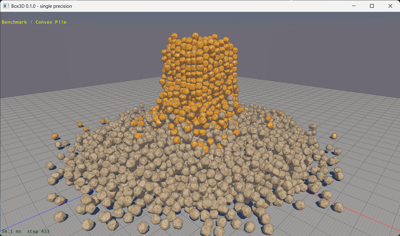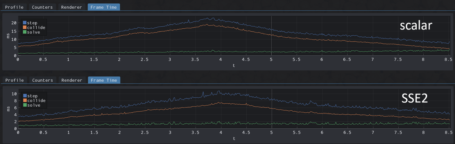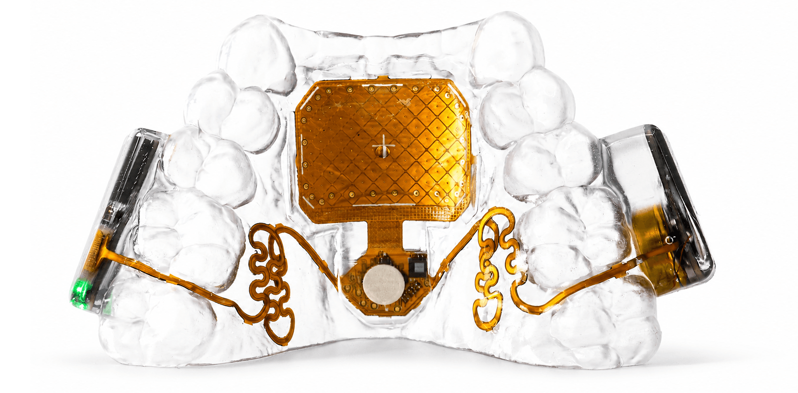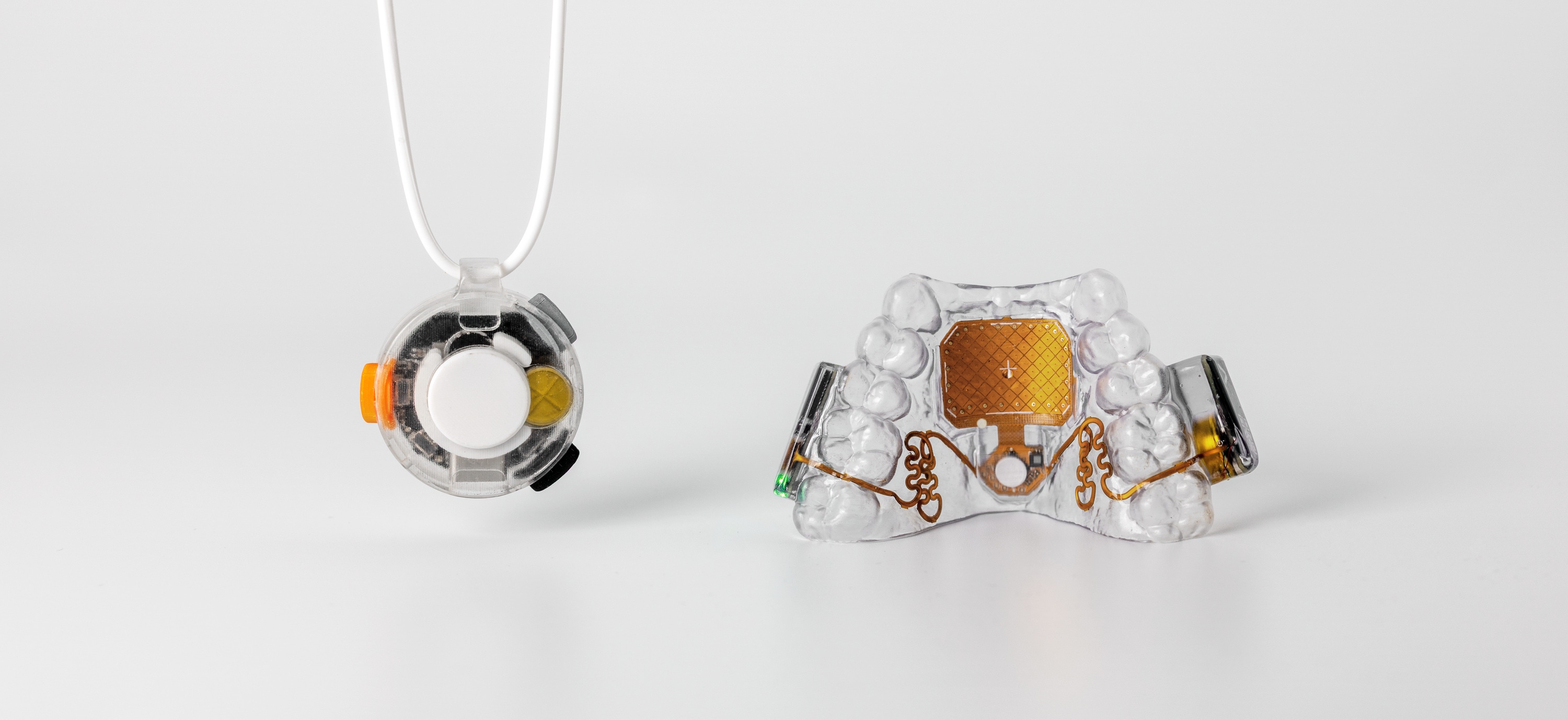
Cover illustration

TheDaily Front

Issue No. #260725 Saturday, July 25 2026 #260725 — SATURDAY, JULY 25, 2026
Security locks the side door while the robots argue over who is smartest.
Saturday, July 25, 2026 The Daily Front No. #260725 — Contents
30stories
8,184points
3,401comments
222kllm tokens
Assembled with 29 model calls — 152,274 tokens read, 69,408 written.

Highlights

Android may soon restrict on-device ADB

A proposed Android ADB restriction ignited a fierce argument over security, ownership, and the shrinking space for power users.

Open-weight AI is having its Kubernetes moment

Open-weight AI advocates warn that the next platform war may be won or lost on interoperability rather than raw benchmark numbers.

The new rules of context engineering for Claude 5 generation models

Claude 5’s context lessons suggest a strange new rule for agents: say less, trust more, and let the model infer the rest.

Building a Tiny 3D Renderer for a Tiny Handheld

A miniature 3D renderer for the Playdate shows how constraints can become an aesthetic rather than an obstacle.

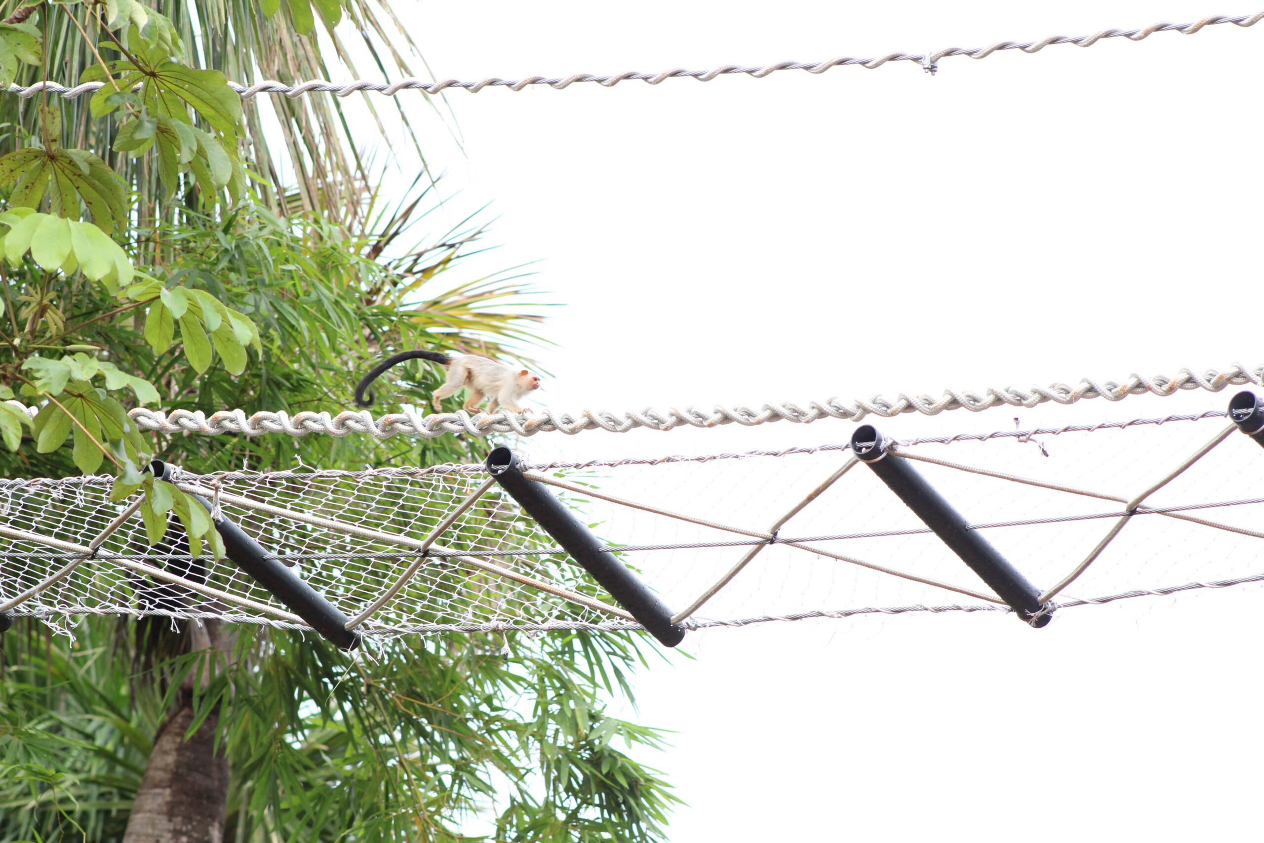
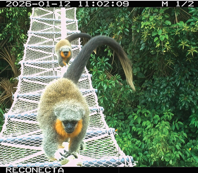
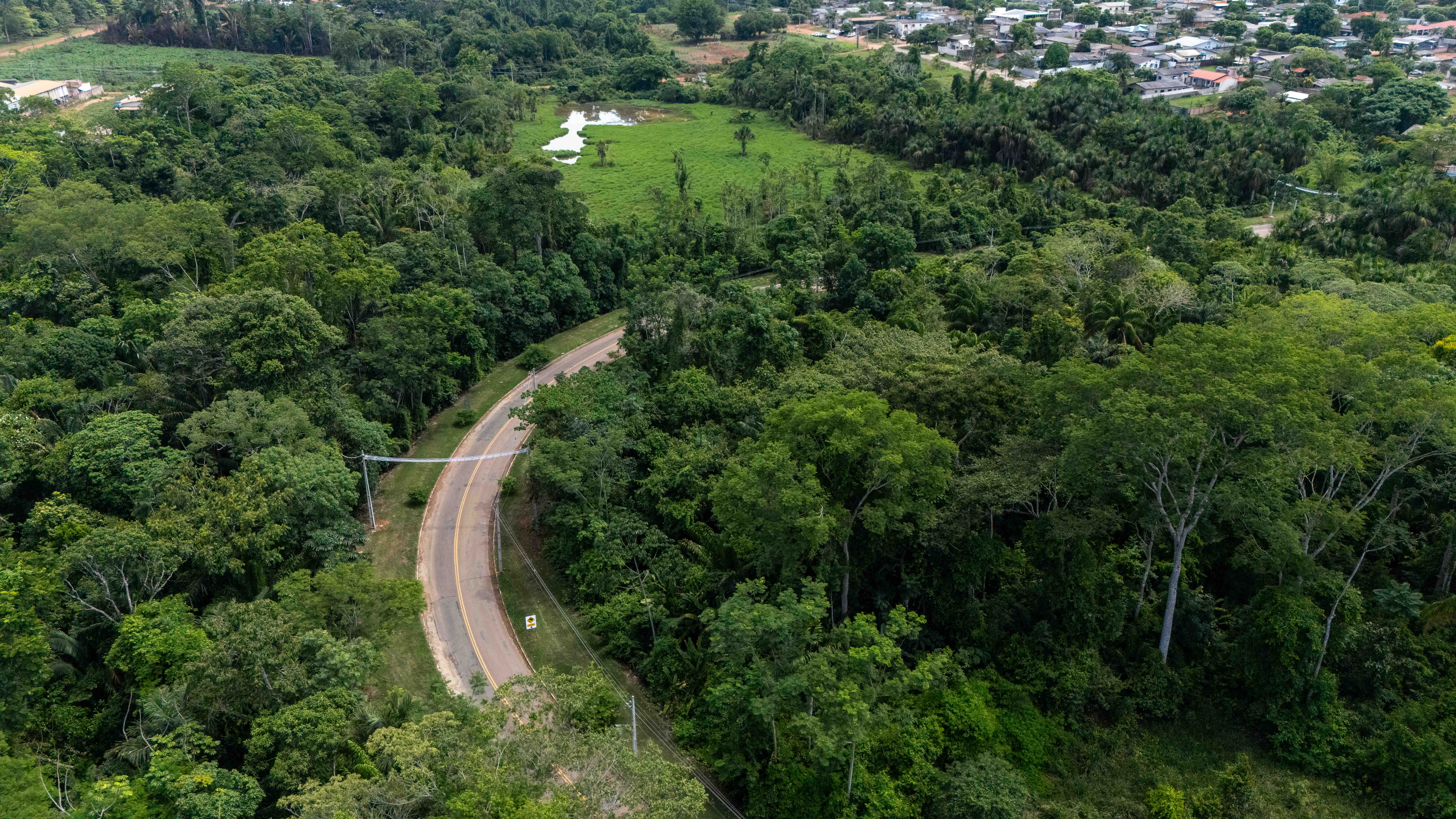
Zero roadkill as Amazon canopy bridges secure 15,000 crossings

Amazon canopy bridges offer a rare conservation headline with measurable success: thousands of safe crossings and no roadkill.

From the Editor

The day’s front page finds the old bargain of computing under fresh strain: users ask to tinker, vendors answer with locks, and the machines in the back room grow ever more clever. Yet amid the policy fog there is still delight—tiny renderers, stolen buttons, whale bubbles, and the stubborn craft of making things work.

  1. Android may soon restrict on-device ADB3
  2. Opus 5 is currently #1 on Artificial Analysis Intelligence Leaderboard4
  3. Open-weight AI is having its Kubernetes moment5
  4. The new rules of context engineering for Claude 5 generation models6
  5. UK AISI / Caisi Preliminary Assessment of Kimi K3's Cyber Capabilities7
  6. Hannah Fry Wins the Leelavati Prize in 2026 for Mathematics Outreach8
  7. Building a Tiny 3D Renderer for a Tiny Handheld9
  8. How My Images Are Dithered10
  9. SIMD for Collision11
  10. Spatial languages: Writing code in 2D12
  11. GC and Exceptions in Wasmtime13
  12. The Fedora 45 Sausage Factory14
  13. Memory safety absolutists15
  14. MouthPad: A Tongue-Controlled Touchpad16
  15. An old patent inspired the new "Y-zipper", a three-sided fastener17
  16. Zero roadkill as Amazon canopy bridges secure 15,000 crossings18
  17. GM Backs Sodium Ion Batteries for U.S. Grid Storage19
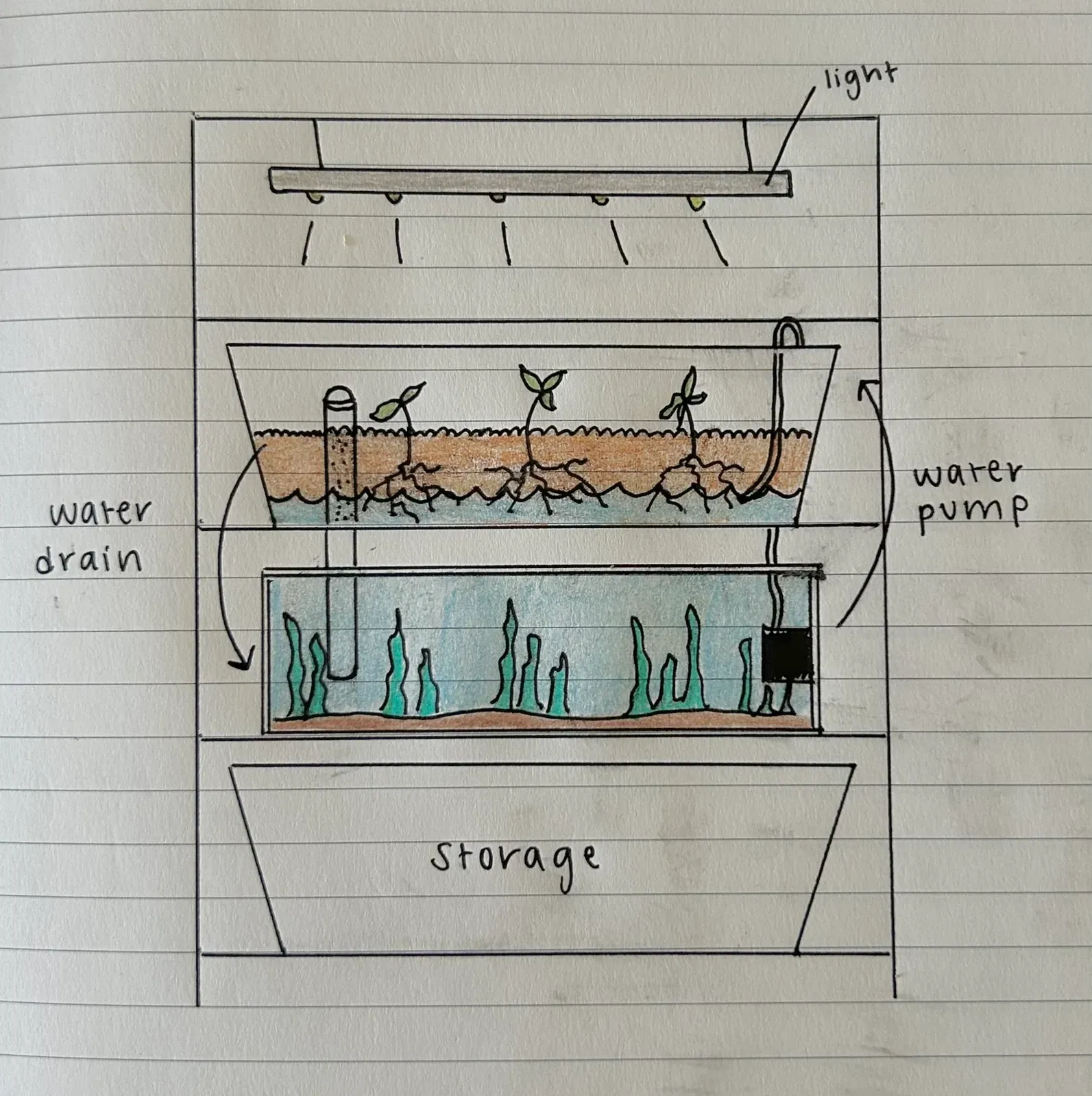
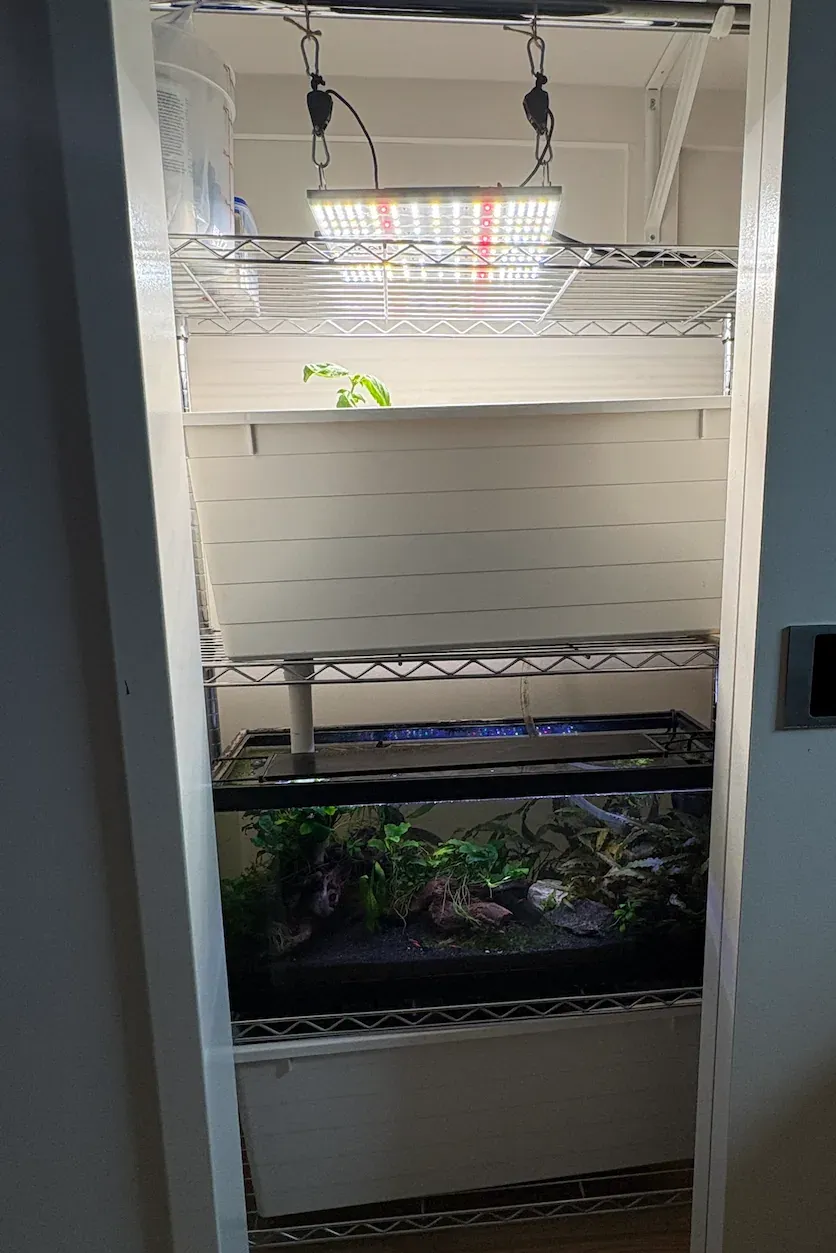
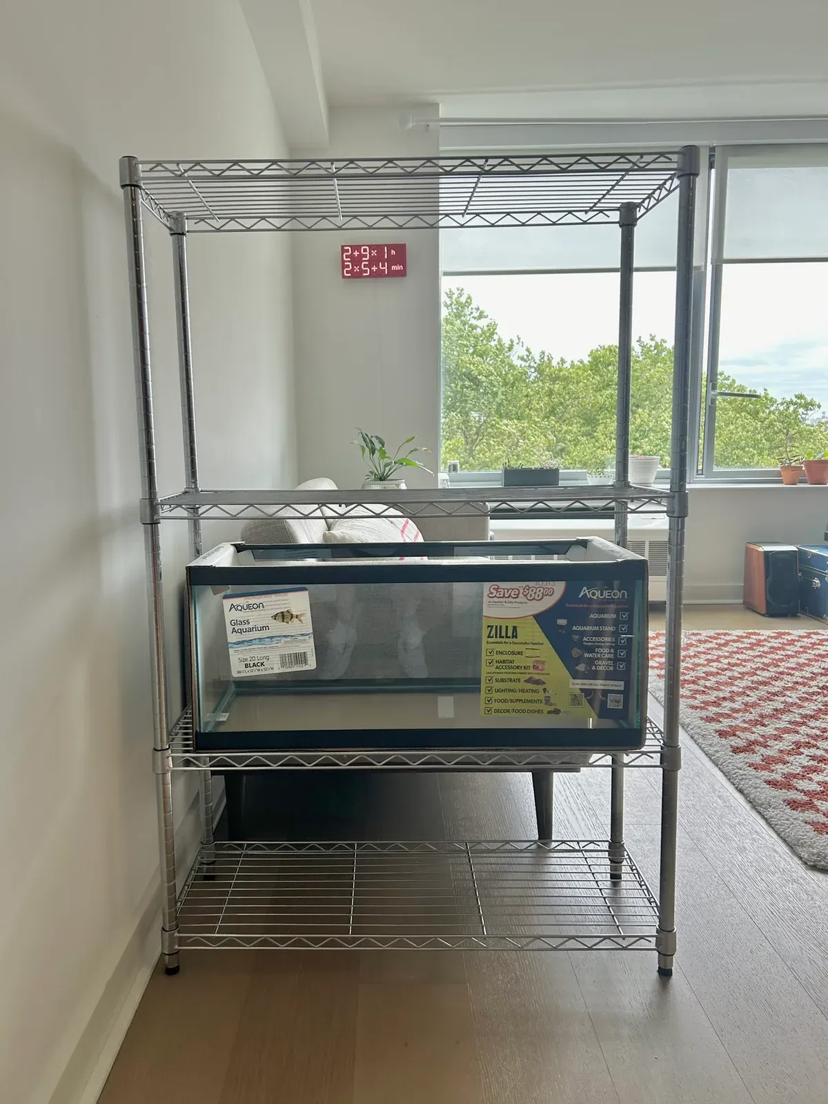
  18. NYC Apartment Aquaponics20
  19. Extinct Media Museum Tokyo21
  20. ARC-AGI Leaderboard22
  21. Firefox Containers Preview23
  22. Bitchat is now on Radicle24
  23. Show HN: Brolly, a plain-text weather forecast site24
  24. Sperm Whales blow bubbles to achieve restful, vertical sleep25
  25. Producing ammonia and fertiliser using wind power in Morris, Minnesota26
  26. Taylor Farms Called White House to Try to Delay Cyclospora Recall27
  27. Did they ghost you?27
  28. Stolen Buttons28
  29. Show HN: I made some transistor animations29
  30. Charles Ross spent 50 yrs building Star Axis naked-eye observatory in New Mexico29
The Daily Front Page 2 of 30
Saturday, July 25, 2026 The Daily Front No. #260725 — The Locked Debugger
article

Android may soon restrict on-device ADB

by shscs911·▲ 941 points·461 comments·kitsumed.github.io ↗
restricting On-Device ADB connections to protect from “bad actors”

Changes proposed for ADB could kill an entire ecosystem of open-source power-user apps, mobile developer setups, and rootless privacy tools based on Shizuku.

Early Warning

Before we dive in, please note that this is not an official Google announcement. Instead, this is based on a recent, ongoing feature request on Google IssueTracker, in which a comment by one of the core ADB maintainers (Google employee) talked about restricting On-Device ADB connections to protect from “bad actors”.

Before you stop what you are doing to head over to that IssueTracker thread, please read this carefully:

If you plan to visit the issue tracker just to post low-quality comments (such as “Hey, don’t do this, I need Shizuku!”), complaints about monopoly, or insults, I highly recommend that you refrain from doing so. Spamming the thread will only cause Google developers to lock the issue, ignore valuable community feedback, or stop sharing public updates about this change entirely.

I think a change like this could benefit Google as it goes well along their new Sideloading changes, but I do not actively believe this is what is going on here. There is a true, valid reason behind this, and I think two different approach can be taken. We will talk about it in this blog post.

How You Can Help:

  • If you have a unique use case: If you are directly affected and can write a detailed, constructive message explaining your workflow, providing links, or offering technical solutions/compromises, please, by all means, share your feedback in Google issue.
  • If your use case has already been mentioned: You do not need to repeat it. Instead, simply click the +1 button in the top right corner of the Google IssueTracker to let Google know you are affected, and toggle notifications to stay updated on the discussion.

I am hesitant to make this blog post, as I fear it may overload the few developers that work on ADB. I am unsure if I should wait more and see what happens or hold it longer and see what approach they take. Waiting too long could also be bad… As of writing this, I am unsure when/if this post will release. I saw some recent updates on assignments which were given to the main guy who previously worked on ADB, so we will see what happens.

Introduction

Hi! I’m Kitsumed, developer of ShizuCallRecorder, a Shizuku based application. As you may have guessed by now, I would be affected by this change. Obviously, I would really like it if they do not proceed with it in a way that prevent loopback connections.

To talk briefly about myself, I made ShizuCallRecorder to help with some of my own disabilities. I can get by without it, but it’s much easier with it.

You could say I have a very unique use case, and I keep discovering other unusual ones, like this person on Reddit, who used my application to preserve the voicemail of a deceased loved one.

Call recording on Android is a complicated topic. There are countless user requests, an official attempt to add the feature in Android 11 that was later canceled, and many closed-source, privacy-invasive applications that use work-arounds.

I used to hear that many users with disabilities had to trade their privacy for an easier daily life. I guess that’s what people mean when they talk about those trade-offs.

Don’t even get me started on OEMs that force an audio warning such as “This call is being recorded,” when it’s in places where it’s not legally required. People often don’t react well to that, even if you explain why you’re recording the call, it gives a bad impression. To be honest, I probably wouldn’t react well to it either.

I’m sure most of you have a more “power-user” use of Shizuku or even use loopback ADB for developer tasks. I do those too, but I wanted to point out one of my unique use case.

Alright, back on the main topic. Before I explain what the proposed change is, I’m going to explain what is ADB for less technical users.

What’s ADB?

ADB, also called Android Debug Bridge, is protocol created by Google to let developers do developer things on Android devices…

Basically, it grant us a high level of privileges, give us access to a lot of sensible commands to tests how the phone and application behave. Useful stuff for any developers or power-users.

ADB was originally designed to work over a USB connection, but later expanded how it could works:

  • USB: The original way. ADB communicates directly over a USB cable.
  • TCP/IP: Introduced as a way to run ADB over a network using an IP address and port (typically port 5555). The connection carries ADB traffic in plain text and provides a YES/NO prompt as authentication. Can only be enabled once you already have an active ADB connection.
  • Wireless Debugging (Wifi 1.0/2.0): Introduced in Android 11, it aims to improve the legacy TCP/IP workflow. It requires pairing the computer with the device using a pairing code or QR code, then establishes an authenticated and encrypted connection for subsequent ADB sessions. It does not require an active ADB connection to be enabled.

What’s a On-Device ADB connection?

ADB was originally intended to be used with two devices (simplified explanation): the Android device being debugged run the ADB Daemon (ADBD) and a separate developer machine run the ADB client. In practice, however, this setup is not always convenient. Some developers work directly from their Android device and do not have access to a second machine.

This led to usage of On-Device ADB (this is not a official term). By using a terminal emulator such as Termux, developers can run an ADB client directly on their phone and establish a connection to the local daemon (ADBD) server using either ADB TCP/IP or Wireless Debugging. Since both the client and server are running on the same device, the connection is made through the loopback address (127.0.0.1). That’s what I call On-Device ADB.

While this is a niche use case compared to how ADB intended to be used, it has led to the creation of projects such as libadb-android by MuntashirAkon and Shizuku by RikkaApps. These projects, along with many others, have created a large open-source community that made a wide range of tools for developers and power-users.

The proposed change

A new feature was made on Google IssuerTracker to allow developers to choose what interface ADBD (ADB server daemon) would listen to.

This feature was proposed following a major security issue identified as CVE-2026-0073, which allowed the Wireless ADB authentication process to be fully bypassed. What is proposed in this issue is actually a nice idea.

Right now, ADBD makes itself available on every network your phone is connected to. This feature request asks to let developers choose which interface is chosen, reducing the exposure.

The problem

The problem lies in the response from one of ADB core maintainers:

sa…@google.com:

Connection to localhost has also been the source of exploit where app are using that socket to adbd to escalate their privileges.

What about we restrict to always only binding to wifi interface wlan0 ?

Here, we can see that the employee talk about only allowing wlan0, the interface of the Wifi connection. Doing so would break many things, On-Device ADB, ADB via VPN, ADB via Ethernet, and many other unique developers setups.

Another issue I see here is the stance they seems to currently have on “On-Device ADB”. Their comment suggests that On-Device ADB is viewed primarily as an exploit bad actors can use to elevate privileges, yet there a lot of legitimate usages of on-device ADB. Developers themself uses it when they can’t access a computer.

While it can indeed be used to elevate privileges, a “malicious” application cannot do so alone. It requires multiples actions that MUST be perfomed by a human.

Why On-Device ADB Is Not Really Used by Bad Actors

A malicious application could use an on-device ADB connection to perform privilege escalation. However, it cannot establish one by itself.

To illustrate this, I’ve laid out the general limitations a bad actor would face in a few scenarios, similar to my comment on IssueTracker.

Scenario 1: General Android Users

  1. You install a malicious application.

    • ADB is disabled. ADBD is not running, and the application does not have the WRITE_SECURE_SETTINGS permission, as it must be manually granted via ADB. No exploitation attempts are possible.

Scenario 2: A Developer on Android 11+ Using Wireless ADB

  1. You install a malicious application.
  2. You enable USB debugging, starting ADBD.
  3. You enable Wireless ADB. ADBD is now running on your phone and listening on all network interfaces.
  4. The application would need to perform the one-time pairing process. This requires the user to manually retrieve the one-time code from Settings and provide it. No exploitation attempts are possible.

Scenario 3: A Developer Using ADB over TCP/IP

  1. You install a malicious application.
  2. You enable USB debugging, starting ADBD.
  3. You connect via USB ADB to enable TCP/IP, then disconnect the USB cable.
  4. ADBD continues running and listens on all network interfaces.
  5. The application initiates a connection, causing an authorization prompt to appear on the screen. If the user selects No, the connection is rejected. No silent exploitation attempts are possible.

Conclusion

In a normal scenario, a bad actor cannot gain an ADB connection. It is only possible while the developer is actively using ADB on the device, because a bad actor cannot start ADBD by themselves.

However, if we return to a scenario such as CVE-2026-0073, exploitation would become possible in Scenarios 2 and 3, but only after the user has manually enabled USB debugging. As for scenario 3, it would also require the developer to MANUALLY enable TCP/IP. I can understand the motivation for preventing loopback connections by default, but not to fully prevents it.

There is a difference between preventing it by default and permanently preventing it. I think this should be something users can disable through a persistent setting. By this, I mean a toggle that survives a reboot (else it would make tools like Shizuku impracticals) and, ideally, cannot be read by third-party applications. Otherwise, developers would have to repeatedly disable it whenever banking apps or games detect that on-device ADB is availabl. That said, this part could be worked around once a application is manually granted WRITE_SECURE_SETTINGS.

I think that justifying blocking it because a human could perform actions to allow it would be far-fetched. A human could also designate a malicious application as a device administrator or grant it Accessibility permissions, and yet we would not get rid of those features.

I believe it should be an assumed risk that disabling such a security feature enables on-device debugging while also exposing the device to the rare possibility of a future vulnerability. To me, the feature/risk ratio make sense here, as there is a real, legitimate usage.

Although it may have not been originally intended, On-Device ADB has enabled a niche ecosystem of developer and power-user tools, including projects such as App Manager, libadb-android, Canta, aShell, ShizuWall, ShizuCallRecorder and Shizuku.

To conclude, I would like to mention my conclusion in What Is Shizuku? How Does It Work? Security Implications?, where I said as a joke:

Here’s my closing thought: I can’t wait to see how they’ll justify disabling loopback ADB over TCP/IP connections on non-emulator devices and start requiring a Google account…

Well I guess they may indeed disable loopback ADB. Huh… I was almost 100% right on that one I guess. If you are a technical user, I invite you to give your feedback inside the issue here. Please don’t forget the early warning.

The Daily Front Page 3 of 30
Saturday, July 25, 2026 The Daily Front No. #260725 — The Model Horse Race
article

Opus 5 is currently #1 on Artificial Analysis Intelligence Leaderboard

by aarondong·▲ 366 points·223 comments·artificialanalysis.ai ↗
Claude Opus 5 (max) and Claude Opus 5 (xhigh) are the highest intelligence models.

Microevals Playground

Comparison and analysis of AI models across key performance metrics including quality, price, output speed, latency, context window & others. Click on any model to see detailed metrics. For more details including relating to our methodology, see our FAQs.

Intelligence

Claude Opus 5 (max) logo Claude Opus 5 (max) and Claude Opus 5 (xhigh) logo Claude Opus 5 (xhigh) are the highest intelligence models, followed by Claude Fable 5 (with fallback) logo Claude Fable 5 (with fallback) and GPT-5.6 Sol (max) logo GPT-5.6 Sol (max).

Output Speed (tokens/s)

Mercury 2 logo Mercury 2 (902 t/s) and HyperNova 60B 2605 logo HyperNova 60B 2605 (414 t/s) are the fastest models, followed by Granite 4.0 H Small logo Granite 4.0 H Small and Gemini 3.5 Flash-Lite logo Gemini 3.5 Flash-Lite.
Latency (seconds)

Gemini 2.5 Flash-Lite logo Gemini 2.5 Flash-Lite (0.35s) and Command A+ logo Command A+ (0.42s) are the lowest latency models, followed by Gemini 2.5 Flash logo Gemini 2.5 Flash and North Mini Code logo North Mini Code.

Price ($ per M tokens)

Devstral 2 logo Devstral 2 ($0.00) and North Mini Code logo North Mini Code ($0.00) are the cheapest models, followed by Gemma 3 4B logo Gemma 3 4B and Gemma 3 27B logo Gemma 3 27B.

Context Window

Llama 4 Scout logo Llama 4 Scout (10M) and Grok 4.20 0309 logo Grok 4.20 0309 (2M) are the largest context window models, followed by Gemini 1.5 Pro (May) logo Gemini 1.5 Pro (May) and Grok 4.1 Fast logo Grok 4.1 Fast.

Intelligence

Artificial Analysis Intelligence IndexCoding IndexAgentic Index

Artificial Analysis Intelligence Index

Artificial Analysis Intelligence Index v4.1 incorporates 9 evaluations: GDPval-AA v2, 𝜏³-Banking, Terminal-Bench v2.1, SciCode, Humanity's Last Exam, GPQA Diamond, CritPt, AA-Omniscience, AA-LCR

27 of 586 models

Add model from specific provider

Reasoning models are indicated by a lightbulb icon

Artificial Analysis Intelligence Index

Artificial Analysis Intelligence Index v4.1 includes: GDPval-AA v2, 𝜏³-Banking, Terminal-Bench v2.1, SciCode, Humanity's Last Exam, GPQA Diamond, CritPt, AA-Omniscience, AA-LCR. See Intelligence Index methodology for further details, including a breakdown of each evaluation and how we run them.

Open Weights / ProprietaryReasoning / Non-ReasoningText Only / Multimodal Inputs

Artificial Analysis Intelligence Index by Open Weights / Proprietary

Artificial Analysis Intelligence Index v4.1 incorporates 9 evaluations: GDPval-AA v2, 𝜏³-Banking, Terminal-Bench v2.1, SciCode, Humanity's Last Exam, GPQA Diamond, CritPt, AA-Omniscience, AA-LCR

27 of 586 models

Add model from specific provider

ProprietaryOpen WeightsOpen Weights (Commercial Use Restricted)

Reasoning models are indicated by a lightbulb icon

Artificial Analysis Intelligence Index

Artificial Analysis Intelligence Index v4.1 includes: GDPval-AA v2, 𝜏³-Banking, Terminal-Bench v2.1, SciCode, Humanity's Last Exam, GPQA Diamond, CritPt, AA-Omniscience, AA-LCR. See Intelligence Index methodology for further details, including a breakdown of each evaluation and how we run them.

Open Weights

Indicates whether the model weights are available. Models are labelled as 'Commercial Use Restricted' if the weights are available but commercial use is limited (typically requires obtaining a paid license).

Intelligence Breakdown

Intelligence Evaluations

Intelligence evaluations measured independently by Artificial Analysis · Higher is better

18 of 22 evaluations

27 of 586 models

Add model from specific provider

GDPval-AA v2

Agentic real-world work tasks, (Elo-500)/2000

𝜏³-Banking

Agentic tool use

Terminal-Bench v2.1

Agentic coding & terminal use

SciCode

Coding

Humanity's Last Exam

Reasoning & knowledge

GPQA Diamond

Scientific reasoning

CritPt

Physics reasoning

AA-Omniscience Accuracy

Knowledge

AA-Omniscience Non-Hallucination Rate

1 - hallucination rate

AA-LCR

Long context reasoning

AA-Briefcase

Agentic knowledge work, Elo

AutomationBench-AA

Agentic SaaS workflows

Harvey LAB-AA

Legal agentic work, criterion pass rate

EnterpriseOps-Gym-AANew

Agentic business operations

IFBench

Instruction following

APEX-Agents-AA

Long-horizon agentic tasks

ITBench-AA

Kubernetes incident root-cause analysis

MMMU-Pro

Visual reasoning

Reasoning models are indicated by a lightbulb icon

Intelligence Evaluation Relevance

While model intelligence generally translates across use cases, specific evaluations may be more relevant for certain use cases.

Artificial Analysis Intelligence Index

Artificial Analysis Intelligence Index v4.1 includes: GDPval-AA v2, 𝜏³-Banking, Terminal-Bench v2.1, SciCode, Humanity's Last Exam, GPQA Diamond, CritPt, AA-Omniscience, AA-LCR. See Intelligence Index methodology for further details, including a breakdown of each evaluation and how we run them.

AA-Briefcase

AA-Briefcase EloAA-Briefcase Rubric Score (%)Analytical Quality & Presentation Elo

AA-Briefcase Elo

AA-Briefcase is an agentic knowledge work benchmark developed by Artificial Analysis. AA-Briefcase Elo is a combined metric that aggregates rubric pass rate, analytical quality Elo and presentation Elo · Higher is better

24 of 56 models

Add model from specific provider

Reasoning models are indicated by a lightbulb icon

AA-Briefcase Elo

AA-Briefcase Elo is a combined metric that aggregates analytical quality Elo, presentation Elo, and rubric pass rate, with rubric performance converted into Elo via synthetic head-to-head matches. Elo and 95% confidence interval bounds are clamped at 0.

AA-Omniscience

AA-Omniscience IndexAA-Omniscience AccuracyAA-Omniscience Hallucination Rate

AA-Omniscience Index

AA-Omniscience Index (higher is better) measures knowledge reliability and hallucination. It rewards correct answers, penalizes hallucinations, and has no penalty for refusing to answer. Scores range from -100 to 100, where 0 means as many correct as incorrect answers, and negative scores mean more incorrect than correct.

26 of 456 models

Add model from specific provider

Reasoning models are indicated by a lightbulb icon

AA-Omniscience Index

AA-Omniscience Index (higher is better) measures knowledge reliability and hallucination. It rewards correct answers, penalizes hallucinations, and has no penalty for refusing to answer. Scores range from -100 to 100, where 0 means as many correct as incorrect answers, and negative scores mean more incorrect than correct.

Openness

Openness IndexOpenness Index ComponentsOpenness vs. Intelligence

Artificial Analysis Openness Index: Score

Openness Index assesses model openness on a 0 to 100 normalized scale (higher is more open)

12 of 291 models

Add model from specific provider

Reasoning models are indicated by a lightbulb icon

Intelligence Index Comparisons

Intelligence Index vs. Cost per TaskIntelligence Index vs. Time per TaskIntelligence Index vs. Output SpeedIntelligence Index vs. End-to-End Response Time

Intelligence Index vs. Cost per Intelligence Index Task

Artificial Analysis Intelligence Index · Weighted average cost (USD) per Artificial Analysis Intelligence Index task

27 of 586 models

Most attractive quadrant

XiaomiGoogleAnthropicMiniMaxOpenAINVIDIAAlibabaSpaceXAIDeepSeekMetaMistralZ AIKimi

Reasoning models are indicated by a lightbulb icon

Cost per Intelligence Index Task

Weighted average cost per Intelligence Index task. Each evaluation’s cost is calculated from input, cache hit, cache write, reasoning, and answer token prices, divided by task count, and weighted by its Intelligence Index weight.

Artificial Analysis Intelligence Index

Artificial Analysis Intelligence Index v4.1 includes: GDPval-AA v2, 𝜏³-Banking, Terminal-Bench v2.1, SciCode, Humanity's Last Exam, GPQA Diamond, CritPt, AA-Omniscience, AA-LCR. See Intelligence Index methodology for further details, including a breakdown of each evaluation and how we run them.

Token Use

Output Tokens per TaskIntelligence Index vs. Output Tokens per TaskIntelligence Index Token UseIntelligence Index vs. Token Use

Output Tokens per Intelligence Index Task

Weighted average number of output tokens used to run one task in the Artificial Analysis Intelligence Index

27 of 586 models

AnswerReasoning

Reasoning models are indicated by a lightbulb icon

Output Tokens per Intelligence Index Task

The number of tokens required per Intelligence Index task. This is calculated by multiplying the output tokens per eval by the relative weights of each benchmark in the Intelligence Index, then dividing by task count (excluding repeats).

Price and Cost

Cost per TaskIntelligence Index vs. Cost per TaskEvaluation Breakdown

Cost per Intelligence Index Task

Weighted average cost (USD) per Artificial Analysis Intelligence Index task, segmented by token type. Lower is better

27 of 586 models

AnswerReasoningCache WriteCache HitInput

Reasoning models are indicated by a lightbulb icon

Cost per Intelligence Index Task

Weighted average cost per Intelligence Index task. Each evaluation’s cost is calculated from input, cache hit, cache write, reasoning, and answer token prices, divided by task count, and weighted by its Intelligence Index weight.

Intelligence Index Total CostIntelligence Index vs. Total Cost

Cost to Run Artificial Analysis Intelligence Index

Cost (USD) to run all evaluations in the Artificial Analysis Intelligence Index

27 of 586 models

Add model from specific provider

OutputReasoningCache WriteCache ReadNon-Cache Input

Reasoning models are indicated by a lightbulb icon

Cost to Run Artificial Analysis Intelligence Index

The cost to run the evaluations in the Artificial Analysis Intelligence Index, calculated using the model's input, cache hit, cache write, reasoning, and answer token prices and the number of tokens used across evaluations (excluding repeats).

Cache Hit, Input, and Output PricingBlended PriceBlended Price (Stacked)Cache DiscountIntelligence Index vs. PriceIntelligence Index vs. Price (Log, Inverted)Image Input Pricing

Pricing: Cache Hit, Input, and Output

Price (USD per M Tokens)

27 of 586 models

Add model from specific provider

Cache HitInputOutput

Reasoning models are indicated by a lightbulb icon

Cache Hit

Price per token for cached prompts (previously processed), typically offering a significant discount compared to regular input price, represented as USD per million tokens. The values shown here are the cache hit price; cache write and cache storage are billed separately and vary by provider — see "Cache pricing by provider" for detail.

Input Price

Price per token included in the request/message sent to the API, represented as USD per million Tokens.

Cache Pricing by Provider

The blended cache price shown here uses cache hit price only. Other caching costs differ by provider:

  • Anthropic: charges a separate cache write fee, with different rates for 5-minute and 1-hour TTLs (1-hour TTL is more expensive).
  • Google (Vertex/Gemini): charges a per-hour cache storage fee in addition to cache hit pricing. Some providers also use tiered pricing for prompts above 200K tokens.
  • OpenAI, DeepSeek, others: typically charge only cache hit pricing with no write or storage fee.

See Prompt Caching for the full breakdown.

Output Price

Price per token generated by the model (received from the API), represented as USD per million Tokens.

Model Performance Representation

Figures represent performance of the model's first-party API (e.g. OpenAI for o1) or the median across providers where a first-party API is not available (e.g. Meta's Llama models).

Context Window

Context WindowIntelligence Index vs. Context Window

Context Window

Context window: tokens limit · Higher is better

27 of 586 models

Add model from specific provider

Reasoning models are indicated by a lightbulb icon

Context Window for RAG

Larger context windows are relevant to RAG (Retrieval Augmented Generation) LLM workflows which typically involve reasoning and information retrieval of large amounts of data.

Context Window

Maximum number of combined input & output tokens. Output tokens commonly have a significantly lower limit (varied by model).

Speed

Measured by Output Speed (tokens per second)

Output SpeedOutput Speed by Prompt TypeOutput Speed VarianceOutput Speed Over TimeOutput Speed vs. PriceLatency vs. Output Speed

Output Speed

Output tokens per second · Higher is better

27 of 586 models

Add model from specific provider

Reasoning models are indicated by a lightbulb icon

Output Speed

Tokens per second received while the model is generating tokens (ie. after first chunk has been received from the API for models which support streaming).

Model Performance Representation

Figures represent performance of the model's first-party API (e.g. OpenAI for o1) or the median across providers where a first-party API is not available (e.g. Meta's Llama models).

Time per TaskIntelligence Index vs. Time per TaskCost vs. Time per Task

Time per Intelligence Index Task

Weighted average decode time (minutes) per task; excludes TTFT and overhead time · Lower is better

27 of 586 models

Reasoning models are indicated by a lightbulb icon

Time per Intelligence Index Task

The weighted average time (seconds) per Artificial Analysis Intelligence Index task. This is calculated by dividing output tokens per task by output speed, weighted by the relative weights of each benchmark in the Intelligence Index.

Latency

Measured by Time (seconds) to First Token

Time To First Answer TokenTime To First TokenLatency by Prompt TypeLatency VarianceLatency Over Time

Latency: Time To First Answer Token

Seconds to first answer token received · Accounts for reasoning model 'thinking' time

27 of 586 models

Add model from specific provider

Thinking (reasoning models, when applicable)Input processing

Reasoning models are indicated by a lightbulb icon

Time to First Answer Token

Time to first answer token received, in seconds, after API request sent. For reasoning models, this includes the 'thinking' time of the model before providing an answer. For models which do not support streaming, this represents time to receive the completion.

End-to-End Response Time

Seconds to output 500 tokens, calculated based on time to first token, 'thinking' time for reasoning models, and output speed

End-to-End Response TimeEnd-to-End Response Time by Prompt TypeEnd-to-End Response Time Over Time

End-to-End Response Time

Seconds to output 500 tokens, including reasoning model 'thinking' time · Lower is better

27 of 586 models

Add model from specific provider

Outputting time'Thinking' time (reasoning models)Input processing time

Reasoning models are indicated by a lightbulb icon

End-to-End Response Time

Seconds to receive a 500 token response. Key components:

  • Input time: Time to receive the first response token
  • Thinking time (only for reasoning models): Time reasoning models spend outputting tokens to reason prior to providing an answer. Amount of tokens based on the average reasoning tokens across a diverse set of 60 prompts (methodology details).
  • Answer time: Time to generate 500 output tokens, based on output speed

Model Performance Representation

Figures represent performance of the model's first-party API (e.g. OpenAI for o1) or the median across providers where a first-party API is not available (e.g. Meta's Llama models).

Model Size (Open Weights Models Only)

Total & Active ParametersIntelligence Index vs. Active ParametersIntelligence Index vs. Total Parameters

Model Size: Total and Active Parameters

Comparison between total model parameters and parameters active during inference

27 of 586 models

Add model from specific provider

Active ParametersPassive Parameters

Reasoning models are indicated by a lightbulb icon

Total Parameters

The total number of trainable weights and biases in the model, expressed in billions. These parameters are learned during training and determine the model's ability to process and generate responses.

Active Parameters at Inference Time

The number of parameters actually executed during each inference forward pass, expressed in billions. For Mixture of Experts (MoE) models, a routing mechanism selects a subset of experts per token, resulting in fewer active than total parameters. Dense models use all parameters, so active equals total.

Frequently Asked Questions

Which is the most intelligent AI model?

Claude Opus 5 (Adaptive Reasoning, Max Effort) currently leads the Artificial Analysis Intelligence Index with a score of 61, out of 170 models evaluated.

What are the top AI models?

The top AI models by Intelligence Index are: 1. Claude Opus 5 (Adaptive Reasoning, Max Effort) (61), 2. Claude Opus 5 (Adaptive Reasoning, Xhigh Effort) (60), 3. Claude Fable 5 (Adaptive Reasoning, Max Effort, Opus 4.8 Fallback) (60), 4. GPT-5.6 Sol (max) (59), and 5. Claude Opus 5 (Adaptive Reasoning, High Effort) (59).

Which is the fastest AI model?

Mercury 2 is the fastest at 901.6 tokens per second, followed by HyperNova 60B 2605 (414.2 t/s) and Granite 4.0 H Small (407.1 t/s).

Which is the cheapest AI model?

Nova Micro is the most affordable at $0.03 per 1M tokens (blended), followed by Sarvam 30B (high) ($0.03) and Gemma 4 E4B (Non-reasoning) ($0.03).

Which AI model has the lowest latency?

Gemini 2.5 Flash-Lite (Non-reasoning) has the lowest time to first token at 0.35s, followed by Command A+ (0.42s) and Gemini 2.5 Flash (Non-reasoning) (0.49s).

Which is the best open weights AI model?

GLM-5.2 (max) is the highest-ranked open weights model with an Intelligence Index score of 51. There are 94 open weights models out of 170 total evaluated.

What are the top open weights AI models?

The top open weights AI models by Intelligence Index are: 1. GLM-5.2 (max) (51), 2. MiniMax-M3 (44), and 3. DeepSeek V4 Pro (Reasoning, Max Effort) (44).

Which is the best reasoning model?

Claude Opus 5 (Adaptive Reasoning, Max Effort) leads among 126 reasoning models with an Intelligence Index score of 61. Reasoning models use extended thinking to work through complex problems before providing answers.

How are AI models compared on Artificial Analysis?

Models are compared across multiple dimensions including intelligence (quality), pricing, output speed (tokens per second), latency (time to first token), end-to-end response time, and context window size. Performance metrics are measured directly using standardized prompts across 586 models.

How do I compare a specific model against others?

Click on any model name or row in the charts to view its dedicated page with detailed metrics and direct comparisons against similar models. You can also use the model selector to customize which models appear in each chart. View the leaderboard

The Daily Front Page 4 of 30
Saturday, July 25, 2026 The Daily Front No. #260725 — Open Weights at the Crossroads
article

Open-weight AI is having its Kubernetes moment

by tknaup·▲ 381 points·296 comments·tobi.knaup.me ↗
Open-weight models are becoming the foundation for the next AI ecosystem.

Open-weight AI is having its Kubernetes moment. Let's not ruin it.

Open-weight models are becoming the foundation for the next AI ecosystem. The US should compete in it, not wall itself off.

I have seen a version of this story before.

In 2013 I co-founded Mesosphere, an open source cloud-native software company. We built on Apache Mesos, which my co-founder Ben Hindman had helped create at UC Berkeley. We later built DC/OS (Data Center Operating System) around Mesos, released it as open source, and commercialized it through an enterprise distribution with support and proprietary features.

After several years of massive growth, Kubernetes disrupted us. It was newer, fully open source, and it quickly galvanized the cloud-native community. Many of the world’s best distributed-systems and infrastructure engineers bet their careers on it, and even some of our most loyal community members changed horses.

Once that happened, innovation moved to Kubernetes. Whatever the platform was missing, someone started building: networking, storage, observability, deployment tools, policy engines. A large number of startups were created, and legacy vendors joined in as well. Almost every component required to run Kubernetes in production became available as open source. Cloud providers and companies including Mesosphere/D2iQ, Rancher, Red Hat and Nutanix then built businesses around integration, enterprise features, support and operations.

Kubernetes did not win simply because its repository was public. It became a neutral substrate that engineers, cloud providers and enterprise vendors could all extend to fit their customers’ needs. Common interfaces and vendor-neutral governance gave everyone confidence that they could build on it.

The lesson I took away wasn’t that open source always wins. It was that once an open platform that people can customize becomes the industry’s center of gravity, no single vendor can match the combined rate of innovation around it.

I think AI is approaching the same point.

Open weights turn a model into a platform

First, a terminology note. Most models we casually call “open source” are more accurately described as open-weight. You can download and modify the trained parameters, but the training data and complete training process usually aren’t available. That falls short of the Open Source Initiative’s definition of open source AI. The distinction matters. It doesn’t, however, prevent an ecosystem from forming around the artifact people can run and modify.

The Kubernetes analogy isn’t perfect. Kubernetes contributors could inspect and change the actual source, and improvements could flow back into a shared upstream project. Model fine-tunes usually don’t work that way. Frontier weights may be downloadable but still require expensive hardware, and there is no AI equivalent of the CNCF providing neutral governance and common interfaces. Those are real differences. The common mechanism is that a sufficiently capable, portable substrate can attract complementary innovation far beyond what its original creator could build alone.

The first reason to use open-weight models was self-hosting. Companies wanted control over their data. They wanted to run models in their own cloud or data center. And as usage and inference costs grow, they increasingly want control over cost as well.

That demand produced a healthy open source serving stack: vLLM, SGLang, llama.cpp, Ollama, MLX and others.

But self-hosting is only the beginning. Open weights turn the model itself into something developers can adapt and redistribute. Hugging Face now hosts more than two million public models. Around popular families such as Qwen and Gemma, developers produce:

  • quantized and converted weights for different silicon architectures and scale;
  • fine-tunes and LoRA adapters for coding, medicine, law, math and agentic workflows;
  • model merges that combine different fine-tunes;
  • adaptations for runtimes such as TensorRT-LLM, vLLM, MLX and others.

Until recently, it was easy to dismiss this activity at the frontier. Open models were useful, but the base models weren’t good enough for the hardest coding and agentic tasks. That gap is narrowing quickly. Z.ai has released GLM-5.2 with public weights under an MIT license. Its own evaluation reports 62.1% on SWE-bench Pro versus 58.6% for GPT-5.5, although results vary across benchmarks and agent harnesses.

Moonshot says Kimi K3 approaches the closed frontier on long-horizon coding and has promised to publish its weights on July 27. Artificial Analysis supports the performance claim, scoring it alongside Opus 4.8 and GPT-5.5 in its independent evaluation.

Once the base model is good enough, the ecosystem can compound. I expect new projects around agent runtimes, coding harnesses, sandboxes, evaluations, observability and specialized fine-tunes. Together they can become a production-grade stack: an open-weight model running on open source software, customizable for a team’s workload, hardware and economics.

Will that stack beat every closed model on every benchmark? Probably not. But I would not bet on any single vendor out-innovating the combined open ecosystem over time. Frontier technology is a talent war, and open ecosystems give talented people everywhere a reason to build on the same foundation.

Banning Chinese models would be an own goal

This brings us to the current debate in Washington. After the release of Kimi K3 and other capable Chinese models, the Trump administration is reportedly considering restrictions on Chinese open-weight models. The exact form of a potential ban remains unclear.

A broad ban on American researchers and companies using Chinese open-weight models would do something else entirely. It would cut the US off from an ecosystem that is already attracting many of the world’s best AI researchers and engineers, including a large number of Chinese researchers. The rest of the world would keep building. American developers would be the ones locked out.

We’ve seen this dynamic with Qwen already. Hugging Face reports that Chinese models accounted for 41% of model downloads over the past year. If the best open-weight foundation models increasingly come from China, innovation will accumulate around them in the same way it accumulated around Kubernetes.

How the US should compete

The US should compete in that ecosystem, not retreat from it.

Release frontier-grade American models

American labs need to release frontier-grade open-weight models under licenses that startups can actually build on. There has been progress. NVIDIA’s Nemotron models are commercially usable under NVIDIA’s own permissive license. Thinking Machines released Inkling under Apache 2.0, as did OpenAI with gpt-oss and Google with Gemma 4. But OpenAI’s and Google’s strongest models remain closed, as do those from most American frontier labs.

Use procurement to create an open market

The government should use procurement to create demand for portable, interoperable systems rather than permanent dependence on one API vendor. The Department of Defense has done this before. Platform One provides open source tools and enterprise products that different military programs can build on. The same playbook can accelerate innovation around open-weight models.

Build the rest of the stack

American companies need to build the rest of the stack. Startups can customize and extend the models, embed them into products, and provide the serving, tooling, support and operational layers. Our leading silicon companies will keep improving the hardware. Hyperscalers and neoclouds can serve the models and their ecosystems.

Set standards instead of banning models

Safety is the strongest argument for restrictions, but a blanket ban is too blunt and would sacrifice access to the entire ecosystem. A better approach is independent testing and standards for frontier models. The analogy isn’t exact: Kubernetes conformance tests compatibility, not safety. But the governance model is useful. Demis Hassabis has proposed a US-led independent standards body along those lines.

America should not respond to open Chinese models by building a wall around its own developers. We should run the models ourselves, tear them apart, benchmark them, improve on them and build better American alternatives. Then we should make the American stack the easiest one in the world to adopt.

The United States has spent decades attracting the world’s best technical talent and giving it room to build. Turning that advantage into a walled garden while the rest of the world standardizes on a more open stack would be a spectacular own goal. We would be giving up our role as the AI leader by choice.

The Daily Front Page 5 of 30
Saturday, July 25, 2026 The Daily Front No. #260725 — Prompt Diet
article

The new rules of context engineering for Claude 5 generation models

by mellosouls·▲ 358 points·257 comments·claude.com ↗
We removed over 80% of Claude Code's system prompt for more advanced models.

We removed over 80% of Claude Code's system prompt for more advanced models. How to apply the lessons we learned to your own context engineering in Claude Code and with your own agents.

I’ve written previously about how to best prompt the newest generation of Claude 5 models and work with them iteratively to discover what you want to build.

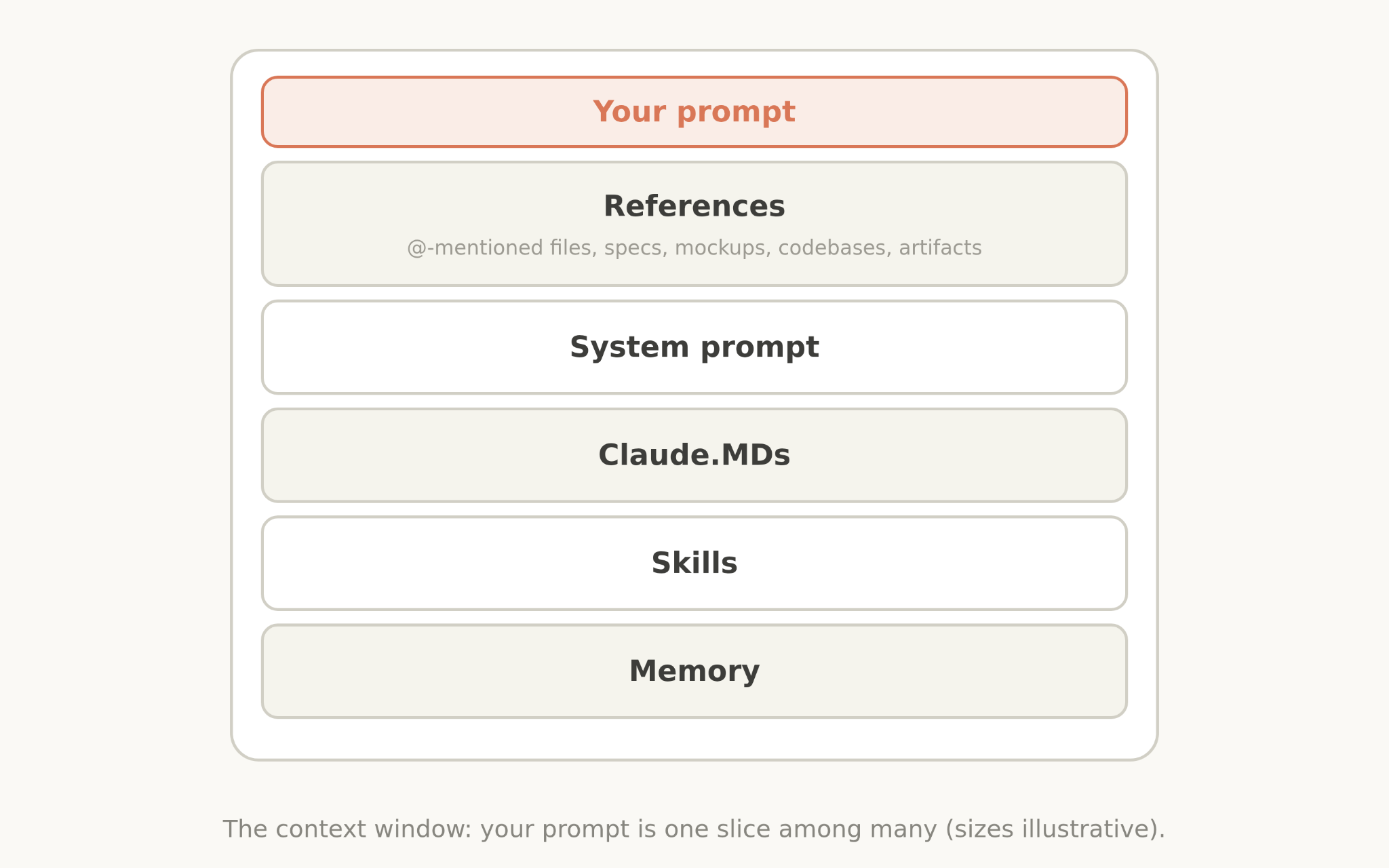
But when you send a message to Claude, the prompt is only a small part of the context it gets. Much of your context is assembled from your system prompt, Skills, CLAUDE.md files, memory, and other sources. We call this context engineering, and it makes a big impact on the results you generate when using Claude Code or in building your own agents.

Unlike a prompt, context is used generally across many requests, so it cannot be as specific.  How do you build these general prompts and guidance for Claude, especially when you don’t know what a user’s prompt might be?

This can be surprisingly difficult as Claude’s own capabilities evolve. Most recently, we noticed a large jump in the way we prompt the newest generation of Claude models. We removed over 80% of Claude Code’s system prompt for models like Claude Opus 5 and Claude Fable 5 with no measurable loss on our coding evaluations.

Here’s what we’ve learned about prompting this new class of models, and how you can utilize it to update your context engineering. We’ve put these best practices in claude doctor; use the command /doctor in Claude Code to rightsize your skills, and CLAUDE.md files.

Unhobbling Claude

Overall, we found that we were overconstraining Claude Code, both through our system prompt and in our CLAUDE.md files and skills. 

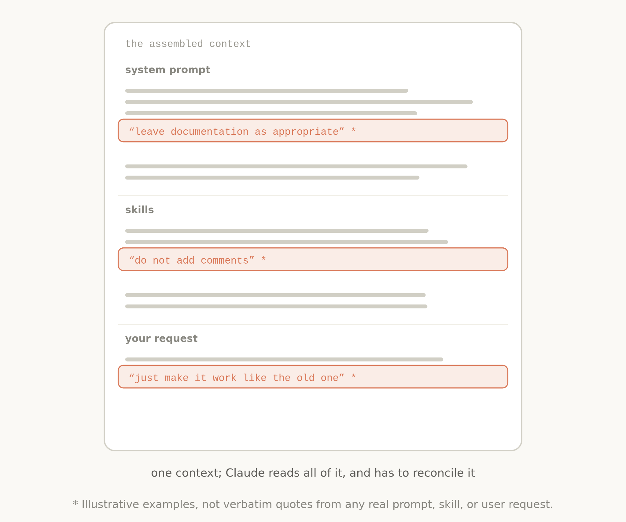
For example, when we read transcripts of our own internal usage of Claude Code, we see several conflicting messages in a single request like “leave documentation as appropriate,” or “DO NOT add comments” as our system prompt, skills, and user requests clash with each other. 

Generally, Claude can interpret the user’s intent to get to the right answer, but Claude must think more carefully about these overlapping and conflicting messages before deciding what to do.

And while these constraints were once needed to avoid worst case scenarios, we have since found we can delete many of them and let the model use surrounding context and judgement instead.

Additionally, Claude Code now has many more tools. Claude used to rely on CLAUDE.md as a source of memory, information, and guidance. Now we have memory, artifacts, and skills, which Claude can use to create new ways of loading and sharing context across sessions.

Then and now

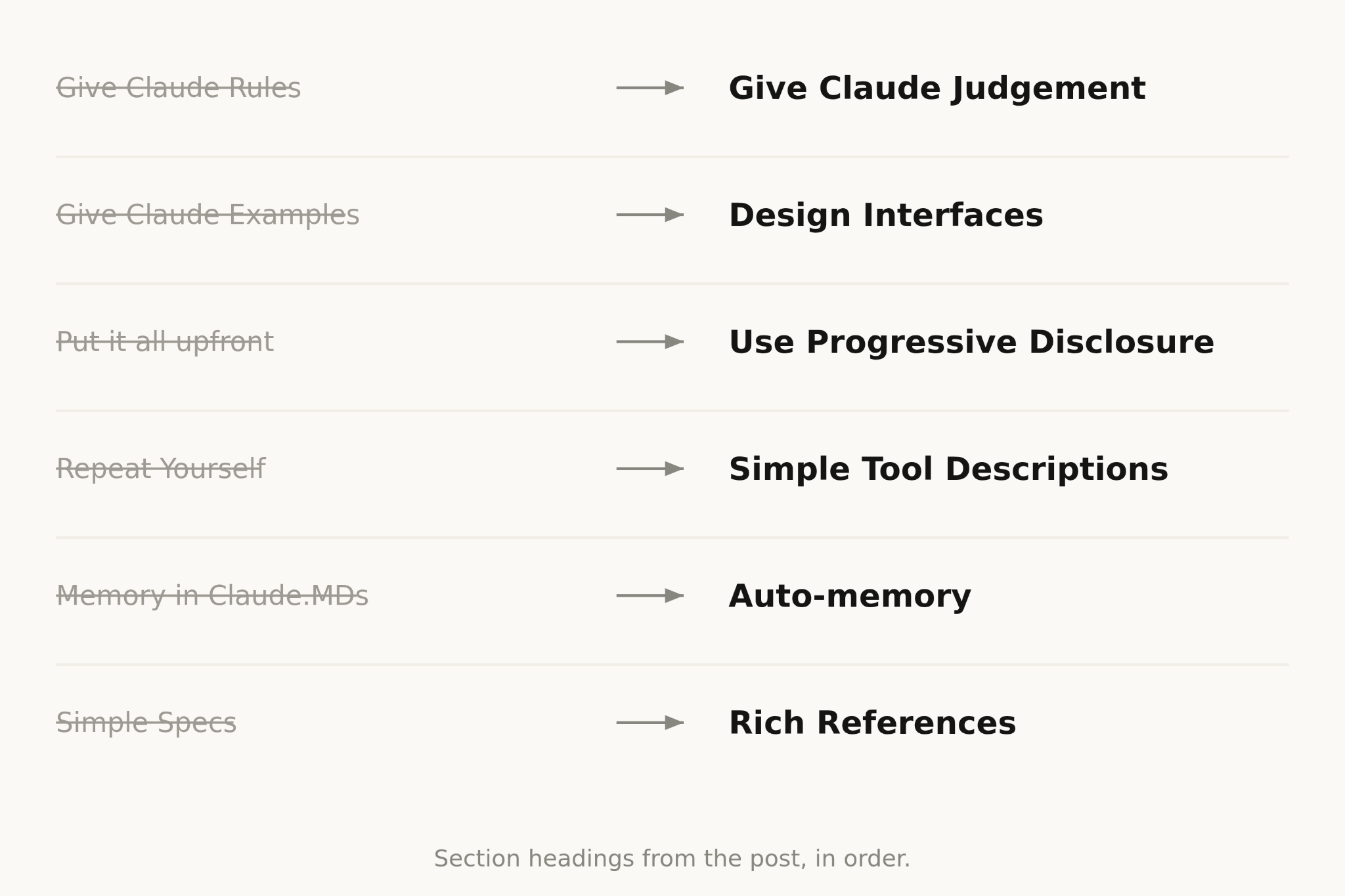
There were a number of previous context engineering best practices that had become myths. Including:.

Then: Give Claude rules

Now: Let Claude use judgement

When we first rolled out Claude Code, we needed to be sure that Claude avoided worst case scenarios, such as deleting files. This meant we would give particularly strong guidance that might not always be true, For example, in the system prompt we used to say: 

In code: default to writing no comments. Never write multi-paragraph docstrings or multi-line comment blocks — one short line max. Don't create planning, decision, or analysis documents unless the user asks for them — work from conversation context, not intermediate files.

But for a certain subset of prompts, this guidance would be wrong. In the case of documentation, the user may have their own preferences, or specific parts of very complex code might need multi-line comment blocks.

Still, without these guardrails for older models, the comments Claude wrote would be incorrect in many cases and we had to accept this tradeoff. But newer models have better judgement and can handle these decisions well without explicit rules. 

In the new system prompt we say: Write code that reads like the surrounding code: match its comment density, naming, and idiom.

Then: Give Claude examples

Now: Design interfaces

The number one rule for tool usage was to give Claude examples on how to use them. With our newest models, we’ve found that giving examples actually constrains them to a certain exploration space. 

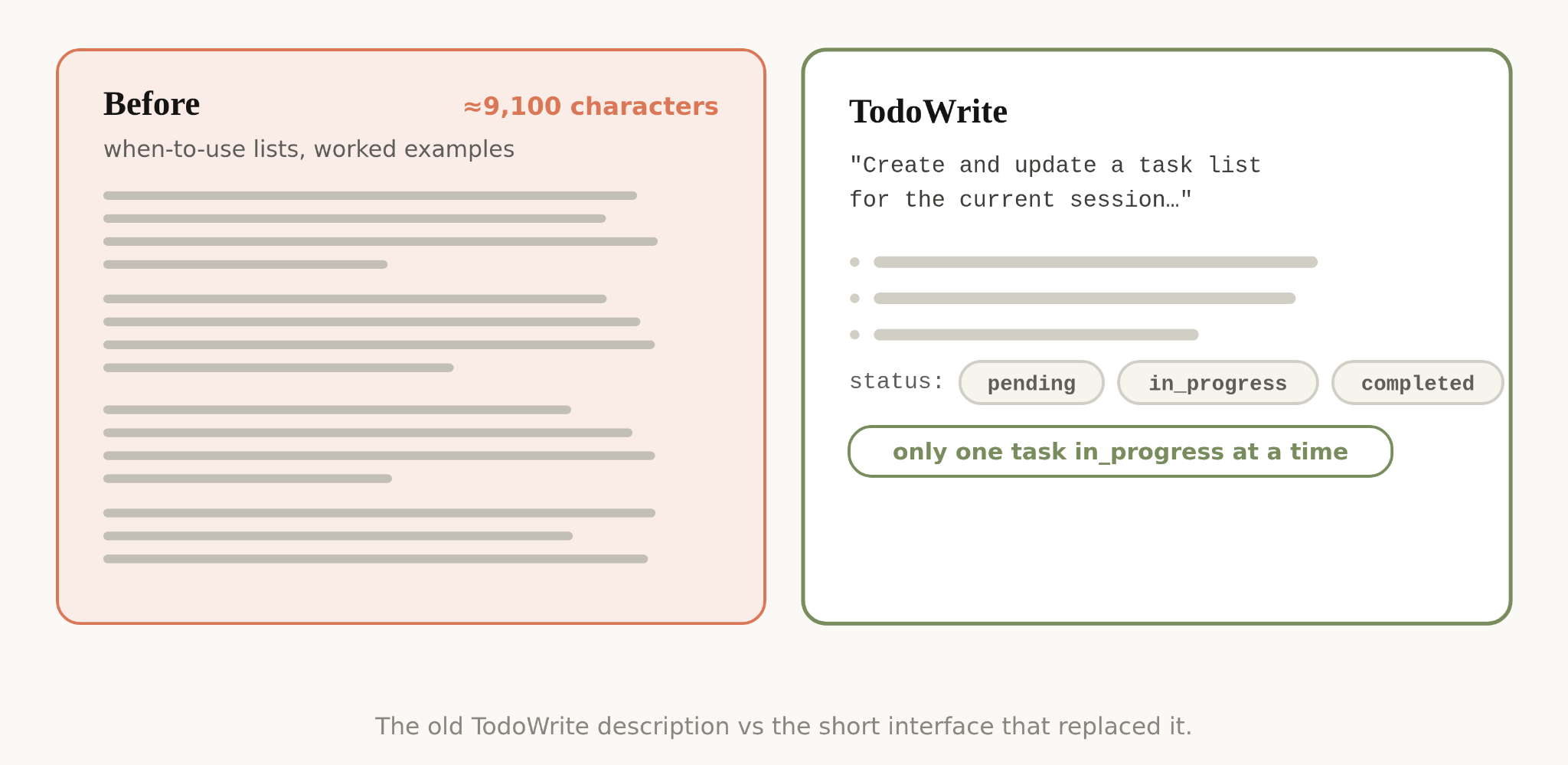
Instead of using examples, think more about the design of your tools, scripts and files- what parameters does Claude have and how can they be more expressive? 

For example, in the Todo tool example, just listing status as an enumeration between pending, in_progress, and completed, hints to Claude about how to use it. The instruction on keeping one item in_progress helps define our requested behavior.

Then: Put it all upfront

Now: Use progressive disclosure

Because Claude Code was focused on coding, our system prompt included detailed information on how to do code review and verification. These were not always needed, but when they were, it was crucial information.

Since then, Claude Code has gotten very competent at using progressive disclosure- loading the right context at the right times. For example, we moved verification and code review into their own skills that Claude Code could selectively call.

But progressive disclosure is not just for skills, we also use it for tools. Some of our tools are ‘deferred loading,’ which means the agent must search for their full definitions using ToolSearch before using them. This allows us to have more tools (such as our Task tools) that don’t take up context until they’re needed.

The same can be applied to your own CLAUDE.md and Skill.md files. A common myth is that you want to make these a central repository for every known practice that you might run into, because Claude would not find it otherwise. Instead, consider having a tree of files that can be loaded at the right time.

Then: Repeat yourself

Now: Simple tool descriptions

Earlier Claude models could sometimes need repeated instructions or be more likely to listen to instructions at the end of their context window than at the start. This meant our system prompt would sometimes have references to tools in the main system prompt as well as instructions in the tool description. 

We found we could delete these repeat examples and put instructions on how to use tools in the tool descriptions rather than the system prompt.

Then: Memory in CLAUDE.md files

Now: Auto-memory

We used to encourage users to save things to Claude’s memory, by using the # hotkey to write to their CLAUDE.md automatically. Instead, Claude now automatically saves memories that are relevant to the work and to you. 

Then: Simple specs

Now: Rich references

In plan mode, Claude Code has heavily relied on markdown files with plans. Storing these files as plans helped Claude refer to them when needed. Another similar best practice was to store specs in the codebase for Claude to refer to while working across longer projects.

But we’ve found that Claude can handle increasingly more complicated references. Instead of simple markdown files, Claude can reference HTML artifacts created by our new artifacts feature. 

You may also give Claude references in the form of code. A spec may also be a detailed test suite, or a function in a different codebase that Claude might port. 

Rubrics are another form of references. Rubrics allow Claude to try and verify your taste in a particular field (e.g. what does a good API design look like) by using dynamic workflows and spinning up verifier agents with those rubrics.

Applying this to your context

Pulling this all together, what does this look like when you assemble your context?

System Prompt

A system prompt is heavily tied to the product context. It tells Claude what product it’s operating in and what it’s doing. For Claude Code, you will likely never modify this, but if you are building your own agent harness, this is where you should spend a lot of time.

CLAUDE.md

Keep your CLAUDE.md lightweight and briefly describe what your repo is for, but spend most of the tokens on gotchas inside of the codebase. For example, you may organize your code to keep types in one monolithic file and nowhere else. Avoid stating ‘the obvious’ things Claude should know by looking at your file system or your repo.

Use progressive disclosure heavily, for example if you have several unique instructions on how to verify your work, create a verification skill and reference it from your CLAUDE.md.

Skills

Think of skills as lightweight guides to let Claude find information when needed. Avoid making them overconstrained, except in highly important areas. 

For long skills, try and use progressive disclosure as much as possible- divide it into many files and split them out.

It’s best when skills encode particular opinions, knowledge, or best practices that are particular to you, your team, or product. 

References

You can @ mention files to include them as references. References allow Claude to refer to in-depth information about the current plan. 

This might be in specs files, mockups, or even entire codebases. Generally you should prefer files that are in code as it provides clear, high-fidelity instructions to Claude in a language it knows very well. For example, a HTML mockup of a design will generally produce better results than a description of the design or a screenshot.

Try simplifying

Across your system prompt, skills, and CLAUDE.md files, you may need to simplify just like we did. We rolled out a new command called claude doctor, which will help you do this automatically as well. For more details on prompting more advanced models specifically, check out our Fable field guide.

The Daily Front Page 6 of 30
Saturday, July 25, 2026 The Daily Front No. #260725 — Cyber Evals
article

UK AISI / Caisi Preliminary Assessment of Kimi K3's Cyber Capabilities

by walrus01·▲ 127 points·45 comments·nist.gov ↗
Kimi K3 performs significantly below the most recent frontier cyber-capable models.

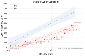
The UK Artificial Intelligence Security Institute (UK AISI) and the U.S. Center for AI Standards and Innovation (CAISI) (UK AISI / CAISI) conducted a joint evaluation of Moonshot AI’s latest model, Kimi K3 (released on July 16, 2026 and slated for open-weight release by July 27, 2026). This evaluation focused on Kimi K3's cyber capabilities and found that:

  • Kimi K3 performs significantly below the most recent frontier cyber-capable models on preliminary cyber evaluations run by UK AISI / CAISI. Specifically:

    • When tasked to develop exploits, Kimi K3 performs significantly below the most recent frontier cyber-capable models (Figure 1).
    • When tasked to attack a simulated corporate network (“The Last Ones”), Kimi K3 performs significantly below the most recent frontier cyber-capable models. Specifically, on average, Kimi K3 reached step 17 of this 32-step attack path, while the most cyber-capable U.S. models reached 28.5 steps on average.
  • Kimi K3 performs above GLM-5.2 on the same preliminary cyber evaluations run by UK AISI / CAISI (Figure 2).

  • Kimi K3’s safeguards allow assistance with agentic cyber exploit development. Kimi K3's safeguards did not prevent it from attempting cyber exploit development or offensive cyber operations during UK AISI / CAISI's evaluations.

Exploit Development Capability

Performance of Kimi K3 and other models on an exploit development benchmark (ExploitBench). Higher success rate indicates greater cyber capability. Error bars represent 95% confidence intervals. ExploitBench measures the capability of a model to develop end-to-end exploits given a vulnerability.

Credit: CAISI/NIST

Figure 1: Performance of Kimi K3 and other models on an exploit development benchmark (ExploitBench). Higher success rate indicates greater cyber capability. Error bars represent 95% confidence intervals. ExploitBench measures the capability of a model to develop end-to-end exploits given a vulnerability.

Detailed Results

These results represent preliminary evaluations on a small set of public and private benchmarks. U.S. closed-weight models were evaluated with system-level safeguards disabled to reduce refusals and enable measurement of maximal capabilities. Publicly available versions of these models have these safeguards enabled. Due to the specifics of Kimi K3’s hosting setup, UK AISI / CAISI ran a selective set of cyber evaluations. Detailed methodologies are provided in individual sections.

Cyber Capability Trends

The cyber capability of models is aggregated across multiple tasks from multiple benchmarks using an approach inspired by Item Response Theory (IRT). For details of the methodology please see prior published reports. Kimi K3’s overall cyber capability has a larger confidence interval than other models because it was estimated from a single benchmark (ExploitBench, which has 41 tasks focused on exploit development). ExploitBench is a leading benchmark to measure a model’s ability to progress along the software exploitation ladder. All other models’ overall cyber capability scores were derived from a larger number of tasks that covered additional domains of cyber capability.

Preliminary comparison of aggregate capabilities over time of the most capable U.S. and PRC models as of Kimi K3’s release. The U.S. trendline is composed of results from frontier U.S. models. A 400-point increase on the y-axis equates to a 10x increase in the odds of solving tasks. Error bars and shaded regions denote 95% CIs.

Credit: CAISI/NIST

Figure 2: Preliminary comparison of aggregate capabilities over time of the most capable U.S. and PRC models as of Kimi K3’s release. The U.S. trendline is composed of results from frontier U.S. models. A 400-point increase on the y-axis equates to a 10x increase in the odds of solving tasks. Error bars and shaded regions denote 95% CIs.

Exploit Development: ExploitBench

ExploitBench is a public benchmark, developed by Carnegie Mellon University, that measures a model’s ability to progress along the software exploitation ladder, including coverage and crash reproduction, arbitrary read/write, control flow hijack, and arbitrary code execution. The benchmark tests models on 41 recent (post-2023) vulnerabilities in the V8 engine (the JavaScript and WebAssembly software that powers Chrome).

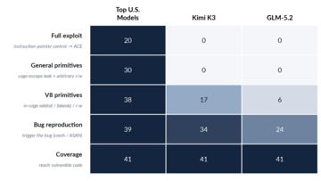
ExploitBench results are presented in Figures 1 and 3.

Detailed ExploitBench performance for Kimi K3 and other models. Darker shading indicates greater cyber capability. Each row represents a key milestone in the exploit development chain, and each cell shows the number of ExploitBench tasks for which the model(s) in question were able to reach that milestone.

Credit: CAISI/NIST

Figure 3: Detailed ExploitBench performance for Kimi K3 and other models. Darker shading indicates greater cyber capability. Each row represents a key milestone in the exploit development chain, and each cell shows the number of ExploitBench tasks for which the model(s) in question were able to reach that milestone.

Kimi K3 outperforms GLM-5.2, the most cyber-capable open-weight model as of June 2026. Kimi K3 achieves a score of 32%, whereas GLM-5.2 achieves a score of 24% (Figure 1).

Unlike the most cyber-capable models, Kimi K3 failed to develop exploits that achieved arbitrary code execution (ACE) for ExploitBench tasks. ACE is the highest-severity outcome in exploit development, granting attackers the ability to hijack a target. Kimi K3 achieved ACE on 0/41 samples, whereas the most cyber-capable models achieved ACE on 20/41 samples on average (Figure 3).

Cyber Range: The Last Ones (TLO)

“The Last Ones” (TLO) cyber range is a 32-step simulated corporate network attack spanning 4 subnets and approximately 20 hosts, which would take a human expert roughly 20 hours to complete. Cyber ranges are expert-built, simulated networks of hosts, services, and vulnerabilities arranged into sequential attack chains that begin at the point of initial network access, and can be used to measure a model's ability to conduct end-to-end cyberattacks autonomously.

On this evaluation, Kimi K3 performs significantly below the leading U.S. cyber capable models. Specifically, Kimi K3 reached step 17 of this 32-step attack path on average, while the most cyber-capable U.S. models reached 28.5 steps on average.

Kimi K3 outperforms GLM-5.2, the most cyber-capable open-weight model as of June 2026. Within the 100M-token limit, Kimi K3 reaches step 17 on average, compared with step 11 for GLM-5.2.

In one of the 10 attempts, Kimi K3 successfully completes “The Last Ones” cyber range within the 100M token limit. This indicates that Kimi K3 is capable of autonomously attacking small, weakly defended and vulnerable enterprise systems, when directed to do so and given initial network access. However, TLO differs from real-world environments in several ways. It lacks active defenders and defensive tooling, imposes no penalty for actions that would trigger security alerts, and contains an intentional attack path.

Solves of TLO are no longer exclusive to a small set of models. In prior testing, four publicly released closed-weight models have solved TLO, with the most capable models solving it more reliably at 6/10 and 7/10 attempts. Kimi K3 solved it in 1/10 attempts within the standard 100M token limit.

The Daily Front Page 7 of 30
Saturday, July 25, 2026 The Daily Front No. #260725 — The Public Mathematician
article

Hannah Fry Wins the Leelavati Prize in 2026 for Mathematics Outreach

by agnishom·▲ 581 points·108 comments·maths.cam.ac.uk ↗
outstanding contributions to increasing the public awareness of mathematics

Congratulations to Professor Hannah Fry, who has been awarded the Leelavati Prize at the International Congress of Mathematicians for outstanding contributions to increasing the public awareness of mathematics.

Hannah Fry is Professor of the Public Understanding of Mathematics in the Department of Applied Mathematics and Theoretical Physics (DAMTP). She joined the University of Cambridge in January 2025, becoming the first person ever to hold the role.

As a broadcaster, author, podcaster and social media star she is one of the UK and world's most recognisable – and favourite – communicators of mathematics and science. The citation for the Leelavati Prize outlines her extraordinary impact: 

"Hannah Fry is one of the foremost global ambassadors for mathematical thinking," the prize citation says. "She has become a voice for mathematics that resonates far beyond the public audience normally interested in science communication.

"Through a wide range of media — including books, videos, and television programs — she has used outstanding creativity and originality to translate mathematics into a language of wonder and relevance for the public without diminishing its scope and importance." 

"When you enjoy [maths] yourself, I think you have first hand experience of just the absolute joy of it," says Hannah Fry about her passion for communicating mathematics. "I feel as though there are these wonderful secrets that are completely invisible to almost everybody in the world who are not mathematicians, and it doesn’t make sense to me we would keep them to ourselves — I feel as though I have this really good bit of gossip that I just want to share."

A language of wonder

The Leelavati Prize, recognising outstanding contributions to increasing the public awareness of mathematics, is awarded every 4 years by the International Mathematical Union (IMU), and is announced at the International Congress of Mathematicians (ICM). Bringing together thousands of mathematicians from around the world, the ICM celebrates the diversity and scope of modern mathematics. It also attracts significant attention as the setting for the announcement of some of the subject's most celebrated awards, including the famous Fields Medals.

The Leelavati Prize is the latest of many honours and awards – across both academia and the mainstream media – recognising Hannah Fry's exceptional work in public communication and engagement. As well as academic recognition including the Christopher Zeeman Medal in 2018 and the Royal Society’s David Attenborough Award in 2024, her major media awards include winning an Emmy in 2025 for an episode exploring quantum computing in the TV series The Future with Hannah Fry, and a Webby Award in 2026 for the podcast The Rest is Science, co-presented with Michael Stevens. With over 2 million followers on Instagram, she has also been named by Time as one of the 100 most influential digital creators of 2026. 

Fry shares the inspiration with the next generation of mathematicians too. In 2019 her televised Ri Christmas Lectures were filmed in front of audiences of hundreds of school children. Even closer to home, earlier this term she gave the annual Rouse Ball lecture to a packed audience of Cambridge students, followed by mathematics communication workshops for current undergraduates.

"Mathematics quietly underpins so many aspects of modern life and the importance of communicating mathematical ideas to the public has never been greater. Few people have contributed more to this goal than Hannah Fry," says Professor Nick Dorey, Head of the Department of Applied Mathematics and Theoretical Physics.

Mathematics is "a completely original way to see the world," says Hannah Fry. "And I think that in the same way as with anything in life where you really enjoy it, I just want to talk to people about it."

As Fry says, the limit to someone's understanding is never their ability to understand. The limit is always in their motivation to care. And she sees her role as being to provide that motivation.

"I think what you need to do," she says about the key to connecting with a wide audience, "is to create a hole in people’s imagination. If I can create just a moment where you want to know the next bit – you know exactly the size and shape it needs to be to fulfil your craving for that exact piece of information – then everybody's in."

Listen to this podcast interview with Hannah Fry about winning the Leelavati Prize, and discover more coverage of the full ICM 2026, on our Plus outreach platform.

Image: Professor Hannah Fry speaking at the Communicating Mathematical and Data Sciences event at the Isaac Newton Institute, Cambridge. Image credit: Grace Merton/INI

The Daily Front Page 8 of 30
Saturday, July 25, 2026 The Daily Front No. #260725 — Small Screen, Big World
article

Building a Tiny 3D Renderer for a Tiny Handheld

by g0xA52A2A·▲ 249 points·20 comments·saffroncr.itch.io ↗
I had no idea how feasible my idea was, so I started with a simple test: a raycaster.

Today I want to talk about my journey writing a 3D software renderer for the Playdate.

At the beginning, I didn't have any performance baseline. I had no idea how feasible my idea was, so I started with a simple test: a raycaster.

I had written one many years ago, based on the code examples from Ken Silverman's webpage, and since then it has basically become what I write whenever I want to test the 3D processing power and screen drawing performance of a low-power device.

You don't need much to write, compile, and run this kind of test, and it gives you a rough idea of the device's processing power. More specifically, it lets you benchmark the areas that matter most for a 3D renderer: how fast it handles floats and vector math, how fast it performs memory operations, how quickly it can draw to the screen, and whether there are any issues with setting up and using a framebuffer.

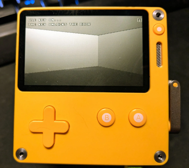
Raycaster running in the simulator

The initial results were worse than I expected. The performance was bad enough that it became clear this was not going to be an easy project.

Raycaster running on the Playdate

To be clear, my raycaster was not written with top performance in mind. This was never about getting a raycasting engine working on Playdate. I'm pretty sure that, with enough optimizations, that can be done. The point was to get a feeling of how much of a powerhouse this device is (or isn't).

This test helped me to get a better understanding of the capabilities of the handheld. It was clear that it didn't have enough power to draw 3D scenes at the level of early 3D accelerators, such as the 3dfx Voodoo, or compete with what you can do on the original PlayStation. But there was hope. The Playdate has a small, low resolution screen, and because it uses a 1-bit display, there are huge memory gains to be had.

From the results I was still confident that I could make something that, from a player's perspective, felt close to the 3DO or Sega Saturn era.

I should clarify what I mean by that. When I talk about something similar to a 3DO or Saturn game, I mean the perceived result on screen. I don't mean it in a technical sense, because the hardware of those consoles is very different from the Playdate.

Both the 3DO and Saturn had custom hardware for drawing polygons (i.e. quads) and modest CPUs. Since the graphics hardware was supposed to do most of the heavy lifting, the manufacturers could get away with a cheaper CPU. The downside was that these machines were not very flexible. They were good at rendering graphics in the specific way their hardware was designed for, but struggled when a game needed a different approach. This is one of the reasons why their Doom ports performed so poorly: Doom's renderer was not a natural fit for the way those consoles wanted to draw 3D.

3DO DOOM

The Playdate, on the other hand, does not have 3D hardware. If we want to render 3D graphics, everything has to be done on the CPU.

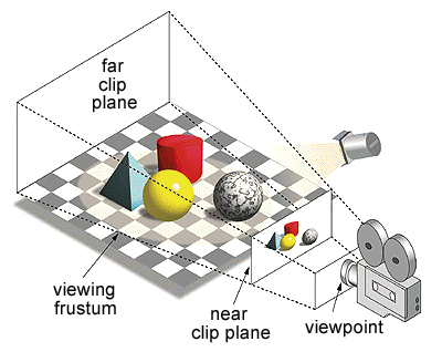
There is no polygon sorting. No rasterization hardware. No depth buffer. No automatic clipping of triangles against the view frustum. No texture mapping, filtering or perspective correction. Nothing.

A quick 101 on 3D graphics

Before going further, it's worth explaining what we actually mean when we talk about 3D graphics.

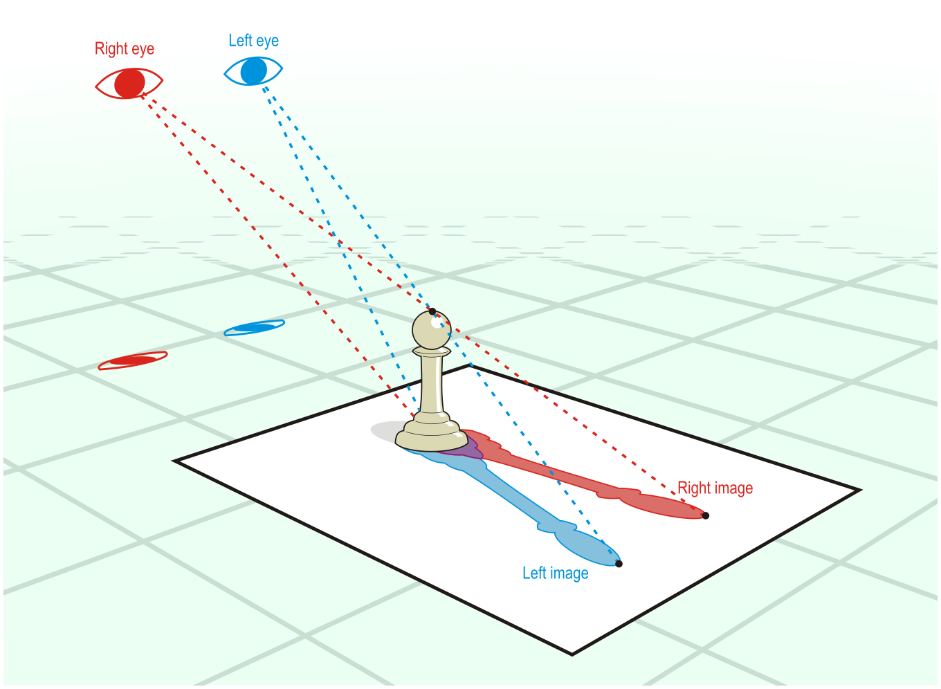
We live in a three dimensional world. Objects have depth, height, and width. They can be far away or close to us, above or below us, to the left or to the right. We are able to perceive these three spatial dimensions and move through them.

But our eyes only receive flat, two dimensional images projected from that world onto the retina. Our brains infer the 3D world through cues such as perspective, motion, scale, shadows, and occlusion.

Eyes looking at a 3d world

Computer graphics use similar tricks.

A 3D game does not draw a world in actual 3D. The screen is flat. Even what we call 3D screens still work by displaying flat, 2D images. What we do is process the information that describes a 3D scene, place a camera inside that space, then project the scene onto a 2D plane, in a similar way to how the real 3D world is projected onto the 2D plane of our eyes.

frustum

The rasterizer is the part of the renderer that takes the projected geometry and turns it into pixels, which is what we use to draw on computer screens. It's the one that figures out how to paint the textures, handles overlapping polygons, clipping, etc. and writes the results in the framebuffer.

That framebuffer contains the 2D image of what we call a frame, and it is what gets displayed on the screen.

On modern hardware, most of this work is done by the GPU. On the Playdate, since there is no GPU, the CPU has to transform the polygon vertices, project them, clip them, sort them, shade/texture them, and write the resulting pixel into the framebuffer. And it needs to do it fast enough to produce a new frame many times per second.

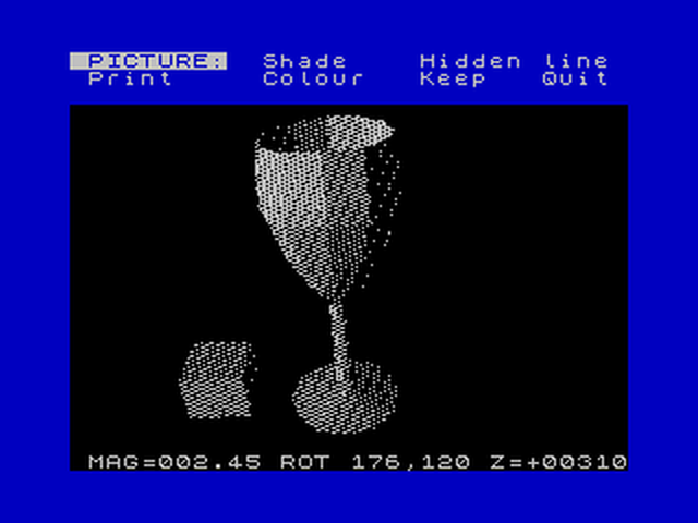
And that's the challenge. The problem is not just "can it draw 3D?". Even a ZX Spectrum can draw 3D, if you give it enough time. The real question is "can it do it fast enough to be playable in real time?".

ZX Spectrum drawing a 3D image

BSPs

My renderer loads Quake BSP map files. I picked this format for two main reasons.

First, it means I did not have to write a level editor and map compiler from scratch. I can use TrenchBroom for level design and ericw-tools to compile the map, visibility data, and lighting. That saves me a huge amount of time.

Second, Quake's BSP format is designed to precompile everything to speed up rendering in slow machines, exactly what I needed.

BSP stands for binary space partitioning. The basic idea is to recursively split space with planes. In 3D, each split divides the world into two half-spaces. Repeating that process creates a tree. Internal nodes contain splitting planes, and the leaves contain regions of space. In a Quake style BSP, those leaves represent convex chunks of the world, and each leaf knows which faces touch it and which other leaves might be visible from it.

BSP

The map compiler does a lot of expensive work ahead of time. It takes the brush geometry, splits it into a BSP tree, computes visibility between leaves, and stores that visibility as the PVS (the potentially visible set). At runtime, the renderer finds the leaf that contains the camera and uses its PVS to reject large parts of the map before rasterization even begins. That's huge time savings.

PVS

The downside is that this approach prefers static worlds. It also requires levels to be designed with visibility in mind. For example, a straight corridor connecting two large rooms may expose too much geometry at once, so an L-shaped corridor is often better because it blocks the line of sight and gives the PVS more opportunities to remove unseen geometry.

Using BSPs made this project much more realistic. Reusing tools saved me time. It's always a good idea to check existing tools and see whether you can reuse and adapt them to your needs instead of reinventing the wheel. Using mature, battle-tested tools for mapping, compilation, visibility, and lighting let me spend my time on the parts of the project that mattered most.

What I made entirely from scratch was the actual 3D software renderer. I didn't want to just port Quake or use someone else's code. I wanted to build it myself so I could be sure I understood it, so I could iterate on it, to test all kinds of ideas, to be able to find the look of the game.

To z-buffer or not

The z-buffer is a depth buffer. A standard depth buffer stores how far away the currently drawn pixel is from the camera. When the renderer wants to draw a new pixel, it compares that pixel's depth against the value already stored in the z-buffer. This is how the renderer prevents distant objects from being drawn over closer ones.

Depth buffer

My first versions didn't use a z-buffer, I tried the classic painter's algorithm approach: drawing from back to front.

But after testing, this version without a z-buffer did not give me meaningful performance gains, it only gave me more headaches.

So I added a z-buffer.

I used a 16-bit reciprocal depth buffer. Instead of storing linear distance directly, it stores a value based on inverse depth. That gives me more precision close to the camera, where small depth errors are easier to notice, and it's large enough to avoid the artifacts I saw when using a smaller 8-bit depth buffer.

The z-buffer also makes dynamic objects and masked textures much easier to deal with. Doors, elevators or pickups can use the same depth test as the level geometry, and cutout textures, such as water, glass, railings or sprites, can simply skip invisible pixels while drawing and depth-testing the visible ones normally.

Water animation

Perspective-correct texture mapping

I experimented with different approaches to see what I could get away with.

The cheapest method is affine texture mapping. With affine mapping, you interpolate texture coordinates directly across the screen. It is fast, but it is only correct for polygons that are parallel to the screen, otherwise, the texture starts to warp. Remember PlayStation textures?

PlayStation texture mapping

In my case the distortion was visible enough. Usually what you do to prevent this is to subdivide your geometry, but I decided against it and benchmark perspective-correct mapping first instead.

My renderer using affine mapping

I went with the classic perspective-correct texture mapping. Instead of directly interpolating the texture coordinates across a polygon (which causes the warping you saw in the PlayStation example), the renderer interpolates values that stay mathematically correct after projection. Specifically, it interpolates 1/z (inverse depth), u/z, and v/z, then reconstructs the actual texture coordinates per pixel by dividing.

This gives accurate looking textures with no warping, but it comes at a cost: every pixel needs a division (reciprocal) to reconstruct the coordinates, which is expensive on the Playdate’s CPU. So I cheat a little: I only calculate the full reciprocal every few pixels, then use a fast approximation for the pixels in between, refining from the previous value. The visual difference is negligible, but the performance win is meaningful, especially since texture mapping is one of the most expensive parts of the renderer.

Perspective-correct texture mapping

Lighting on a 1-bit display

Lighting was one of the strangest parts of the renderer because the Playdate screen cannot show color, not even a grayscale. Each pixel is either black or white.

Quake BSP files include precomputed lightmaps, and ericw-tools can produce improved lighting with features such as bounce lighting and radiosity. My renderer reads that data and converts it into precomputed vertex lighting information that is cheaper to use at runtime.

Still, with a 1-bit display you can only output a black or white pixel. So how do you show brightness on a 1-bit screen?

The answer is dithering.

Dithering is a way of simulating intermediate tones by arranging black and white pixels in patterns. A single pixel is still only black or white, but a group of pixels can look darker or lighter depending on the ratio and placement of those pixels. From a distance, or while the image is moving, the eye blends the pattern into a perceived tone.

Dithering pattern

The renderer uses an 8x8 Bayer matrix. For every pixel, the renderer compares the computed brightness against the threshold value at that pixel's position in the Bayer pattern. If the brightness is above the threshold, the pixel becomes white. If it is below the threshold, the pixel becomes black.

Across an area, this creates the impression of grayscale, even though the final image uses only black and white.

The hard part is that dithering can easily become noise. A fully textured, fully lit scene may be technically impressive but visually hard to read on a 1-bit display. And that was my next fight.

Doom 1-bit noise

Finding the right look

One of my main visual references was Return of the Obra Dinn. I also love the look of Jet Set Radio. So from the start I knew I wanted strong outlines and simple textures. Kind of a 1-bit cel-shading look.

Return of the Obra Dinn

Jet Set Radio

I still tested the default approach: standard textures, applying lighting and then 1-bit dithering.

Test map in the editor

Renderer with too much noise

As I suspected, it was too noisy. The geometry and textures were hard to read. With more iterations, it could have been improved, but that test proved to me that the minimalist, cel-shaded approach made more sense.

Then I tested the map using simple textures and strong outlines, the 1-bit cel-shading look.

1-bit cel-shading look

1-bit cel-shading look

1-bit cel-shading look

That immediately improved readability. And most importantly, it gave the game a stronger identity. I loved the look. I knew this was the way.

The textures look a bit silly in the map editor, but they work in-game, which is what matters.

Silly textures in the editor

Silly textures in-game

Optimization time

I tried all kinds of tricks and ran benchmarks for every change, trying to find the best approach for the Playdate. These are my findings:

  • Using these compiler flags improved performance in a noticeable way:

    • -mcpu=cortex-m7 -mthumb Tells the compiler to generate and tune code specifically for the ARM Cortex-M7 CPU used by the Playdate.

    • -mfpu=fpv5-sp-d16 Tells the compiler the exact FPU the Playdate has, to generate the appropriate float instructions.

    • -mfloat-abi=hard Enables the hard-float ABI, this allows float values to be passed through FPU registers, reducing overhead.

    • -Ofast Enables very aggressive optimization. On Playdate, smaller code can sometimes run faster than more aggressively optimized code, so I benchmarked this against -O2, -O3, and -Os before choosing it.

    • -Wl,--gc-sections -flto -fdata-sections -ffunction-sections This helps strip unused code from the device build, reducing binary size, optimizing cache use.

    • -fno-unwind-tables Reduces binary size by removing stack-unwinding metadata that the game does not need at runtime.

    • -fno-asynchronous-unwind-tables Removes more metadata from the binary, keeping the device build smaller.

    • Playdate's recommendations:

      • -Wdouble-promotion It warns when a float is implicitly promoted to double, IMO this is always useful but in this case we really want to avoid using doubles by mistake.
      • -fsingle-precision-constant This makes any floating point constant value single value by default. I always use x = 0.1f instead of x = 0.1 but again, it's a good idea to make sure we don't use doubles.
  • Using ARM Cortex-M7 assembler for floating-point instructions. I created my own custom floor, ceil, sqrtf, and fabsf functions.

  • Half resolution rendering: I render internally at 200x120, then scale to the Playdate's 400x240 screen. This is one of the biggest performance gains.

  • I use precomputed values and caches for anything that can be calculated outside of the game loop. Don't spend time every frame on calculations that can be done once. Seriously.

  • For the most critical functions I use these two macros:

#if TARGET_PLAYDATE 
#define PD_HOT __attribute__((section(".text.hot"))) __attribute__((aligned(32)))
#define PD_FORCEINLINE inline __attribute__((always_inline)) 
#else #define PD_HOT 
#define PD_FORCEINLINE inline 
#endif
  • PD_HOT places performance critical code in a dedicated section and aligns it during linking, which helps to improve instruction cache.
  • PD_FORCEINLINE is used for small, frequently called functions. The compiler replaces the function call with the function body, avoiding call overhead.
  • Both should be used only when needed. Overuse may increase code size and hurt the cache making the code run slower. Again, benchmarks were essential to decide when they were actually useful.
  • And last but not least, my favorite piece of optimization advice, from Michael Abrash's Graphics Programming Black Book:

The best optimizer is between your ears

If you want to optimize your Playdate game, treat everything I wrote here as an idea, not as objective truth. The things that worked for me may not work for you, and you may need to make different changes. Run your own benchmarks, and make sure every optimization you keep is actually doing something.

Remember: the best optimizer is you.

Perfect is the enemy of good

Writing a 3D renderer for the Playdate has been a long and fun journey. I wasn't sure if it was even possible at the start. And each time I tried something, it ran so slowly that it was hard not to feel a bit demotivated. But I pushed on.

My current renderer is far from perfect, but it's good enough. If you want to make actual progress, try to aim for "good enough".

Getting the renderer to a playable state has allowed me to start prototyping gameplay ideas. It has allowed me to get a playable prototype that is starting to feel like an actual game. And as a game developer, that's what matters.

Thanks for reading, and have an excellent day!

The Daily Front Page 9 of 30
Saturday, July 25, 2026 The Daily Front No. #260725 — The Halftone Habit
article

How My Images Are Dithered

by surprisetalk·▲ 236 points·76 comments·dead.garden ↗
I don't know much about dithering.

How my images are dithered

I don't know much about dithering. But when I visit other people's sites and they dither their images in cool ways I always wonder how they do it. So in case anyone is wondering, here's my current method for dithering these pink images.

Edit: Almost like I know myself too well — the pictures now look like this instead: my friends at a restaurant, the colors are normal-ish (not pink), except it's a bunch of dots

Which is covered in the post.


Welcome to all the hacker news readers who clicked on this post. I am thankful and glad that this post has come to entertain some of you. Here are some things I feel the need to add to the post since it has left my regular audience:

  • There seems to be discussion about whether this counts as dithering. As evidenced by the very first sentence of the post, I am not an authority on the subject. But here is what Wikipedia seems to think:

    Dithering is analogous to the halftone technique used in printing. For this reason, the term dithering is sometimes used interchangeably with the term halftoning particularly in association with digital printing. (link)

    In any case — I am/was only aware of this technique being used for AM grid printing, as briefly layed out in the post. So I thought it might be fun to play pretend a little.

  • this is a very inefficient method of reducing the size of an image file — I'd even say this little experiment has nothing at all to do with decreasing file size (in some unlucky cases it will even increase the size of your image). I mention this a few times in the post. It's just a bit of playing around with a certain aesthetic

  • please don't feed images of me and my friends to an LLM?? The code for achieving each effect is all over this page. Just make your own image and feed that to an LLM.

Dithering, beside making a picture look (to put it professionally) cool as fuck, can also reduce file size (by using less colors while maintaining details) and thus needed storage (if using only the reduced images) and the weight of your website for the client. That's why sites like Low Tech Magazine use it, for example.

The idea of pink images came from a post a while back, when I tried this before. The post Designing without color introduces the idea of the current design, where I try to get a sort of black and white "printed" vibe, using color only for emphasis. (This makes sense only when you are a light mode user like me).

The image back then, with the old method, looked like this: The brightest color here is now a mid-range pink, the one I use for marking text on the site

The key difference here being that I limited the picture's palette to true monochrome: black and this pink. Also, the weird "dithered" dots are much bigger.

So what's this

Zoom in on the Chrome logo being displayed on an LCD screen My goal was to immitate a printed image. While individual pixels on a screen may have the luxury of setting variable values of red, green and blue — making the grid of repeating RGB lights on your screen light up with different intensity — things work a little differently on paper (and other print substrates).

Getting the limited palette of colors your printer is working with to give the illusion of more colors requires using a grid/matrix of dots. You can go about this in three different ways: AM, FM and hybrid grids. The amplitude here being the size of the dot and the frequency, well … the frequency. Making a dark spot with AM grids means big dots, in FM grids it's lotsa dots.

The top shows an FM print: the dots look chaotic.

The bottom shows AM: all dots show up in a predictable pattern and light spots have smaller dots

The problem with amplitude modulated dots is that if you approach this naively you will end up getting unwanted patterns in your images: a so-called Moiré.

Example of unwanted pattern resulting from stacking two grids on top of eachother

For this reason, there is a rule (DIN 16547) about how exactly the colors are to be offset in an AM print to try and avoid them getting in each others way. Since FM grids are random they do not suffer from this problem.

Yellow at 0°. Cyan at 15°. Key (Black) at 45°. Magenta at 75°

Simulating AM pattern on your digital image

I access my server via the command line — so I use a command line tool to quickly edit images. The tool is called imagemagick and is called using the "convert" command.

I found the method to create this illusion online (can't find the link) and adapted it a little. So I can't claim to be the expert on what each individual argument does, but I will try to explain it.


convert "oldfile" -resize 800 -set option:distort:viewport '%wx%h+0+0' \
                 -colorspace CMYK -separate null: \
                 \( -size 2x2 xc: \( +clone -negate \) \
                +append \( +clone -negate \) -append \)  \
                -virtual-pixel tile -filter gaussian  \
                \( +clone -distort SRT 2,0 \) +swap  \
                \( +clone -distort SRT 2,15 \) +swap   \
                 \( +clone -distort SRT 2,45 \) +swap  \
                \( +clone -distort SRT 2,75  \) +swap +delete \
                -compose Overlay -layers composite -set colorspace CMYK -combine \
                "newfile"

Here's what it does generally: resizes the image to 800px in width (who needs more?), sets the color to CMYK, applies a background to fill the empty space left by rotating (and sets a gaussian blur to filter noise), splits up into the colors, scales them up a bit (for bigger dots) and distorts them (in this case: rotates them) and at the end it combines the 4 images into one again.

The image we generate by running this on the original file looks like this:

there is a resemblance to the targeted goal

Before combining them, these are the individual colors dot grids:

This sets C at 0°, M at 15° etc. But whatever. Zooming in and out doesn't make any weird artifacts apparent so it's good enough.

If we increase the size of the dots to a ridiculous degree (8x8), you can get a better look at what is happening.

square soup

Edit: The perfect route to CMYK

After sleeping on it and reading the post back, the solution for a pic limited to truly CMYK colors in an AM grid is apparent. For reasons I get into later this is NOT a good way of reducing file size (apart from the fact that limiting colors and resizing the image to 800 in width always reduces the size, everything else is pretty much stacked against that goal). It does, however, look cool.

With the above method, the dots do not vary in size. Why should they? As we already discussed, a digital image (unless I have a GIF or PNG-8 situation somewhere) can give varying intensity of light for R, G and B per pixel. So when we look at the big image above we can cleary see some of the squares are just darker than others. For a true immitation this will not do!

All we need to do is to limit each channel's colors to 2 before combining them again. This is very obvious in hindsight. Idk why the person I got the original command from didn't do this.

convert "oldfile" -resize 800 -set option:distort:viewport '%wx%h+0+0' \
                 -colorspace CMYK -separate null: \
                 \( -size 2x2 xc: \( +clone -negate \) \
                +append \( +clone -negate \) -append \)  \
                -virtual-pixel tile -filter gaussian  \
                \( +clone -distort SRT 2,0 \) +swap  \
                \( +clone -distort SRT 2,15 \) +swap   \
                 \( +clone -distort SRT 2,45 \) +swap  \
                \( +clone -distort SRT 2,75  \) +swap +delete \
                -compose Overlay -layers composite -colors 2 -set colorspace CMYK -combine \
                "newfile"

This will produce an image that looks like this:

now that's what I'm talking about

In retrospect I wonder if I might try out images like this instead of pink. If all I want is the general vibe of the grid then pink is fine. Though it does have more colors (shades of pink) for less colors (actually useful distinct ones). Who said blogging about your stupid idea isn't useful?

Pink — old method

The script for the old way of doing it had the values of -distort SRT set to "2 (rotation)", meaning it scaled the colors up to 2, making bigger dots.

After running the script above, the colorspace was once again converted, to Gray this time, after which the colors were leveled to monochrome: black and this pink. The whole command for those who want to try:


convert "oldfile" -resize 800 -set option:distort:viewport '%wx%h+0+0' \
                 -colorspace CMYK -separate null: \
                 \( -size 2x2 xc: \( +clone -negate \) \
                +append \( +clone -negate \) -append \)  \
                -virtual-pixel tile -filter gaussian  \
                \( +clone -distort SRT 2,0 \) +swap  \
                \( +clone -distort SRT 2,15 \) +swap   \
                 \( +clone -distort SRT 2,45 \) +swap  \
                \( +clone -distort SRT 2,75  \) +swap +delete \
                -compose Overlay -layers composite -set colorspace CMYK -combine \
                -colorspace Gray -colors 2   +level-colors  black,#A2719B \ 
        "newfile"

If we zoom in on the image before and after leveling the colors, we can see the dots do seem more like they vary in size. I omitted the -resize flag to give you a better view of the details.

CMYK detail Pink detail

While not entirely accurate, I think this method gets the most printy feel out of an image. Sadly it can swallow a lot of detail, even if the dots aren't scaled up. So I abandoned this after a while (also I got sick of looking at it).

Edit: now compare to the real deal:

the new method limits the colors to CMYK for real, making the dots vary in size across four channels

Pink – new method

it is made up only of shades of pink, as well as black and white. the vague pattern from the method I got online can be seen but the dots do not look like they vary in size

Monochrome is a cool idea but just has limited use for the blog (and other pics on the website). I need some more depth. What I need is more values of pink. I get these by utilizing the -remap flag.

A linear gradient going through this site's whole color palette: white, black, pink and darker pink


convert "oldfile" -resize 800 -set option:distort:viewport '%wx%h+0+0' \
                 -colorspace CMYK -separate null: \
                 \( -size 2x2 xc: \( +clone -negate \) \
                +append \( +clone -negate \) -append \)  \
                -virtual-pixel tile -filter gaussian  \
                \( +clone -distort SRT 1,0 \) +swap  \
                \( +clone -distort SRT 1,15 \) +swap   \
                 \( +clone -distort SRT 1,45 \) +swap  \
                \( +clone -distort SRT 1,75 \) +swap +delete \
                -compose Overlay -layers composite -set colorspace CMYK -combine \
                -remap "$palette" -colors 32 "newfile"

Problematic images

For images like the one I've been using everything works beautifully. But with images that are very overwhelmingly light, there can be issues.

Here's an example:

Original image

After running script

After manual edit

The edit in question: increasing brightness to 300%, Saturation to 200%, inverting colors and remaping them to pink

convert "oldfile" -modulate 300,200,100 -negate -remap $palette "newfile" 

This is possibly because my color palette is kinda bad.

Is this even dithering?

If all you care about is the result then you could say the image has been dithered, especially in the old method. Using only two colors we created the illusion of semitones (is this appropriate usage in English?)*. The same is basically true for the new method as well.

* I looked it up, the translation in this case is, in fact, simply "half tones" :^)

But if you care about the method this is not dithering. Or at least it's the most unnecessarily computationally expensive form of dithering I've come across. Let's walk through the steps one more time:

  1. Convert RBG to CYMK, adding one channel
  2. Split the image into four images and transform each one (starting with scaling them up and inverting them)
  3. limit colors to 2 on each and then overlay four images on top of eachother
  4. set colorspace to CMYK again
  5. limit the colors to 32/64/not sure yet where I want this (overlaying the 4 grids will create new colors)

This whole thing, on my laptop with an 11 year old CPU, can take 10 seconds if the image is big. The file size is not exactly "small" (though still smaller than unscaled pics with more than 32 colors). I can imagine the pattern isn't doing compression algorithms a huge favour. If you value your time or care about actually reducing an image's size do not do this.

Script

#!/bin/bash
temp="/tmp/images"
palette="/path/to/palette.png"
rm $temp
if [[ $1 = "" ]]; then
if [ -d smol ]; then 
echo must run with argument
else 
mkdir smol big
ls -r *.webp > $temp
ls -r *.png >> $temp
ls -r *.jpg >> $temp
ls -r *.jpeg >> $temp
ls -r *.gif >> $temp
fi
else 
ls -r *$1 > $temp
cp *$1 big
cat $temp
cp $(cat $temp) big/.
fi
i=$(cat "$temp" | wc -l)
echo $i
    while [[ $i -gt 0 ]]
    do
name="$(head -n $i $temp | tail -n +$i)"
echo "doing $name"
convert "$name" -set option:distort:viewport '%wx%h+0+0' \
         -colorspace CMYK -separate null: \
         \( -size 2x2 xc: \( +clone -negate \) \
        +append \( +clone -negate \) -append \)  \
        -virtual-pixel tile -filter gaussian  \
        \( +clone -distort SRT 2,0 \) +swap  \
        \( +clone -distort SRT 2,15 \) +swap   \
         \( +clone -distort SRT 2,45 \) +swap  \
        \( +clone -distort SRT 2,75 \) +swap +delete \
        -compose Overlay -layers composite -colors 2 \
        -set colorspace CMYK -combine \
        -colors 64 "smol/$name"
(( i-- ))

echo $i
done

To end with, here is the original image with actual dithering (FloydSteinberg)

This file is smaller than the new (pink) method (but bigger than the old one).

Edit: the true method will produce a smaller file for this image :^} (though this is not a rule!)

(Edit:) RGB

You can ofc do the same thing with RGB instead of CMYK. That wouldn't really be as accurate for a "print vibe"!! but here's the RGB AM grid version:

the image has darker, more intense colors and more details at some places

The Daily Front Page 10 of 30
Saturday, July 25, 2026 The Daily Front No. #260725 — Collision Course
article

SIMD for Collision

by birdculture·▲ 108 points·29 comments·box2d.org ↗
I like to call this approach “wide SIMD”.

In a previous post SIMD Matters I discussed the big wins I got from graph coloring to make the contact solver faster. That same approach exists in Box3D. I like to call this approach “wide SIMD”. The idea is to process multiple work units at the same time. In the contact solver this means solving four contact points at the same time.

This is different from “narrow SIMD” where a 3-vector (xyz) is put into a SIMD register and then standard vector math is expressed as SIMD intrinsics. Narrow SIMD can be useful, but the gains are not as obvious.

In 3D there is an opportunity for using wide SIMD that doesn’t exist in 2D. Consider the convex pile benchmark ported from PEEL. This benchmark drops 5120 convex hulls, each with 32 points.

Convex Pile

Box3D treats boxes as hulls and many of the benchmarks use boxes. The performance with boxes has been good and typically most of the cost is not in the narrow phase. But the 32 point hull is a different beast. Let’s call it “boulder”. The table below shows the hull details for a box compared to the boulder.

Hull Vertices Faces Edges Box 8 6 12 Boulder 32 59 89

Box3D uses the Separating Axis Test for collision detection. This is abbreviated as SAT. Using SAT I can find the best features to use for pushing the shapes apart and precisely how far apart they need to be pushed to remove overlap. Furthermore, I use these results to compute the contact normal and the contact points.

Other physics engines may use the distance algorithm GJK instead with an overlap fallback such as the Expanding Polytope Algorithm, also known as EPA.

I’m a big fan of SAT for convex hull collision because it doesn’t require a collision margin. Shapes can rest directly on each other. The GJK and EPA combo usually tries to keep shapes slightly separated to stay in the GJK region, which is faster. This can lead to visual gaps. Also, EPA can be numerically brittle and often physics engines will need a fallback if EPA fails: a fallback for the fallback. EPA is essentially an algorithm for computing a convex hull, and the input data can be flat slivers. That is a challenging scenario for convex hull computation. Hence the need for a second fallback.

Unfortunately, SAT in 3D has quadratic complexity. With two hulls A and B, the collision algorithm must test the faces of hull A against the vertices of hull B, the faces of hull B against the vertices of hull A, and the edges of hull A against the edges of hull B. In the worst case, every combination must be evaluated.

Combination Face-Vertex Vertex-Face Edge-Edge Box-Box 6 6 144 Boulder-Boulder 59 59 7921

The number of edge-edge combinations grows quadratically. There are some tricks to speed up the edge tests using the Gauss Map. See Improvements to the Separating Axis Test for more details. Regardless, the edge-edge test can easily dominate the entire simulation.

So what does this edge-edge code look like? At a basic level it looks like this:

for (Edge edgeA : hullA.edges)
{
    for (Edge edgeB : hullB.edges)
    {
        TestCrossProduct(edgeA, edgeB);
    }
}

If there are just 12 edges in each hull, doing SIMD on this is not a big win because SIMD requires some setup work. For SIMD to work well the data needs to be in structure of arrays format (SoA).

With 89 edges in each hull the story changes drastically. There are 7921 calls to TestCrossProduct. With wide SIMD I can test one edge of hullA against four edges of hullB simultaneously. It looks sort of like this:

for (Edge edgeA : hullA.edges)
{
    for (EdgeWide edgeWideB : hullB.edgesWide)
    {
        TestCrossProductWide(edgeA, edgeWideB);
    }
}

There are a lot of hidden details in the snippet and you can look at the Box3D code if you are curious. But I’m here to answer the question: should we care about SIMD for collision detection? Well, I have results! These are the results for the convex pile benchmark with the total milliseconds for a 500 step run. I tested 1 to 8 threads on an AMD 7950x with the CPU pegged at 4.42GHz. The results are the best of 4 runs.

Threads Scalar SSE2 AVX2-Lite 1 40706 17337 15762 2 20799 8857 8131 3 13789 5946 5471 4 10324 4509 4084 5 8359 3675 3361 6 6958 3106 2843 7 6006 2697 2477 8 5292 2410 2277

SSE2 is over twice as fast as scalar! Keep in mind these timings are for the entire simulation, not just the edge-edge test. The scalar column also indicates that the contact solver runs in scalar mode. So this is the full picture of the simulation.

Box3D only implements SSE2 intrinsics. In Box2D I have AVX2 intrinsics as well, but there were a surprising number of users without AVX2 capable CPUs. Nevertheless, just enabling the AVX2 architecture in Box3D gives a nice gain, as indicated in the AVX2-Lite column. Free performance gains are great to see. In the future I may try a real AVX2 implementation testing 8 edges at a time.

This benchmark represents a 32-point hull with 89 edges. Surely SAT will be overrun as the point count grows further. Well, fortunately Box3D has a hard 128 edge limit. This limit already existed and has to do with keeping the hull storage compact (8-bit indices and two half-edges per edge). Somewhat surprisingly, converting complex hulls to meshes can solve the quadratic growth problem, but it makes the shape less suitable for a dynamic body.

You may wonder if the SIMD edge tests moved the needle on box-box. Sadly it has almost no effect. This optimization seems to only benefit complex hulls. Such hulls can come up in several scenarios, such as destruction. So it is a worthy addition to Box3D.

Finally, here is a video comparison and a side-by-side of the frame timings.

Frame Timings

The Daily Front Page 11 of 30
Saturday, July 25, 2026 The Daily Front No. #260725 — Code in Two Dimensions
article

Spatial languages: Writing code in 2D

by BinRoo·▲ 110 points·40 comments·shukla.io ↗
what happens when we unlock an extra dimension?

I guess expressions don’t really need to read left-to-right on a line.

Why can’t a < b be written vertically too?

a
<
b

All this time we’ve been writing expressions in 1D space, but what happens when we unlock an extra dimension?

Of course the IDE and parser need to play nicely for all this to work. Even then, what’s the point? Well, let’s take a look at these examples below.

3-arity functions

We don’t really see 3-arity functions written in infix notation much.

For example, in Python (and most other languages), you can and 3+ things at once:

x and y and z

Technically, that’s just composing multiple binary functions together.

Even this shortcut in Python to simplify (a < b) and (b < c) is more of the same thing:

a < b < c

Now, let me introduce you to a funny little operator I’ve been playing with called andFlip, which motivates the need for a true 3-arity infix notation. First, here’s the definition of the function:

def andFlip(args):
    if args[0] and args[1]:
        args[2] = not args[2]
    return args[2]

It takes 2 inputs and flips the target if both inputs are true.

There’s just no good way to write this with infix notation. But let’s try anyways!

Define @@ to be the infix symbol for the andFlip operator. What does it look like in practice?

Method 1: the standard way

One option is to curry andFlip: the infix @@ takes 2 args and returns a function awaiting the 3rd, like so:

(a1 @@ a2) a3

Yeah, that’s alright. It works. But…

Method 2: the goofy way

Forget what you know about code for a second. If I could flick a magic wand, I’d wish for the 3-arity notation to look like this:

   a3
a1 @@ a2

Might as well make use of the y-axis, right?

It makes chaining so much easier:

t1 = 0
t2 = 0

   t1    t2
(x @@ y) @@ z

In the chain, x @@ y toggles t1, and t1 continues the chain t1 @@ z, which toggles t2.

That’s a successful three-way toggle, where all x, y, and z must be true for the target to toggle.

Btw, since we’re working in 2D space now, the following expression,

  t1
x @@ y

is equivalent to:

x @@ y
  t1

Example: my chicken coop door

Consider the automatic door I’ve installed on my chicken coop.

The coop’s automatic door (right) and its controller box

The coop’s automatic door (right) and its controller box

With just a photometer and its internal clock, the microcontroller tracks:

  • x – the photometer crossed its dusk/dawn threshold
  • y – the reading has held steady for five minutes
  • z – the gate has not recently toggled

The door toggles only when all three line up. A passing cloud trips x but never outlasts y, so the door stays put.

The coop’s controller is the same chained expression from above:

t1 = 0
t2 = 0

   t1    t2
(x @@ y) @@ z

You might be wondering, why not just write x and y and z? Because then the door would mirror the sensors, swinging right back the moment a condition fades. @@ toggles in place: the door moves once and stays, and the partial answer lands in t1, a scratch bit.

Spatial languages get even more fascinating when we introduce vertical chaining!

Vertical chaining

That mutable variable t1 disqualifies the expression from being called a “pure function”. But can we fake it? Can we reset t1 back, all within the same expression?

I’d like to introduce vertical chaining through two puzzles.

Puzzle 1: reset t1 back to 0

As mentioned, in the chaining examples above, the variable t1 is mutable.

Here’s a puzzle: how can we reset it back to 0, so the expression “appears” immutable?

You may be tempted to just append the statement t1 = 0 and call it a day, but the goal of the puzzle is to do it all within the same expression.

Give it a shot before you scroll down!

Here’s the answer. Since t1 can be reset by repeating the same thing that was used to toggle it, we can combine expressions into a larger 2D one, like so:

t1 = 0
t2 = 0

(x @@ y) @@ z
   t1    t2
(x @@ y)

Ok, I’m probably blowing your mind right now.

The data flow is still as you’d expect in a programming language, left-to-right and top-to-bottom. If x and y are true, the first x @@ y flips t1 and then the second x @@ y resets it. Otherwise, both leave t1 untouched.

This puzzle actually models the CCCX gate in quantum computing, where uncomputing the intermediate t1 value within the same circuit is an important requirement.

Puzzle 2: reset the temporary variable back to the original value

If t1 starts off with an unknown boolean value n, then it gets more complicated.

t1 = n
t2 = 0

   t1    t2
(x @@ y) @@ z

The same trick above to reset t1 back to its original value won’t work.

See for yourself: when t1 = 1 and x, y, and z are all true, then t2 remains 0, which is incorrect.

t1 = 1
t2 = 0

(1 @@ 1) @@ 1
   t1    t2
(1 @@ 1)

So, what’s the answer?

Tada!

t1 = n
t2 = 0

   t1    t2
(x @@ y) @@ z
   t1    t2
(x @@ y) @@ z

Absolutely legendary. This single 2D expression resets t1 back to n while producing the correct result for t2.

This puzzle is inspired by the concept of resetting a borrowed ancilla in quantum computing. t1 is the “borrowed” or “dirty” value that remains unchanged.

Here’s the same circuit in Qiskit:

from qiskit import QuantumCircuit, QuantumRegister

x = QuantumRegister(1, "x")
y = QuantumRegister(1, "y")
z = QuantumRegister(1, "z")
t1 = QuantumRegister(1, "t1")  # starts in unknown state n
t2 = QuantumRegister(1, "t2")  # target, starts at 0

qc = QuantumCircuit(x, y, z, t1, t2)

qc.ccx(x, y, t1)
qc.ccx(t1, z, t2)
qc.ccx(x, y, t1)
qc.ccx(t1, z, t2)

I’d argue that the Qiskit implementation is harder to follow, because of the back-and-forth variable tracking.

By the way, here’s the corresponding quantum circuit diagram:

wires: x, y, z, t1 = n, t2 = 0
outputs: x, y, z, n, x·y·z
ccx x y t1
ccx t1 z t2
ccx x y t1
ccx t1 z t2

In some ways, this circuit diagram is easier to follow, but probably not scalable.

The spatial language syntax is the best of both worlds.

Defining new operators

First, meet @@’s little sibling. A single @ takes one condition instead of two: x @ y flips y whenever x is true.

With @ and @@ in hand, we can define new operators, spatially. The left side of := is a shape, and the right side is what that shape rewrites to:

b maj c        (a @ b) @@ (a @ c)
  a       :=            a

This strange operator flips both b and c when a is true, and then flips a if both sides came out true. That computes a ^ ((a^b) & (a^c)) into a, which happens to equal the majority of the three inputs, which is why this operator is called maj.

And maj is no arbitrary choice. It’s the MAJ gate from the classic quantum ripple-carry adder, where the majority of (carry, bit, bit) is the next carry.

You may have noticed that maj leaves b and c dirty, holding a^b and a^c, the same kind of mess as our borrowed t1. To clean up, we’ll also introduce uma, the partner operator. The name comes from the same adder paper, “UnMajority and Add”: it un-majorities c, restores a, and adds the sum onto b:

c uma b        ((b @@ a) @ a) @ b
  a       :=        c

Let’s see what happens when we wire them up.

3-bit adder

We can build a 3-bit adder out of three majs that ripple the carry up through the a wires, with the final @ dropping the carry-out on c3, and finally one line of umas resetting all the scratch wires:

c0 = 0
c3 = 0

(b2 maj (b1 maj (b0 maj c0))) @ c3
    a2      a1      a0
((  .       uma b2) uma b1) uma b0
                            c0

That’s a full 3-bit adder in a single 2D expression that also cleans up after itself. The b wires now hold a + b, c3 holds the carry-out, and c0 and the a wires come back exactly as we found them. (Set c0 = 1 and you get a + b + 1 for free.)

Notice the two lines mirror each other. The top nests rightward down to b0 and ripples the carry back up; the bottom nests leftward down to b2 and unwinds back out. The shared a1 and a0 labels are the pivots, each serving the maj above it and the uma below it, and the . is a vertical pipe, standing for whatever wire sits directly above it, here a2. The carry chain is stitched together vertically: the uncompute touches the compute, just like in the puzzles.

Speedrunning other spatial languages

Here’s a quick tour of a few more spatial languages.

Befunge

The grandparent of 2D languages (Befunge, 1993): the instruction pointer physically travels the grid, and >v<^ steer it. Hello world bounces off the walls:

>              v
v"Hello World!"<
>:v
^,_@

Orca

Orca is a livecoding sequencer where every letter is an operator that reads its neighbors: A adds the value to its left and the value to its right, and writes the sum directly below itself. Sound familiar?

1A2
.3.

Racket #2d

A real, shipping language extension: Racket’s #2dcond is a cond evaluated in two dimensions. The left column tests b, the top row tests a, and the cell where both are true runs.

#lang 2d racket

(require 2d/cond)

(define (same? a b)
  #2dcond
  ╔═════════════╦═══════════════════════╦═════════════╗
  ║             ║       (pair? a)       ║ (number? a) ║
  ╠═════════════╬═══════════════════════╬═════════════╣
  ║ (pair? b)   ║ (and (same? (car a)   ║     #f      ║
  ║             ║             (car b))  ║             ║
  ║             ║      (same? (cdr a)   ║             ║
  ║             ║             (cdr b))) ║             ║
  ╠═════════════╬═══════════════════════╬═════════════╣
  ║ (number? b) ║          #f           ║   (= a b)   ║
  ╚═════════════╩═══════════════════════╩═════════════╝)

Hexagony

Hexagony runs on a pointy-topped hexagonal grid, like a certain background you may have noticed. Six instruction pointers start at the six corners. Hello world:

   H ; e ;
  l ; d ; *
 ; r ; o ; W
l ; ; o ; * 4
 3 3 ; @ . >
  ; 2 3 < \
   4 ; * /

Ladder logic

Ladder logic is how PLCs run factories (and, done properly, chicken coop doors): each rung is a relay circuit read rail-to-rail, and parallel branches are OR. This classic seal-in rung computes Run = (Start OR Run) AND (NOT Stop):

--+----[ ]--+----[\]----( )
  |   Start |   Stop    Run
  |         |
  +----[ ]--+
       Run

And an honorable mention for the most successful spatial language of all time: the spreadsheet, where every formula lives at a 2D coordinate and reads its neighbors.

“This Is Water”

If you know me, you know I love bringing up the Sapir-Whorf hypothesis, which proposes that language shapes the way you think:

  • Some Australian Aboriginal languages have no words for left and right, only compass directions, so their speakers always know which way north is.
  • Russian has two separate words for blue, so Russians are faster at telling two blues apart when the shades straddle that word boundary.
  • Haskell is purely functional, so you start recognizing monads everywhere you go. That sort of thing.

Likewise, I believe technology shapes which languages emerge.

  • A shell terminal forces us to write commands left-to-right, so we think of code horizontally instead of vertically.
  • Most keyboards are built for English and the standard ASCII symbols, so we think in those symbols :).

Being aware of our biases is a justified mental exercise, at least according to David Foster Wallace, who delivered a commencement speech titled This Is Water. Though his speech was less about ancilla uncomputation in quantum circuits and maybe more about growing up and being compassionate, you get the point. By challenging our habits, we can explore new ideas.

The Daily Front Page 12 of 30
Saturday, July 25, 2026 The Daily Front No. #260725 — Wasm Grows Up
article

GC and Exceptions in Wasmtime

by phickey·▲ 154 points·39 comments·bytecodealliance.org ↗
The Wasm GC and exceptions proposals are both enabled by default

The Wasm GC and exceptions proposals are both enabled by default in today’s Wasmtime 47 release! We are excited to help bring more languages to WebAssembly and everywhere that Wasmtime runs. Getting to this point involved large Wasmtime changes and represents the culmination of years of engineering effort.

Wasmtime

Wasmtime is a WebAssembly runtime that is fast, safe, and portable. It is standalone, lightweight, and easy to embed. Wasmtime maintainers are committed to open standards and actively participate in Wasm standardization.

Wasm GC

Originally, in the first versions of WebAssembly, high-level languages with an objects-and-references data model, as opposed to a raw-pointers-and-memory data model, had to embed their own garbage collector inside their .wasm binaries. This led to bloated .wasm binaries and many techniques often used when implementing collectors in native code, such as using stack maps and stack walking to identify GC roots, were unavailable. And, unfortunately, many languages fell into this bucket.

The Wasm GC proposal improves the situation, adding efficient support for these high-level languages to WebAssembly.1 It extends the WebAssembly language, allowing Wasm programs to define their own struct and array types and subtyping relationships. The Wasm program needn’t worry about managing these types’ instances’ lifetimes or manually deallocating them; the runtime handles all of that. Therefore, embedding their own garbage collector is unnecessary, and these toolchains can instead take advantage of the WebAssembly runtime’s collector. This opens the door for many more languages to easily and more efficiently target WebAssembly.

As an example, here is how a Wasm program might define a node type for a binary tree:

(rec
  (type $node (struct
    (field $key (mut f64))
    (field $left (mut (ref null $node)))
    (field $right (mut (ref null $node)))
    (field $value (mut (ref null $payload)))
  ))
)

New instances are created by struct.new $node and fields accessed via, e.g., struct.get $node $key or struct.set $node $left instructions.

Wasm Exceptions

Wasm’s exceptions proposal has goals for exception-using languages similar to the Wasm GC proposal’s goals for objects-and-references languages: it aims to enable efficient support for exceptions on WebAssembly, making WebAssembly a better compilation target for languages with exceptions.2 Without this proposal, toolchains would need to implement custom calling conventions that return not just function results, but also whether the function returned normally or threw an exception. Every call site must test this condition and branch appropriately, adding both bloat to the .wasm binary and runtime overhead to the common, normal-return path. However, with the exceptions proposal, all that goes away, and is replaced by throw and try/catch-style constructs. The WebAssembly runtime is then free to implement these with the classic unwinding approach that imposes zero overhead to the common, normal-return call paths, resulting in faster execution and smaller .wasm binaries.

Wasmtime’s GC Implementation

Wasmtime has a simple Cheney-style semi-space copying collector. The GC heap is divided into two halves: the “active” semi-space where new objects are allocated, and the “idle” semi-space. During collection, live objects are copied from the idle space (which was the previous active space) to the new active space, and all GC roots (e.g. active references inside Wasm stack frames) are updated to point to the new locations. Allocation is a simple bump pointer within the active semi-space and the collector does not require any read or write barriers.

We reuse WebAssembly linear memories under the covers to implement and sandbox the GC heap. A reference to a GC object is not a native pointer, it is a 32-bit index into the GC heap’s underlying linear memory. WebAssembly promises to be fast, safe, and portable, but it is the runtime that must actually shoulder that responsibility in its implementation, and reusing linear memories for the GC heap has benefits in all three dimensions. Perhaps most obvious is the defense-in-depth safety implication: even in the face of collector bugs that corrupt the GC heap, a malicious Wasm program can’t escape the sandbox to access host memory. As far as being fast goes, it lets us use virtual-memory guard pages to elide explicit bounds checks, just like we do for linear memories; we get tight integration with our pooling instance allocator, ensuring we preserve our 5-microsecond instantiation times; and, on 64-bit machines, 32-bit GC references are more compact than 64-bit pointers, more efficiently utilizing CPU caches. Finally, allocating, deallocating, and resetting large regions of memory quickly across many platforms (including bare metal!), each of which have subtly different capabilities, involves a lot of special-casing. Our existing implementation of linear memories is already portable across these platforms and already does that special-casing, so, by building our GC heap on top of a linear memory, we get a portable GC heap “for free” as well.

To further ratchet up our confidence in the collector’s correctness, we extended our fuzzing infrastructure to hammer on Wasm GC. First, we extended wasm-smith to support the GC proposal. It can, in theory, generate roughly any GC-using Wasm program, given enough time.3 But it might take a looong time to do that, which is why we supplemented it with two additional fuzzers:

  1. One designed to exercise interesting and arbitrary object graphs, type references, and subtyping relationships
  2. Another designed to detect heap corruption due to collector bugs or misoptimizations in our compiler

Lastly, a small note regarding performance to set expectations: we’ve mainly focused our engineering efforts on the correctness of our collector thus far, and less so on its performance. It’s brand new, and hasn’t benefited from decades of performance engineering, unlike collectors in, for example, V8 and SpiderMonkey. Our collector’s throughput and latency won’t match theirs today. Additionally, we’ve been primarily designing the collector and its trade offs for the use cases where Wasmtime is used most in production: creating many small, disposable Wasm instances, each of which is processing a small handful of tasks before it, and its GC heap, are thrown away. The system is designed first to scale horizontally across many instances rather than focusing on single-instance performance above all else. This scenario is different from, say, a single long-lived server process with indefinite lifetime; tuning a collector for it will also be different.

What’s Next

There’s always lots of performance work still to be done. We are, for example, currently in the process of extending our compiler’s alias-analysis optimizations, like store-to-load forwarding and redundant-load elimination, with GC-type information. When we know that two types can never alias, that is, they cannot occupy the same memory location, we can be more aggressive with these optimizations.

The next big milestone, functionality-wise, is to prototype GC integration with the component model on top of lazy value lowering. This effort will promote garbage-collected languages to first-class citizens in the component ecosystem, since they will no longer need otherwise-unused linear memories just to pass data across components.

Conclusion

We are excited to have reached this milestone! Give Wasmtime’s newly enabled GC and exceptions support a test run and let us know how it goes.

  1. Note that the GC proposal has merged into the main WebAssembly specification, so the proposal page is now an archived snapshot of a particular moment in time. 
  2. Like the GC proposal, the exceptions proposal has also merged into the main WebAssembly specification, and the proposal repo is now an archived historical snapshot. 
  3. wasm-smith’s only blind spot with regards to Wasm GC at the time of writing is that it will never generate non-nullable references. 
The Daily Front Page 13 of 30
Saturday, July 25, 2026 The Daily Front No. #260725 — Inside the Sausage Factory
article

The Fedora 45 Sausage Factory

by 6581·▲ 146 points·39 comments·supakeen.com ↗
from a packager’s git push to a composed release

This is a walkthrough of how Fedora turns source code and packages into the artifacts you download and install. It follows the a package from a packager’s git push to a composed release: ISOs, cloud images, container images, and OSTree deployments.

The walkthrough describes how the Fedora ‘sausage’ is created as of Fedora 45, things change all the time; I hope to have time to update this document every cycle or every few cycles of Fedora releases so there’s both history and people can find up to date information.

In fact this document is currently still living as Fedora 45 has not been released yet so this post likely will get updated until the release. There’s a few change proposals in flight that change some of the bits and bobs here. Specifically how the boot.iso is produced which is a decently large part of this post.

Thus now is also the right time to let me know if I got anything wrong, please e-mail me at cmdr@supakeen.com if you find any errors.


Starting Line: dist-git

Things starts with a packager pushing a commit to a package.

Fedora stores the source definitions of every package in individual Git repositories at src.fedoraproject.org. Each repo contains an RPM spec file, any downstream patches, and a sources file that points to upstream tarballs stored in a separate lookaside cache. The large binary files stay out of Git; the other files exist inside of Git and thus have full version control.

Packagers usually interact with these repos through fedpkg, a CLI that wraps the common operations: cloning repos, uploading source tarballs, submitting builds, and creating updates. The important thing about fedpkg build is what it actually does: it constructs a URL pointing at a specific commit in the Git repo and hands that to Koji, the build system. The build is fully reproducible from that commit hash.

Branches map to releases: rawhide for development, f44 for Fedora 44. The hosting is split between Pagure (src.fedoraproject.org) and Forgejo (forge.fedoraproject.org), with an ongoing migration from the former to the latter.

Packagers can do work without using fedpkg, but for the purposes of this post it’s easier to assume fedpkg is in use since it abstract away some of the bits that are irrelevant to the reader.

Building Packages: Koji

When fedpkg build submits that Git URL, Koji takes over. Koji is Fedora’s build system. It has been around since Fedora 7, and it builds essentially everything.

Koji follows a hub-and-spoke architecture. The hub is a passive XML-RPC server that sits in front of a PostgreSQL database. Builder daemons poll the hub for work, create a fresh Mock chroot environment for each build, run the build, and upload the results. Every build starts from a clean room. You can never get a different result because someone installed something on the builder last week.

The organizational model is built around tags. A tag is a named collection of builds. Build targets map an incoming build request to two tags: a build tag (which defines the buildroot, the packages available during the build) and a destination tag (where the finished build lands). Tags support multiple inheritance, so you can layer a Fedora 44 tag on top of a base tag without duplicating everything.

Koji doesn’t just build RPMs. Through its plugin system and content generators, it also orchestrates image builds: Kiwi images via the kiwiBuild task type, Image Builder artifacts via imageBuilderBuild, and OSTree composes via runroot tasks. We’ll get to those.

Gating Updates: Bodhi

A fresh RPM build sitting in Koji doesn’t automatically reach users. For branched releases (anything that isn’t Rawhide), it goes through Bodhi, Fedora’s update management system.

Bodhi gates the release of updates through a feedback and testing cycle. A packager submits an update containing one or more builds. That update goes through a sequence of states: pending, testing, stable. Users and automated tests provide karma (+1 / -1). When an update hits +3 karma or spends enough days in testing, it will be automatically pushed to stable. If an update hits +1 karma the maintainer can manually push to stable (+2 for critical path).

Behind the scenes, Bodhi manages all of this through Koji tags. When an update moves from testing to stable, Bodhi moves the build from the f44-updates-testing tag to the f44-updates tag. It then invokes Pungi to compose the update repository, the actual yum/dnf repo that users pull from when they run dnf upgrade.

Critical path packages, the ones your system needs to boot and function, get stricter requirements: 14 days in testing instead of 7, and more karma needed. Bodhi also integrates with Greenwave and ResultsDB for CI test gating, so automated test failures can block an update from reaching stable.

For Rawhide, these processes are configured differently. Non-critical path packages go stable immediately unless there’s a gating policy (either because the package is in the critical path or because the package itself has one) it still applies and an update can be held back until things pass.

Composing a Release: Pungi

Individual RPMs, even with Bodhi’s gating, are just packages. Turning them into something you can download and install, an ISO, a cloud image, a repository, is the job of Pungi.

Pungi is the compose orchestrator. It doesn’t do much of the heavy lifting itself. Instead, it coordinates the tools that do, ensuring everything is built from the same consistent set of packages.

The name is a reference to the pungi, a snake-charming instrument. It “charms” Anaconda, Fedora’s installer. The pun has survived since 2006.

A compose starts when pungi-koji runs, either triggered by cron for nightly Rawhide composes, or manually for milestone releases. It loads a configuration file (for Fedora, that’s fedora.conf in the pungi-fedora repository) and runs through a sequence of phases.

Freezing the Package Set

The first real work Pungi does is snapshot the set of packages from a Koji tag. This is the Pkgset phase, and it’s critical: every subsequent phase works from this frozen set. If someone submits a new build to Koji while the compose is running, it won’t sneak into the compose. The tag-based snapshot makes the entire compose auditable. You can always determine exactly which versions of which packages ended up in any given compose.

Deciding What Goes Where: comps and variants

With the packages frozen, Pungi needs to figure out which packages belong in which product. This is where two XML inputs come in.

comps (fedora-comps) defines package groups, collections of related packages like gnome-desktop, server-product, or core. Each package in a group has a type: mandatory, default, optional, or conditional. This is the same grouping system that powers dnf group install and Anaconda’s Software Selection screen.

variants XML (variants-fedora.xml in pungi-fedora) defines the products in a compose: Everything, Server, Workstation, KDE, Silverblue, and so on. Each variant lists which comps groups it includes and which architectures it supports. Most variants in modern Fedora are is_empty="true", meaning they produce only images (via Kiwi, Image Builder, or OSTree) using packages from the Everything variant’s repository. Only Everything and Server actually run the package gathering pipeline.

Building Boot Images

The Buildinstall phase runs lorax to create boot.iso, the image that boots the Anaconda installer. Lorax installs a minimal package set into a temporary root, configures the Anaconda environment, compresses it into install.img, and wraps it with a bootloader into an ISO. One lorax task runs per variant-architecture combination, typically in a Koji runroot environment for isolation.

The resulting boot.iso is the foundation for installer ISOs. It doesn’t contain the packages themselves. Those get layered on top in the next step to produce a dvd.iso.

Producing ISOs

The Createiso phase takes the boot.iso from Buildinstall, overlays packages and repository metadata on top of it using xorriso, and produces the final installer ISOs. For Fedora’s production compose, this means primarily the Server dvd.iso. Most other variants get their media from Kiwi or Image Builder instead.

Building Images with Kiwi

Kiwi is the primary image-building tool in Fedora’s compose. It builds cloud images (AWS, Azure, GCP, generic), Vagrant boxes, container base images, WSL images, and live ISOs for most desktop spins.

Kiwi was originally created at SUSE around 2005 and is a two-step builder: prepare a root filesystem by installing packages, then package it into the target format. Image definitions are XML files validated against a RELAX NG schema. Fedora’s definitions live in the fedora-kiwi-descriptions repository, organized under teams: teams/cloud/, teams/kde/, teams/spins/, teams/wsl/.

Kiwi integrates with Koji through a built-in plugin providing the kiwiBuild task type. The parent task checks out the image description from SCM, parses the XML, and spawns one subtask per architecture. Each subtask creates a Mock buildroot, replaces all repository definitions in the XML with Koji-controlled repos (so the build uses the compose’s frozen package set), runs kiwi-ng system build, and uploads the results.

Building Images with Image Builder

Image Builder handles the ostree-based and bootc-based artifacts: Atomic Desktop ISOs, Fedora IoT, Fedora Minimal, and boot.iso.

Under the hood, Image Builder is built on top of osbuild, a pipeline-based build engine that processes JSON manifests. Each manifest describes a directed acyclic graph of pipelines, and each pipeline runs sequential stages, small executables that do one thing (install packages, configure a bootloader, create a partition table, embed an OSTree commit). There are currently 176 stages. Stages run in bubblewrap-sandboxed environments with filesystem and network isolation.

The image-builder CLI is stateless: it reads distribution definitions, resolves package dependencies, generates an osbuild manifest, and runs osbuild directly.

Image Builder integrates with Koji through koji-image-builder, a separate Koji plugin providing the imageBuilderBuild task type. Each build runs image-builder inside a Mock buildroot on a Koji worker.

Building Atomic Desktops: rpm-ostree

Fedora Silverblue, Kinoite, Sway Atomic, Budgie Atomic, and COSMIC Atomic are all built differently from traditional package-based variants. Instead of shipping a pile of RPMs for the user to install, these variants ship a versioned, checksummed filesystem tree, an OSTree commit, that the client replicates atomically.

rpm-ostree is the tool that makes this work. It’s a hybrid image/package system, combining libostree (atomic OS tree deployment) with RPM (package management via libdnf).

On the compose side, rpm-ostree compose tree takes a treefile (a YAML specification listing packages, configuration, and post-processing scripts) and a set of RPM repositories, and produces an OSTree commit. Pungi’s OSTree phase invokes this command in a Koji runroot environment for each Atomic Desktop variant.

The treefiles live in the workstation-ostree-config repository. They use a layered include system: silverblue-ostree.yaml includes silverblue-common.yaml, which includes common.yaml, which conditionally includes fedora.yaml and architecture- specific files. The comps-sync.py script bridges the gap between comps groups and treefile package lists. It parses the comps XML, extracts the default and mandatory packages from groups like gnome-desktop and workstation-product, and writes them into generated YAML files. This way, the desktop environment packages stay in sync with what comps defines, while the treefile adds ostree-specific packages (bootupd, composefs) and applies exclusions for packages that are Flatpak’d or incompatible with ostree.

Compose Metadata: productmd

Every compose produces a set of metadata files that describe what’s in it. These are defined by productmd, a Python library that standardizes the format.

The key files are:

  • composeinfo.json, release identity, variant definitions, filesystem paths
  • images.json, every image with its type, format, checksums, and size
  • rpms.json, every RPM organized by variant and architecture
  • .treeinfo, per-variant metadata consumed by Anaconda to find installation trees

Pungi creates these as it goes. At the start, it generates a compose ID (e.g., Fedora-Rawhide-20260723.n.0). Each image-producing phase adds Image objects. The Gather phase populates the RPMs manifest. At finalization, everything gets written out.

Downstream consumers rely on these files heavily. Anaconda reads .treeinfo to discover where to find packages and boot images during installation. Bodhi inspects compose metadata for update management. openQA reads images.json to locate images for testing. Mirror management tools query the metadata to decide what to sync.

Testing: openQA

Once a compose finishes, openQA picks it up for automated testing. openQA is an automated test system for operating systems, originally developed by SUSE and adapted for Fedora by Adam Williamson and the Fedora QA team.

openQA boots the compose’s images in virtual machines and runs through test scenarios: installation workflows (interactive, kickstart, various disk layouts), desktop functionality, upgrade paths, and basic system validation. Tests are written as a combination of test scripts (“needles” for visual matching and Perl test modules for interaction) and are maintained in the os-autoinst-distri-fedora repository.

Every nightly Rawhide compose and every milestone compose (Beta, Final) triggers an openQA run. Results feed into the release validation process, and blocking bugs found by openQA can hold a release. The system also tests update composes from Bodhi, catching regressions before they reach users.

The Sausage

Here’s how the phases flow in a typical Fedora compose:

  pungi-koji
    │
    ├── Step 1: Init
    │     Parse comps + variants XML
    │
    ├── Step 2: Pkgset
    │     Snapshot packages from Koji tag
    │
    ├── Step 3: Essentials (parallel)
    │     ├── Buildinstall (lorax → boot.iso)
    │     ├── Gather + Createrepo (package repos)
    │     └── OSTree (rpm-ostree compose tree)
    │
    ├── Step 4: Images (parallel)
    │     ├── Createiso (dvd.iso from boot.iso + packages)
    │     ├── KiwiBuild (cloud, live, containers, WSL)
    │     └── ImageBuilder (Atomic Desktop ISOs, IoT, Minimal)
    │
    │   (OstreeContainer runs in background through steps 3-4)
    │
    ├── Step 5: Checksums
    │     Write productmd metadata, SHA256 checksums
    │
    └── Step 6: Test
          Run repoclosure, verify compose integrity

The barriers between steps matter. Step 3 must complete before step 4 starts, because Createiso needs boot.iso, the image phases need package repos, and ImageBuilder needs OSTree commits.

Governance: Changes Process

Major modifications to Fedora, whether new tools, default changes, or mass rebuilds, go through the Changes process. This is the governance mechanism that tracks proposals like “use Kiwi for cloud images” or “switch boot.iso to Image Builder.”

Changes come in two flavors. System-Wide changes affect critical path packages or system defaults and need detailed proposals, contingency plans, test plans, and FESCo approval. Self-Contained changes are scoped to packages the proposer owns and get lighter review.

The lifecycle is: draft a wiki page, submit it, get reviewed by the Change Wrangler, get voted on by FESCo (the 9-member elected engineering steering committee), implement in Rawhide, and meet completion checkpoints tied to the release schedule. Miss the Beta Freeze deadline and your change gets deferred to the next release automatically.

The Daily Front Page 14 of 30
Saturday, July 25, 2026 The Daily Front No. #260725 — Safety and Its Discontents
article

Memory safety absolutists

by drogus·▲ 112 points·173 comments·itsallaboutthebit.com ↗
genuinely care about making software safer

When seeing the title of this post, I bet in some people's minds, the first thought was "Rust devs!". This connection is not unfounded. Rust devs tend to be passionate about memory safety. Some of it, I'm sure, may have been caused by a classic language wars attitude: my language is better than yours, and here is why. I'm hoping, though, that most of the Rust devs, who say they care about memory safety, genuinely care about making software safer, and not just criticizing languages that compete with Rust.

The article, surprisingly, is not about Rust devs.

Until recently, most of the memory safety related discourse had a relatively simple basis, at least when considering non-GC, systems programming languages, like C, C++, Zig, and Rust. Rust aims to disallow compiling programs that may introduce memory safety issues (at a cost of sometimes disallowing a program that would have been safe), with an escape hatch in the form of unsafe that allows, among other things, dereferencing raw pointers. C and others leave ensuring memory safety to the programmer. The amount of help from the language differs, for example there is RAII and smart pointers in C++, or defer in Zig, but for the most part nothing stops you from violating memory access.

The situation today is a bit different with a new way to make C, C++, and in the future maybe also Zig, code memory safe: Fil-C. C and C++ code compiled with Fil-C will panic on invalid memory access, like out of bounds access, or use after free. It achieves it by combining GC and InvisiCaps - a way to track memory accessible by a pointer. Zig's author recently announced a new compilation mode for Zig inspired by Fil-C. Fil-C is a very interesting project and I sincerely hope it will succeed and at least some popular C and C++ projects will provide Fil-C compiled releases.

In an ideal world both Rust programmers and C/C++/Zig programmers that care about memory safety would be happy that there are more ways to minimize memory safety vulnerabilities, but alas, we're not living in an ideal world and I can't shake the feeling a lot of the criticism towards Rust recently is disingenuous. If you read Fil-C's author opinions on Twitter you can find a huge number of claims Rust is a memory unsafe language because of ability to bypass some of the Rust guarantees when using unsafe. Andrew Kelley, Zig's author, seems to have a similar stance demonstrated in the fil compilation mode issue title: "introduce an actually memory safe (unlike Rust) compilation mode inspired by Fil-C". Meaning: Rust is unsafe and only Fil-C or Zig's "fil" compilation mode will deal with memory safety related vulnerabilities.

In discussions related to Rust and Fil-C, I've often seen a claim similar to: "if Rust folks really cared about memory safety, they would promote Fil-C and ditch Rust as Fil-C is safer, otherwise they just care about their new shiny language, and not memory safety". That includes Fil-C's author himself. I'm not sure about Andrew Kelley, but the issue title I mentioned earlier feels awfully close. These kinds of arguments are, in my opinion, ignoring reality, and feel like fanaticism and cult-like behaviour that often Rust devs are accused of.

If Fil-C was a drop in replacement with absolutely zero trade-offs, I would maybe partially agree with the sentiment, but it has trade-offs: it's ABI incompatible with non-Fil-C compiled programs, it may be a few times slower in some cases, and it introduces GC. None of these things is a deal breaker for some programs. A lot of programs you use daily could be a few times slower than they are, and you wouldn't even notice. A lot of them also don't link anything dynamically, so the ABI compatibility doesn't matter. But not every software program is a simple utility. There are lots of popular projects, where GC and ABI incompatibility are an issue and there is no way they would ever start using Fil-C like technology, or at least not in a current form. Crucially, the kind of programs that can't use Fil-C are often a good fit for Rust.

But Rust is unsafe, isn't it? It has unsafe after all! If you want to be that strict, or in other words, if you are a memory safety absolutist, that may well be true for you. I, and I hope most people, am more pragmatic than that. There is not a whole lot of data on how secure Rust really is in practice, but to my knowledge there hasn't been a lot of exploitable memory safety vulnerabilities in Rust software, and there are big projects with some data, like 5M+ LOC in Android:

With roughly 5 million lines of Rust in the Android platform and one potential memory safety vulnerability found (and fixed pre-release), our estimated vulnerability density for Rust is 0.2 vuln per 1 million lines (MLOC).

Our historical data for C and C++ shows a density of closer to 1,000 memory safety vulnerabilities per MLOC. Our Rust code is currently tracking at a density orders of magnitude lower: a more than 1000x reduction.

I'm sure these numbers would differ for other projects, but I think by now it is well established that, in practice, Rust minimizes the risk of introducing memory safety issues.

If you could choose a technology that prevents 99.9% of issues in 100% of programs or 100% of issues in 90% of programs, which one would you choose? I have no idea what are the real numbers, but you get the point. Thankfully, we don't have to choose one or the other, contrary to what some people would claim. I would hope that projects written in C/C++/Zig, that can accept the trade-offs, will be available as Fil-C compiled binaries, and software that can't, will be written in languages that either completely or mostly remove the risk of introducing memory safety vulnerabilities.

And I also think it is totally fine to use Rust even if you could use a GC language like Go or Fil-C. Memory safety absolutists would tell you that's not acceptable, although some of them seem to apply memory safety absolutism only when it comes to Rust, and not C, C++, or Zig, go figure. The thing is, programs that can be also written in GC powered languages, often don't need unsafe at all, and programs that need unsafe often couldn't have been using GC. In my experience, people that don't approach solving problem with total fanaticism, tend to consider trade-offs. For many of them, a very small risk of ever running into a severe memory safety issue, is outweighed by other language guarantees (like data races prevention), and other language features. What's more, remember the 1000 memory safety related vulnerabilities per MLOC? With Fil-C they become crashes. It's still better than introducing a security vulnerability issue, but that's quite a lot of crashes to fix. If we're in a realm of fearing relatively uncommon problems, it might be good to state that there were security vulnerabilities in the past that were enabled by an attacker being able to crash a program.

I will end this post saying that if someone cares so much about memory safety that even Rust's 0.2 vulnerabilities per 1M lines of code is not acceptable, I would sure hope they will be criticizing people, who compile YOLO C/C++ and non-fil Zig, as much, if not more, as Rust developers. After all, if you genuinely care about memory safety so strongly that even Rust is not safe enough for you, you wouldn't want to allow people to use even less safe alternatives, would you?

The Daily Front Page 15 of 30
Saturday, July 25, 2026 The Daily Front No. #260725 — Tongue and Cursor
article

MouthPad: A Tongue-Controlled Touchpad

by ZaninAndrea·▲ 180 points·42 comments·augmental.tech ↗
The mouth is a new interface.

The MouthPad seen from the front: a clear custom-fit retainer with a gold touchpad at its center and gold flexible circuitry curving out to the side electronics, one of which shows a small green status light, lit against a white field.

MouthPad is a custom-fit mouthpiece that turns subtle tongue and head movements into precise control of your phone, tablet, and computer.

The mouth is a new interface.

MouthPad translates small, natural movements into cursor control, clicks, scrolling, and dragging. No hands. No wires. Worn discreetly inside your mouth.

Cursor control, from the roof of your mouth.

Tomás looks up with his mouth open, the MouthPad fitted to the roof of his mouth. In his other hand a phone shows the MouthPad app, its touchpad and force readout moving as his tongue drives the cursor.

  1. 01

    Choose how you move.

    Move the cursor with your tongue or head. Tap, swipe, sip, and hold to click and drag.

  2. 02

    Pair it like a mouse.

    Connect MouthPad to your phone, tablet, and computer over Bluetooth. Switch instantly between devices.

  3. 03

    Use it discreetly.

    MouthPad sits inside your mouth, out of sight, with minimal impact on speech.

  4. 04

    Made for your mouth.

    Each MouthPad is custom-fit from a dental scan, then 3D printed and encapsulated for comfort, safety, and everyday use.

Built with the people who use it.

We’ve worked with hundreds of users with diverse abilities to shape MouthPad through real daily use. Early adopters like Keely use it to reconnect, work, play, and move through the digital world with more independence.

  • “For the first time in my life, I was able to take pictures and videos independently. Augmental’s MouthPad has changed my life.”

    Esther K.

  • “The MouthPad creates minimal friction between me and my device. I can work for up to ten hours without thinking about adaptive equipment.”

    Mike H.

  • “I’ve been missing chess for so long, and I got it back, thanks to you guys.”

    Josh B.

  • “With this technology I don’t have to use my 12″ mouth stylus anymore.”

    Sean C.

  • “The MouthPad gave me back my independence and opened doors to opportunities I never thought possible.”

    Brian M.

  • “It’s given me the motivation to want to take control of my life. It’s given me a spark.”

    Keely H.

  • “Everything fit right in my mouth at first go. I’ve experienced no discomfort from having worn the device for around five hours.”

    Keith G.

  • “It totally revolutionized how I use my computer. Now I game better, work faster, and life’s just easier.”

    Tomás B.

  • “You use the tip of your tongue and touch the roof of your mouth. Even a kid could figure it out.”

    Rocky S.

  • “It’s very seamless, very easy to use, very intuitive. Eventually everyone will be using it.”

    Krystina J.

  • “It’s truly a game changer, not just for me but for anyone with mobility challenges.”

    Ryan H.

  • “It feels instinctive, like second nature. I already love it.”

    Joseph B.

  • “Everything I’ve wanted it to be and then some more.”

    Zachary H.

More personal, and more precise.

A low-profile input device with the compatibility of a wireless mouse and the fit of a dental appliance.

Compatibility

Supported devices

macOS · Windows · Linux · iOS · Android

Companion app

macOS · Windows · iOS

Build

Thickness

~1 mm

Weight

~10 g

Material

Dental resin

Power

Battery

7+ hours continuous use

Charge time

~1.5 hours

Battery certifications

UN 38.3 · IEC 62133

In the box

MouthPad

~30 × 50 × 80 mm

Charging case

38 × 75 × 95 mm

Cable

USB-C to USB-A

Questions? See the FAQ.

Get your custom-fit MouthPad.

$1,400

Buy one

One device, custom-fit and made to order.

$1,900

Buy two

Two devices for one user: keep a backup MouthPad, and swap between them to extend battery life.

Available across the United States. Custom designed for each user. After purchase, we’ll send instructions to share with your dentist or local scanning provider for a quick 3D scan.

  1. 01

    Order online. Fully refundable before receipt of dental scan.

  2. 02

    Complete a dental scan near you. Share these instructions with your dentist or local provider.

  3. 03

    We build your custom device and ship in six months.

  4. 04

    Onboard on our online platform, with support if you need it.

MouthPad is the mouse. VOX is the keyboard.

VOX is a wearable microphone, now in beta, that hears you through your body, so you can dictate without broadcasting your words. Together they cover pointing and typing, hands-free.

VOX and the MouthPad side by side on a pale studio background. VOX hangs at the left on its cord: a small round device in a clear housing, its orange side control and pale capture button visible through the case. The MouthPad sits at the right: a clear custom-fit retainer with a gold touchpad at its centre and gold circuitry curving out to the side electronics.

Any questions?

Product overview

What is the MouthPad and how does it work?

The MouthPad is a custom-fit touchpad: hands-free control of your devices through tongue, head, and breath gestures. It has a plug-and-play design that connects via a standard wireless pairing, and works in all major operating systems, regardless of version. The MouthPad is nearly invisible when worn, compatible with voice control, easy to carry, and easy to learn.

Move the cursor with your tongue or your head, whichever you prefer. Tongue presses are used for left-click and click-and-drag. Sip gestures are used for right-clicks. We've also integrated more sophisticated gestures such as scrolling and swiping, expanding the dimensions of control.

How comfortable is the MouthPad?

The MouthPad has been designed with comfort as a top priority. Still, comfort is subjective and can depend on factors such as the individual's mouth shape, size, and the specific use case. Our team members and early users have worn the MouthPad for extended periods, up to ten hours a day, and have found it to be comfortable.

Can I speak using the MouthPad?

Yes, you can speak while wearing the MouthPad. Its custom design minimizes the impact on speech, making it easy to talk or use voice recognition software while wearing the device.

However, please note that results can vary, and some people may need more time than others to adjust to speaking normally while using the device.

How do I clean the MouthPad?

Clean your MouthPad by hand with soap and water before and after each use, removing any saliva and debris. Don't leave it submerged for long, and dry it before returning it to the charging case, so bacteria can't grow.

Can I eat, drink, or sleep with the MouthPad in?

Water is fine. Don't eat or drink anything else while wearing your MouthPad, and note that hot liquids can affect its fit. Don't chew or bite the device: that can break it and void your warranty. Take it out before sleeping, to avoid accidental damage.

Who makes the MouthPad?

The MouthPad is designed and manufactured by Augmental Technologies Inc., also known as Augmental, located in San Francisco, California. Augmental is an MIT Media Lab spin-off dedicated to developing human augmentation technologies. Our goal is to provide everyone with more intuitive ways to interact with computing systems.

Am I a good candidate for the MouthPad?

The MouthPad is best suited for people over the age of 18 who have sufficient tongue dexterity, good oral health, and no ongoing dental or orthodontic treatments. Users must also have the physical ability to open their mouth wide enough for their initial 3D mouth scan.

Please review our full Eligibility Criteria.

Specifications

What devices can the MouthPad connect to?

The MouthPad is equipped with a wireless protocol that allows it to connect to various devices, including computers, smartphones, and tablets. In general, it should be able to connect to any device that supports a wireless, dongle-free mouse.

We support the companion app for the latest 3 major OS versions for macOS, Windows, and iOS.

What is the MouthPad app for?

The companion app is where you tweak and fine-tune your MouthPad settings: cursor mode, click strength, touch sensitivity, cursor and scroll speed, and more. Your settings are saved on the MouthPad itself, so you can then connect to any device that accepts a Bluetooth mouse.

The app also delivers firmware updates and gives you access to our latest features.

What does the MouthPad come with?

The MouthPad comes with a charging case and cable. The charging case (printed with PETG) weighs 112 g and is 38 × 75 × 95 mm in size. The cable that comes with the package is a USB-C to USB-A cable.

Ordering

How much is the scan?

You’ll book the quick intraoral 3D scan directly with your dentist or a local scanning provider; most charge $50–$150.

Is the MouthPad covered by insurance, FSA, or HSA?

Not currently. The MouthPad isn't covered by insurance or FSA/HSA.

What does my order include?

Your order includes more than the MouthPad device and its charging case.

It also includes access to our online onboarding platform, which walks you through setup at your own pace. Our support team stays on standby if you ever need help, and can schedule a one-on-one session if you need one.

Your order also includes access to software updates and a 1-year limited warranty.

How do I get my MouthPad?

  1. Order online. Place your order at any time. It is fully refundable before production begins.
  2. Get an intraoral scan. To make your MouthPad, we need an intraoral 3D scan of your mouth. After you order, we’ll send simple instructions to share with your dentist or a local scanning provider.
  3. We print your custom fit and ship it. With your scan, we manufacture your custom MouthPad and ship it in six months, straight to your doorstep. From there, you onboard on our online platform, which walks you through configuration and a simple, one-time calibration. Our team can schedule a session if you need one.

What does US-only mean? Can I purchase it if I live elsewhere?

We follow US regulations and can only sell within the United States. That means we ship only to US addresses and accept returns only from US addresses. We don't geo-fence any of the device's features or capabilities, though, so your MouthPad can be used freely outside the US.

Returns & warranty

Can I get a refund if I change my mind?

Yes. Cancel any time before sending in your scan for a full refund.

What if my mouth is special?

Our custom process fits most mouths. If we can't make one for yours, we'll refund you in full.

What is the MouthPad warranty policy?

We offer a 1-year limited warranty. If your device breaks or fails during this time because of a design or manufacturing flaw, we will send you a replacement at no cost. For the full terms, see our Warranty.

Disclaimer: misuses that void your refund and warranty

  • Damage caused from boiling water
  • Intentional damage & tinkering
  • Damage caused from exposing your MouthPad to UV light (sunlight) for extended periods
  • Damage caused from using someone else’s MouthPad
  • Damage caused by not following our recommendations for MouthPad treatment, including charging or draining the battery in a way that conflicts with our instructions

For the complete list, refer to our Warranty.

Other questions

Where can I find the manual, warranty, and terms?

The MouthPad Manual walks through setup and daily use. For the legal documents, see the Warranty and Terms of Use.

Write to us at contact@augmental.tech.

The Daily Front Page 16 of 30
Saturday, July 25, 2026 The Daily Front No. #260725 — The Three-Sided Fastener
article

An old patent inspired the new "Y-zipper", a three-sided fastener

by crescit_eundo·▲ 279 points·46 comments·news.mit.edu ↗
It took 40 years for technology to catch up to this zipper design.

An old patent from MIT Professor Bill Freeman inspired the new “Y-zipper,” a three-sided fastener that snaps gear, robots, and art into shape at the push of a button.

Four blue plastic zipper structures, each a unique shape, stand on a wooden office desk

Caption:

The Y-zipper a user creates will appear to “shape-shift” in the real world. When unzipped, it can look like a squid with three sprawling tentacles, and when closed up, it becomes a more compact structure.

Credits:

Photo: Tim Malieckal/MIT CSAIL

In 1985, the Innovative Design Fund placed an ad in Scientific American offering up to $10,000 to support clever prototypes for clothing, home decor, and textiles. William Freeman PhD ’92, then an electrical engineer at Polaroid and now an MIT professor, saw it and submitted a novel idea: a three-sided zipper. Instead of fastening pants, it’d be like a switch that seamlessly flips chairs, tents, and purses between soft and rigid states, making them easier to pack and put together.

Freeman’s blueprint was much like a regular zipper, except triangular. On each side, he nailed a belt to connect narrow wooden “teeth” together. A slider wrapping around the device could be moved up to fasten the three strips into place, straightening them into a triangular tube. His proposal was rejected, but Freeman patented his prototype and stored it in his garage in the hopes it might come in handy one day.

Nearly 40 years later, MIT Computer Science and Artificial Intelligence Laboratory (CSAIL) researchers wanted to revive the project to create items with “tunable stiffness.” Prior attempts to adjust that weren’t easily reversible or required manual assembly, so CSAIL built an automated design tool and adaptable fastener called the “Y-zipper.” The scientists’ software program helps users customize three-sided zippers, which it then builds on its own in a 3D printer using plastics. These devices can be attached or embedded into camping equipment, medical gear, robots, and art installations for more convenient assembly.

“A regular zipper is great for closing up flat objects, like a jacket, but Freeman ideated something more dynamic. Using current fabrication technology, his mechanism can transform more complex items,” says MIT postdoc and CSAIL researcher Jiaji Li, who is a lead author on an open-access paper presenting the project. “We’ve developed a process that builds objects you can rapidly shift from flexible to rigid, and you can be confident they’ll work in the real world.”

Video thumbnail Play video

Y-Zipper: 3D Printing Flexible-Rigid Transitions in One Click

Why zippers?

Users can customize how the fasteners look when they’re zipped up in CSAIL’s software program; they can select the length of each strip, as well as the direction and angle at which they’ll bend. They can also choose from one of four motion “primitives” to select how the zipper will appear when it’s zipped up: straight, bent (similar to an arch), coiled (resembling a spring), or twisted (looks like screws).

The Y-zipper that results will appear to “shape-shift” in the real world. When unzipped, it can look like a squid with three sprawling tentacles, and when you close it up, it becomes a more compact structure (like a rod, for instance). This flexibility could be useful when you’re traveling — take pitching a tent, for example. The process can take up to six minutes to do alone, but with the Y-zipper’s help, it can be done in one minute and 20 seconds. You simply attach each arm to a side of the tent, supporting the structure from the top so that the zipper seemingly pops the canopy into place. 

This seamless transition could also unlock more flexible wearables, often useful in medical scenarios. The team wrapped the Y-zipper around a wrist cast, so that a user could loosen it during the day, and zip it up at night to prevent further injuries. In turn, a seemingly stiff device can be made more comfortable, adjusting to a patient’s needs.

The system can also aid users in crafting technology that moves at the push of a button. One can attach a motor to the Y-zipper after fabrication to automate the zipping process, which helps build things like an adaptive robotic quadruped. The robot could potentially change the size of its legs, tightening up into taller limbs and unzipping when it needs to be lower to the ground. Eventually, such rapid adjustments could help the robot explore the uneven terrain of places like canyons or forests. Actuated Y-zippers can also build dynamic art installations — for example, the team created a long, winding flower that “bloomed” thanks to a static motor zipping up the device.

Mastering the material

While Li and his colleagues saw the creative potential of the Y-zipper, it wasn’t yet clear how durable it would be. Could they sustain daily use?

The team ran a series of stress tests to find out. First, they evaluated the strength and flexibility of polylactic acid (PLA) and thermoplastic polyurethane (TPU), two plastics commonly used in 3D printing. Using a machine that bent the Y-zippers down, they found that PLA could handle heavier loads, while TPU was more pliable.

In another experiment, CSAIL researchers used an actuator to continuously open and close the Y-zipper to see how long it’d take to snap. Some 18,000 cycles of zipping and unzipping later, they finally broke. Y-zipper’s secret to durability, according to 3D simulations: its elastic structure, which helps distribute the stress of heavy loads.

Despite these findings, Li envisions an even more durable three-sided zipper using stronger materials, like metal. They may also make the zippers bigger for larger-scale projects, but that’s not yet possible with their current 3D printing platform.

Jiaji also notes that some applications remain unexplored, like space exploration, wherein Y-zipper’s tentacles could be built into a spacecraft to grab nearby rock samples. Likewise, the zippers could be embedded into structures that can be assembled rapidly, helping relief workers quickly set up shelters or medical tents during natural disasters and rescues.

“Reimagining an everyday zipper to tackle 3D morphological transitions is a brilliant approach to dynamic assembly,” says Zhejiang University assistant professor Guanyun Wang, who wasn’t involved in the paper. “More importantly, it effectively bridges the gap between soft and rigid states, offering a highly scalable and innovative fabrication approach that will greatly benefit the future design of embodied intelligence.”

Li and Freeman wrote the paper with Tianjin University PhD student Xiang Chang and MIT CSAIL colleagues: PhD student Maxine Perroni-Scharf; undergraduate Dingning Cao; recent visiting researchers Mingming Li (Zhejiang University), Jeremy Mrzyglocki (Technical University of Munich), and Takumi Yamamoto (Keio University); and MIT Associate Professor Stefanie Mueller, who is a CSAIL principal investigator and senior author on the work. Their research was supported, in part, by a postdoctoral research fellowship from Zhejiang University and the MIT-GIST Program.

The researchers’ work was presented at the ACM’s ​​Computer-Human Interaction (CHI) conference on Human Factors in Computing Systems in April.

Paper

Paper: “Y-zipper: 3D Printing Flexible–Rigid Transition Mechanism for Rapid and Reversible Assembly”

The Daily Front Page 17 of 30
Saturday, July 25, 2026 The Daily Front No. #260725 — Bridges in the Canopy
article

Zero roadkill as Amazon canopy bridges secure 15,000 crossings

by hn_acker·▲ 364 points·110 comments·news.mongabay.com ↗
Zero roadkill as Amazon canopy bridges secure 15,000 crossings

Around 7 a.m., with dense fog blanketing the landscape, biologist Gabriel Falquetto had already come across several road-killed animals along ES-164 highway in Brazil’s Espírito Santo state. He was on his way to Kaetés Private Natural Heritage Reserve (RPPN), in the Atlantic Forest, where he monitors wildlife and roadkill in the region.

Suddenly, he spotted the lifeless body of a primate on the pavement. It was a buffy-headed marmoset (Callithrix flaviceps), a species listed as critically endangered on the International Union for Conservation of Nature (IUCN) Red List. An estimated 2,500 individuals remain in the wild, making it one of the world’s most threatened primates.

“It was extremely painful and discouraging,” Falquetto told Mongabay. “We travel through this region every day monitoring wildlife, and we celebrate every encounter with groups of buffy-headed marmosets in the forest.”

“Finding an individual in those conditions brings a feeling of sadness and helplessness. Beyond the loss of that animal, the incident reminds us of the impacts our activities have on biodiversity.”

About 2,900 kilometers (1,800 miles) away, on the road that leads to Alta Floresta, a small Amazon town in the far north of Mato Grosso state, cases like the buffy-headed marmoset’s roadkill have not been recorded since 2024. That year, eight canopy bridges were installed, connecting fragmented forest patches. Camera trap footage revealed that, over 15 months, the aerial wildlife crossings enabled 15,000 safe crossings by arboreal animals — and not a single roadkill.

Installation of the first canopy bridges in Alta Floresta, in 2024. Image courtesy of Programa Alta Floresta Não Atropela.

Installation of the first canopy bridges in Alta Floresta, in 2024. Image courtesy of Programa Alta Floresta Não Atropela.

The bridges are part of a program involving Projeto Reconecta and the municipal government, along with local organizations and business owners who are eager to conserve the unique biodiversity of their town and promote ecotourism, but were alarmed by the growing number of wildlife-vehicle collisions.

Biologist Fernanda Abra, an associate researcher at the Smithsonian National Zoo and Conservation Biology Institute in the U.S., and the founder of Reconecta, recalled that just hours before installing the first bridges in Alta Floresta, she found two Schneider’s marmosets (Mico schneideri) dead. The species is endemic to the Brazilian Amazon and is threatened with extinction.

“A canopy bridge serves two purposes,” Abra said. “The first is to improve connectivity for wildlife, allowing animals to move from one side to the other in these fragmented forest areas. As a result, we also reduce roadkill.”

All bridges have two camera traps, one facing the crossing to record which animals are using it and another facing the forest to observe which animals arrive there but decide not to use it.

Among the primate species recorded using the bridges during the first months of the program were the black-faced black spider monkey (Ateles chamek), the Purus red howler monkey (Alouatta puruensis), the northern night monkey (Aotus infulatus), the tufted capuchin (Sapajus apella), Schneider’s marmoset and the Alta Floresta titi monkey (Plecturocebus grovesi).

Described only in 2019 and soon after classified as critically endangered, the Alta Floresta titi monkey has become the symbol of the initiative, which is now entering a new phase thanks to its positive results.

“In August, we will install eight more bridges in the city’s urban area,” Abra said. “The only difference is that the electric utility will first need to lower the power lines and insulate them so that if animals jump from the bridge onto the wires, they won’t be electrocuted.”

A schneider's marmosets (Mico schneideri) crossing one of the bridges in Alta Floresta. Image courtesy of Maelle Lima de Freitas.

A schneider’s marmosets (Mico schneideri), a threatened species from the Amazon, crossing one of the bridges in Alta Floresta. Image courtesy of Maelle Lima de Freitas.

Bridge use increases over time

The project underway in Alta Floresta is not Reconecta’s first. In 2021, working alongside the Waimiri-Atroari Indigenous people, the team installed 32 canopy bridges over BR-174, the highway that crosses both their territory and the Amazon between the Brazilian states of Amazonas and Roraima.

The Waimiri-Atroari helped Abra identify the best locations for the artificial bridges. Over the past five years, cameras mounted on the bridge poles have documented about 1,250 primate crossings, including the golden-handed tamarin (Saguinus midas), a species that is not strictly arboreal and often descends to the ground in search of food, making it particularly vulnerable to roadkill.

“The outcomes of the BR-174 project have been incredible. We were able to test different bridge designs to find out which ones the animals prefer,” Abra said.

After years of working along Brazilian highways, the biologist had always sought a solution that was simple, low-cost and durable. The current bridge features a multilayer design that accommodates primates with different modes of locomotion — from species that rely on their prehensile tails to move through the canopy to brachiating species such as spider monkeys, which swing using their arms, both of which are common in the Amazon, as well as species that simply walk across the network of crossed ropes. It is worth noting that other small terrestrial mammals, including opossums, sloths and mouse opossums, have also been recorded using the bridges.

Abra said it is important to keep in mind that this is a long-term project, and results are not always immediate. BR-174 was built in the 1970s, and animals take time to adapt to a new crossing alternative. Reconecta’s monitoring has shown that use of the structures increases over time.

“Very often, our sense of urgency in conservation doesn’t take into account the timing of the impact,” she said.

In Alta Floresta, tufted capuchins took seven months before using one of the bridges for the first time, which may indicate that each species has its own pace of adaptation.

The Alta Floresta titi monkey is the symbol of Alta Floresta bridges program. Image courtesy of Smithsonian’s National Zoo and Conservation Biology Institute and Projeto Reconecta.

The Alta Floresta titi monkey is the symbol of the Alta Floresta bridges program. Image courtesy of Smithsonian’s National Zoo and Conservation Biology Institute and Projeto Reconecta.

Species disappear, forests decline

Home to the world’s greatest diversity of primates, Brazil also has the world’s fourth-largest road network — a deadly combination for animals living along forest edges that have been split apart to make way for highways.

“From our human perspective, roads mean connection and development. But for wildlife, they represent disconnection, barriers and a threat to survival,” Abra said.

Nearly 9 million mammals are killed on Brazil’s roads every year, a 2022 study found. A data compilation published in the journal Nature in 2025 also found that the country ranks among those with the highest mortality rates of terrestrial vertebrates killed in roadkills.

“Habitat loss is one of the main drivers of population declines, especially among threatened species, but the impact of roadkill is still greatly underestimated,” primatologist Fabiano Rodrigues de Melo, a professor at the Federal University of Viçosa in Minas Gerais, told Mongabay.

Beyond roadkills, highways bring confinement to fauna.

“When populations become isolated, they grow smaller and more vulnerable to threats,” said Amely Branquinho Martins, an environmental analyst at the ICMBio, Brazil’s federal agency for conservation units, and coordinator of the Brazilian Biodiversity Genomics (GBB) project.

One of those threats is inbreeding, which occurs when closely related individuals reproduce. “Habitat loss and degradation can prevent an individual from one population from migrating to another — what we call gene flow. Without it, the species’ genetic diversity declines.”

The consequences continue to multiply in a domino effect, Melo said. The loss of primates, especially fruit-eating species, can alter forest composition, because they play a key role in seed dispersal and even contribute to pollination.

“A whole network of ecological interactions is ultimately lost with the disappearance of these species,” Melo said.

Biologist Fernanda Abra, founder of Reconecta. Image courtesy of Projeto Reconecta.

Biologist Fernanda Abra, founder of Reconecta. Image courtesy of Projeto Reconecta.

Reconecta expands

One of the hopes for reducing wildlife roadkill is the passage of a bill currently under consideration in Brazil’s Congress that would establish the National Road Safety Plan for Wildlife, which calls, among other measures, for the placement of wildlife warning signs, speed-reduction devices and the construction of overpasses, aerial crossings and underpasses along highways.

The bill has already been approved by the Chamber of Deputies and is now awaiting a vote in the Senate.

If approved, the canopy bridge model developed by Reconecta could be implemented nationwide. In 2026, Brazil’s National Department of Transport Infrastructure designated the design as the recommended standard for highways.

In addition to Reconecta expansion results, Abra’s efforts to protect primates have earned international recognition. In 2019, she received the Future For Nature Award, followed by the Whitley Award in 2024, often referred to as the Oscars of environmental conservation. In June, she was also named one of the recipients of the 2026 Wayfinder Award, joining the select group of National Geographic Explorers, who receive funding from the organization for their projects.

The support comes at the right time, as Abra plans to expand Reconecta, including new chapters in Suriname and Lucas do Rio Verde, a municipality in Brazil, which will install 10 canopy bridges.

Aerial image shows one of the bridges installed in Alta Floresta. Image courtesy of Programa Alta Floresta Não Atropela.

Aerial image shows one of the bridges installed in Alta Floresta. Image courtesy of Programa Alta Floresta Não Atropela.

Abra also hopes to bring her canopy bridges to other biomes, including the Pantanal and the Atlantic Forest, helping prevent the deaths of monkeys such as the buffy-headed marmoset.

Expectations are especially high for bridges over BR-262, one of Brazil’s longest highways, which cuts across the Pantanal and is known as the “highway of death.” The road kills approximately 2,000 animals every year.

“I envision a future with Reconecta Biomes. We already have Reconecta Amazon, and we’ll soon launch Reconecta Pantanal. I also see canopy bridges in the Atlantic Forest for the primates that live there, including muriquis and howler monkeys, which are both highly threatened,” she said.

She stressed that for this vision to succeed, the continued engagement of government agencies, private companies and local communities will be essential, just as it was in Alta Floresta and the Waimiri-Atroari Indigenous Territory. “When everyone is involved, everyone values the initiative and works harder to make it succeed.”

Banner image: A black-faced black spider monkey (Ateles chamek) crossing one of the multilayered bridges. Image courtesy of Sergio Leal.

The Daily Front Page 18 of 30
Saturday, July 25, 2026 The Daily Front No. #260725 — Salt for the Grid
article

GM Backs Sodium Ion Batteries for U.S. Grid Storage

by rbanffy·▲ 184 points·83 comments·spectrum.ieee.org ↗
General Motors backs the latest effort to catch up to China.

General Motors backs the latest effort to catch up to China

A sodium-ion prismatic cell battery pack.

Peak Energy, with significant backing from General Motors, believes it can succeed with its sodium-ion batteries where other U.S. startups have failed.

Lucas Breuer/Peak Energy

Despite setbacks in sodium-ion battery development in the U.S., the startup Peak Energy says it can be the one to finally achieve the ambitious application of using the tech to store energy for the grid.

When U.S. start-ups Natron Energy and Bedrock Materials shut down sodium-ion battery operations last year, they joined an ignominious list of more than dozen failed Western battery companies.

CATL, based in China and the world’s largest battery company, then dropped a bombshell in April, announcing it would supply 60 gigawatt-hours of sodium-ion cells to the grid storage provider HyperStrong. The largest sodium-ion battery order in history suggested China was on its way, as with lithium-iron phosphate in previous years, to dominating yet another promising chemistry.

The Colorado-based Peak Energy insists it can succeed where companies like Natron failed. Company executives say its sodium-ion tech can compete directly with low-cost lithium-iron phosphate (LFP) batteries, which currently dominate grid storage. Unlike Natron, which ran out of money and investors’ patience, Peak Energy has a giant in its corner: General Motors. Like Tesla and other automakers, GM is moving aggressively into grid storage to keep massive battery factories humming in the wake of slumping EV demand.

Peak Energy has formed a partnership with the automaker to ultimately deploy sodium-ion batteries at grid scale. In July, the company announced it will build a US $71 million, 17,000 square-meter factory near Sacramento, with capacity to produce 4 GWh of sodium-ion batteries annually, enough to power 4 million homes.

Sodium-Ion vs Lithium-Iron Phosphate Batteries

As with other sodium-based designs, Peak Energy’s cells can’t yet match the energy density of LFP batteries. Company executives from Peak Energy and GM, which has partnered with Peak to codevelop and manufacture the batteries, freely admit they can’t currently compete with current LFP prices on a per-cell basis.

Yet Peak Energy says its passively cooled storage system will still cost operators 20 percent less over its lifetime compared with LFP storage. Cameron Dales, Peak Energy’s cofounder and chief commercial officer, says the company’s GS1.1 system will store energy for 20 years, over roughly 20,000 cycles, and still retain 80 percent of its capacity. For LFP, a basic durability benchmark pegs them at 70 percent capacity after 8,000 cycles.

Peak Energy’s case is helped by a booming market for energy storage, to back up AI data centers and to store excess solar and wind energy. Volatile lithium prices have major players looking for a steady alternative.

Incumbent LFP batteries, Dales says, were initially designed for EVs, where cell costs and energy density are critical for driving range and affordability. But utilities and storage operators are focused on entirely different metrics. They want batteries that last the longest, at the lowest overall cost, to maximize returns and justify massive capital investments.

The company’s technical edge, Dales says, is that its stable cells that can operate safely at temperatures roughly double the typical operating temperatures of LFP, which performs best at or near room temperature.

“You need to keep an LFP cell at 25 °C, give or take, or it will rapidly degrade,” Dales says.

The generous temperature tolerance of Peak Energy’s cells allows a passive cooling system with no pricey, trouble-prone fluid cooling loops or moving parts such as fans or pumps. That makes the modular system well-suited for data centers or grid support in desolate areas, where operators are finding abundant cheap land, high potential for solar energy, and a low risk of natural disasters.

“You don’t have to power a refrigerator in the desert for 20 years to keep the system operating properly,” Dales says.

The GS1.1 system stacks slender prismatic cells into modules roughly the size of a king-size mattress. A 36-module system stores 3.1 megawatt-hours. Large-scale projects might combine dozens or hundreds of units, generating enough juice to power a small city.

Proponents note that sodium is the sixth-most abundant element on earth, roughly 1,000 times as abundant as lithium. And unlike lithium, which must be sourced from far-flung regions fraught with environmental or human-rights issues, the world’s largest, purest deposits of trona are found in the Green River Basin in Wyoming. Trona, which is composed of sodium carbonate, sodium bicarbonate, and water, supplies the United States with 90 percent of its soda ash, which is the basis for battery-grade lithium carbonate salt. However, analysts note that while the raw material may be plentiful, its processing is dominated by China.

“The supply chain tends to get overlooked, but it’s just a massive issue,” says Varnika Agarwal, a battery research analyst at Benchmark Mineral Intelligence.

Agarwal says sodium-ion tech holds promise. But a lot has to go right for sodium ion to carve out a viable niche in the U.S. Benchmarks project that less than 1 percent of newly deployed storage in the United States will be sodium ion this year, less than 4 percent by 2030, and 5 percent globally.

For now, she notes, Peak Energy is buying its commercial cells via contracts with Chinese suppliers, which dominate both processing of its raw materials—however cheap-and-abundant they may be—and cell production. The U.S. is basically just getting started, with Peak Energy’s California factory slated to come online in 2027.

NFPP Cathodes in Sodium-Ion Batteries

Natron was banking on long-shot “Prussian Blue” electrodes, a form of blue pigment that acts as a sponge to soak up and release sodium ions. Peak’s batteries, however, rely on sodium iron pyrophosphate (NFPP) cathodes, which are chemically and structurally similar to lithium-iron phosphate in an LFP battery, known for superior safety and long cycle life.

NFPP is fast becoming an industry standard. CATL has also settled on NFPP for its core chemistry. This helps make Peak Energy’s cells largely “drop in,” able to be manufactured at existing battery plants such as GM’s—a huge advantage for market viability.

Kurt Kelty, Tesla’s former battery guru and a globally recognized battery expert, is now vice president of batteries and sustainability at GM. Kelty says GM is backing Peak Energy for several reasons, including his familiarity with and respect for its own former Tesla execs.

Three men standing together in a warehouse\u2019s entrance. The man at-center is holding a prismatic cell battery.

Peak Energy executives [from left] Landon Mossburg, Kurt Kelty, and Cameron Dales show off one of the company’s prismatic cell batteries.

Lucas Breuer/Peak Energy

GM has been testing Peak Energy’s cells, in 170 and 190 ampere-hour formats, at its Wallace Battery Cell Innovation Center in suburban Detroit, in the same labs where GM is developing its proprietary lithium-manganese-rich battery chemistry. Kelty says the battery life of competing cells, from a full range of global producers, “falls off a cliff” during high-temperature testing. But Peak Energy’s batteries are withstanding extreme testing at up to 55 °C, with notably little effect on their lifespans.

“The cell is kicking butt over everything,” Kelty says. “We can get 20 years of lifetime without a cooling system, and that’s the key.”

The batteries are showing a round-trip efficiency of 96 percent, a significant 2 to 3 percent better than LFP. (“Round trip” refers to the amount of energy a battery discharges, relative to the amount used to charge it).

Eliminating active cooling, Kelty adds, allows a near-silent system that could be used in public buildings. In addition, it ditches the plumbing that’s a potential trouble spot for leaks and maintenance.

“It also reduces parasitic power losses, because you’re not using power to cool the system,” Kelty says.

Peak and GM executives believe sodium-ion cells themselves will reach price parity with LFP around 2028, based in part on discussions with Chinese cathode suppliers. Sodium ion, they say, is just entering its steep slope of cost reductions, where LFP’s savings have largely been realized over 20 years.

Peak Energy’s Sodium-Ion Battery Projects

In March, Peak Energy announced it will join with RWE Americas for another pilot system near Milwaukee. That would become the first-ever use of sodium-ion backup on the Midcontinent Independent System Operator, the regional grid operator for 15 central states and Canada’s Manitoba province.

Peak Energy also plans to begin supplying up to 4.75 GWh of batteries to Jupiter Power, an independent storage developer, through 2030. The deal, worth up to $500 million, includes an initial 720 MWh of storage, including in Texas, the nation’s largest single announced deployment of the batteries to date.

Ask Dales about winners and losers in battery chemistries, and he’ll tell you it’s the wrong question. In a world of planes, trains, phones, drones, and every imaginable device, it makes no sense that one “super battery” would rule them all.

“Sodium ion is just another sister technology to lithium,” he says. “But instead of going higher energy density, it’s going lower energy density, and you’re paying for that with better stability and safety at a lower cost.”

This story was updated on 23 July, 2026 to correct the timeline for Peak’s California facility. It is scheduled to come online in 2027, not 2028 as originally stated.

The Daily Front Page 19 of 30
Saturday, July 25, 2026 The Daily Front No. #260725 — Apartment Agriculture
article

NYC Apartment Aquaponics

by mm1119·▲ 193 points·79 comments·erinmurphy.dev ↗
a practical guide for replicating our setup and avoiding our mistakes

🦐 Apartment Aquaponics Update

About two years ago, my awesome boyfriend John and I set out to create an aquaponics system in our one-bedroom NYC apartment. Since my first post was more of a chronological journal about the build (and we’ve learned A LOT since then), I hope this one will serve as a practical guide for replicating our setup and avoiding our mistakes!

Aquaponics 101

Aquaponics combines aquaculture (breeding, rearing, and harvesting water organisms) with hydroponics (growing plants without soil). Frequently, this is done in large-scale industrial farms where both the plants and animals are raised for food, though there are many thriving online communities of home aquaponics enthusiasts.

There are many different kinds of aquaponics systems, but (to the best of my knowledge) they all share the same cycle: fish waste water provides nutrients to plants, which in turn filter the water. Despite the abundance of online resources, when John and I first became interested in setting up a home system, we noticed most examples still used tanks and grow-beds that would be far too large for our NYC apartment. This has motivated us to share our experiences, and we hope that this guide may be useful to others looking to create a similar setup!

This guide consists of the following sections:

  • Our System: a high-level overview of our current system design
  • Recent Improvements: highlights of what we have recently changed compared to our initial build
  • Lessons Learned: mistakes we learned the hard way
  • Step-by-Step Build Guide: if you too want to be a city aquaponics farmer!

Our System

Media-Based Continuous Flow

We opted for a media-based aquaponics system, which means our plants are housed in a separate grow-bed filled with clay gravel. Water from the tank is pumped through the clay substrate, where the rooted plants filter out nutrients from the fish waste. Additionally, we opted for a continuous-flow system, which means that water is continuously cycled from the tank through the bottom few inches of the media bed before draining out the opposite side of the bed. This is an alternative to a flood & drain system, where a timed pump periodically fills the media bed with water before letting it drain completely. While continuous-flow systems are somewhat limited to edible plants that don’t mind a continuous stream of water past their roots, they also provide a much more stable water and nutrient level for the fish living in the tank.

Initial aquaponics system sketch

Fig 1: A final sketch of the design where water is pumped into the clay substrate on the right, and then flows back into the tank on the left.

Vertical Design

We decided to build a vertical system, where the grow-bed of edible plants was placed above the aquatic tank in order to:

  • Conserve the amount of space the system took up in our apartment.
  • Reduce the odds of any potential leaks, as any water that leaks from the grow-bed will fall into the tank below. Similarly, we added a second storage tub on the bottom shelf to catch any potential water overflow from the tank.
  • Minimize energy costs, as the water only needs to be pumped a short distance up into the grow-bed, and will then be gravity-fed back into the tank.

We decided to use an industrial metal shelving rack as the foundation of our system; a practical and stable option that can support both the heavy tank and grow-bed. The rack is about 3ft wide and fits inside a spare closet space in our new apartment (a true NYC luxury).

Full setup

Fig 2: The full system on the shelving rack in our closet.

Small Size

With similar concerns in mind, we also decided to limit the tank size to 20 gallons, as the grow-bed above also contains an additional ~10 gallons of water. Since a gallon of fresh water weighs roughly 8.34lbs, we estimate this puts the entire weight of the system’s water somewhere between 170 and 250lbs. Considering the weight threshold of the industrial shelving, and given that we live on a high floor in our building, we decided to constrain the system to this size to minimize the flooding risk. The tradeoff of this apartment-scale system is that we can only support a grow-bed of about 3 square feet, and are limited to crops with smaller root systems that don’t require a lot of nutrients (such as leafy greens and herbs).

Grow-Bed

Our grow-bed consists of clay pebbles and a drainage tube. We recently added a bag of crushed coral as an additional filter within the drainage tube. This helps catch waste, soften any drainage sounds, and adds extra minerals to the water that our shrimp and snails need for healthy molting and shells, respectively. Currently, we are growing basil, and we just added two ‘Tiny Tim’ dwarf tomato seedlings as an experiment to see if we can support fruiting plants. We’ve previously had success with growing basil, mint, and lettuce plants.

Tank & Aquatic Friends

Our tank is currently home to MANY (estimated 30-50) neocaridina cherry shrimp and ramshorn snails, which snuck in on some plants and multiply like crazy. We also have a single nerite snail and a feeder guppy.

Recent Improvements

  • Improved drainage: In our original design, we used only a small 1“ PVC pipe with holes drilled into it for drainage. However, we quickly realized it was very easy for this to get clogged with plant roots or debris. To improve the drainage, we switched the top pipe to a 4“ PVC pipe inside the grow-bed and drilled vertical slits around its lower perimeter, which allows for much more water flow than the previous pipe. The bottom pipe is still the original 1“ pipe, but we found that using a small rubber bulkhead fitting works much better at preventing leaks than our previous attempt using sealant.
  • Better pump: Our 250GPH original pump unexpectedly stopped working after our move. However, this turned out to be for the best because we realized that a smaller 160GPH pump worked just as well, while being smaller, quieter, and cheaper.
  • Moved the grow light: Originally, we attached the grow light to the top rack of the shelf. This worked fairly well, but often caused burns on leaves of delicate herbs like our basil. In our setup’s new closet location, we hung the grow light about half a foot higher and have it on a timer to run for 8 hours per day. Our plants are still growing great without any burns or heat damage.
  • Using black tubing: We initially purchased clear tubing to connect the pump to the grow-bed, but it sometimes becomes semi-clogged with algae that thrives under the light. We are planning to replace it soon with black tubing instead.

Lessons Learned

  • Cycling! When we initially got our tank, we were more focused on the aquaponics research and unfortunately underestimated the fragility of a young fish tank. We have since learned the value of cycling, and would highly recommend setting up your system for at least a few weeks (to establish healthy bacteria and stabilize the water parameters) before adding any animals.
  • Bigger tank = better: If you have the space for a larger tank, I would highly recommend it. The unfortunate downside of smaller tanks is that any small changes in water quality (for example, if a fish is sick or if you accidentally add too much food) can quickly and negatively impact the entire tank. Larger tanks are generally considered more stable. They can also support more fish, which means more nutrients to grow more plants (or plants that require more nutrients).
  • Success with shrimp, snails, & feeders: If you read my previous post, our tank has previously been home to some classic freshwater fish like harlequin rasboras, neon tetras, and salt & pepper corys. Unfortunately, despite our excellent water parameters and careful parenting, we’ve had quite a bit of bad luck with a parasite problem infecting all of our fish besides our one feeder guppy who had snuck in with our shrimp. We learned the hard way that many of these popular species can have major immunity issues and may be bred in poor conditions. If possible, getting fish from local enthusiasts is both cost-effective and a great way to ensure they are adjusted to your area’s water parameters. Also, less flashy species (like feeder guppies) can still be beautiful and may be more resilient than their flashier cousins.
  • Importance of not overfeeding (especially with travel): Many of our fish ailments began with great intentions when we purchased an automatic feeder prior to a long international trip. However, this device ended up overfeeding our tank, causing a huge algae bloom and terrible water quality. We learned from our local fish store that fish can actually go a few weeks without food in a well-planted tank, and from another enthusiast that “hungry fish are healthy fish.” We’ve since been much more cautious about overfeeding, and our tank has thrived.
  • Better drainage: As discussed above, a bigger drainage pipe in the grow-bed has made maintenance much easier.
  • Planted tank communities rock: There is a fantastic, active planted tank community on Facebook in the NYC area, and we had a great experience swapping some of our overgrown plants for another hobbyist’s neocaridina shrimp, which started our current population. I would highly recommend looking for similar groups in your area for both advice and cost-effective fish and plants that do well in your area’s water.

Step-by-Step Build Guide

The remainder of this post is a practical guide for exactly how we setup our apartment aquaponics system.

I. Materials

Structural & Building

  • 3-shelf Home Depot adjustable metal rack – $165.39
  • 2 IKEA Sockerbit bins (grow-bed + storage) – $59.98
  • 20 gallon long Aqueon tank – $29.99
  • Diablo 1.25“ spade drill bit (already owned a drill) – $6.77
  • Everbilt 1/2“ x 20’ vinyl tubing (black to reduce algae growth) – $12.97
  • Hack saw – $5.47
  • 1“ x 1’ PVC pipe – $3.14
  • 6“ x 2’ PVC pipe* – $22.85
  • 1“ male PVC adaptor $2.07
  • 1“ bulkhead fitting* $8.99

Electronics

  • Active Aqua 160GPH submersible water pump* – $19.39
  • VIPARSPECTRA P1000 LED grow light – $64.80
  • hygger LED tank light – $42.32
  • Aqueon preset 50W heater – $20.99
  • (Optional) Uniclife aerator + air stones – $14.99

Tank Substrate, Decor, Maintenance

  • Geolite 45L clay pebbles – $52.87
  • Black diamond blasting sand – gifted
  • Majoywoo driftwood 12.5-18“ 2 pack – $35.26
  • Crushed coral bag* – $11.99
  • Vivosun 1“ rockwool cubes* – $8.99

Food & Water Quality

  • API freshwater testing kit – $35.48
  • Seachem prime water conditioner – $13.56
  • Tetra color tropical flakes – $7.99
  • Hikari shrimp pellets and algae wafers* – $10.98
  • KatsAquatics calcium treats* – $14.99

Plants & Animals

  • Neocaridina shrimp, nerite snails, feeder guppies* – traded for plants
  • Aquatic plants (susswassertang, anubias, cryptocoryne, java fern, duckweed)* – gifted
  • Organic basil seedlings – $3.99
  • Various greens seeds

Total $663.24 + tax

** New purchase (since original build blog)*

Note – while this is a significant upfront cost, nearly all of the purchases are one-time.

II. Building the Setup

Setting up the shelf

Fig 3: Rack setup in our old apartment (we now store the setup in a spare closet).

We first put together the storage shelf and made sure that the shelves were perfectly aligned before adding anything to the tank. Not pictured here, but the plastic IKEA bin we use as a grow-bed sits on the upper shelf above the tank. Another identical IKEA bin serves as storage (and to catch potential leaks) on the bottom shelf.

Drilling a hole for drainage

Fig 4: Drainage hole with bulkhead and lower drainage pipe.

We used the spade drill bit to drill a drainage hole into one end of the grow-bed, fitted this with the bulkhead, and tested that it was watertight (left). We then used the male adaptor to attach the 1“ PVC pipe (cut to length with a hack saw) to the underside of the drainage hole. You’ll need to bend the shelf bars slightly to fit the PVC (right).

Angled grow-bed

Fig 5: View of the empty grow-bed, where water flows from right to left.

At this point, your grow-bed will look something like Fig 5 (minus the tube on the right), with the tank below. We currently hang the grow light above the shelf within our closet, but you can also attach it to the top rack of the shelf. This is optional, but we found adding the slightest angle to the grow-bed (in our case using an old paint stick to barely prop up the right side) helps keep water moving through the bed.

Larger upper drainage

Fig 6: Grow-bed drainage pipe and crushed coral filter.

Within the grow-bed, we place a larger 4“ PVC pipe (also cut to length) around the bulkhead hole and used a drill to create vertical drainage holes in the base (left). This allows water to drain quicker and is easier to maintain than our previous setup, which used another 1“ PVC pipe on top. Inside this pipe, we use a bag of crushed coral to catch debris, prevent drainage sounds, and add healthy minerals to the water for our invertebrates (right).

Your browser does not support embedded videos.

Fig 7: Check water drains as expected.

At this point, I would recommend you check that the drainage is watertight and working as expected by adding some water to the grow-bed (either via the pump/tubing or manually) to see how it drains.

Final grow-bed

Fig 8: Grow-bed filled with clay pebbles.

Once the drainage is working well, the clay pebbles can be rinsed and added to the grow-bed.

Setup with some water

Fig 9: Setup adding some cloudy water.

We next rinsed and added a layer of the black sand into the tank. We also began adding filtered water (with dechlorinator) to the tank and set up the pump and vinyl tubing to test the full flow (note: we used clear tubing, but I would recommend black to prevent algae growth).

This was an old picture we took when initially creating the setup. After taking this, we cut the PVC pipe shorter and straightened it out. I also learned that pouring water onto a plastic lid prevents the sand from stirring up and making the water murky (though it will eventually settle).

III. Planting & Cycling

While the substrate settled, we boiled the driftwood (to remove tannins that will turn the water brown) and planned how we wanted the tank to look.

Plants and decor inside the tank

Fig 10: Plants, driftwood, and some rocks in our tank.

We first used plastic plants in our tank, but later switched to live plants after a friend gifted us some. Live plants help keep the tank stable and create a beautiful, changing aquascape as they grow. They can be expensive, so I highly recommend looking into fast-growing ones or hobbyists in your community who frequently donate or inexpensively sell their excess growth.

We have had success growing susswassertang, anubias, cryptocoryne, java fern, and duckweed. We initially used clear fishing line to tie some of the plants (anubias and java fern) to driftwood and stones. Other plants we directly rooted into the dirt. They all grow so much that we’ve now been able to gift our excess plants, and we also traded some for cherry shrimp.

At this point, it is very tempting to want to get fish right away, which is what we naively did when we first set up our tank. However, it can take at least a month for the tank’s beneficial bacteria to grow, which are needed to consume toxins from the fish waste. There are plenty of online guides for cycling a tank, and I would highly recommend leaving the tank for a while and only adding animals once the water quality is stable.

IV. Adding Life

Once your tank is cycled, it is time to plant the grow-bed and add friends! You’ll first want to set up the grow-bed light, tank light, tank heater, and optionally a bubbler (for extra oxygen until the plants have grown in).

Snail and shrimp

Fig 11: A nerite snail and cherry shrimp on our driftwood. Spot the clear fishing line helping our anubias attach to the wood.

After our recent move, we traded some of our excess plants for about 20-30 cherry shrimp. These have been thriving and have laid multiple rounds of eggs. A tank of our size can easily hold hundreds of small shrimp, so we are excited to see the population grow.

We also have loads of ramshorn snails (which came in from some plants and reproduce quickly), a nerite snail, and a small feeder guppy who snuck into the shrimp bag as a tiny baby and has since grown up to be the king of the tank.

Basil plants

Fig 12: Organic basil seedlings in the grow-bed.

Once you have animals providing waste to the system, you can begin growing crops in the grow-bed! An easy way to quickly add plants is to purchase organic herb seedlings (we got basil from Trader Joe’s), split them into the individual plants, and wash the dirt from their roots before carefully planting in the clay.

Harvested basil

Fig 13: Giant harvested basil leaves.

The seedlings may look a little sad and limp at first, but should quickly grow into healthy vibrant plants that we harvest nearly every week (always trimming close to where leaves split at the base to create more stems).

Seedlings in rockwool

Fig 14: Tomato seedlings in rockwool on a sunny windowsill.

If you want to grow plants but can’t find local seedlings (cough NYC in the winter months cough), another great option is to order seeds online and grow them into seedlings using rockwool cubes. The photo above shows seedlings of a micro-tomato variety called Tiny Tim that we are currently attempting to grow. We’ve previously successfully grown lettuce from seed in our grow-bed.

For these, I soak the rockwool in slightly acidic water, make a tiny hole in each for a seed, and set the cubes in some water with plastic wrap covering the tupperware to keep them humid. After a few weeks, once the seedlings have grown longer roots, I carefully remove most of the wool cubes and gently plant them in the grow-bed.

V. Maintenance

Now that we’ve perfected our setup the system is very low-maintenance. The plants, shrimp, and snails keep the water quality pristine, the larger pipe keeps the grow-bed draining well, and the grow-light placement and timer are helping our plants grow quickly.

Our regular maintenance of the system includes the following:

  • Feeding the shrimp and fish roughly once every-other day
  • Replacing a few gallons of the water with fresh water (that’s been treated with Prime dechlorinator) each week
  • Eating the fresh basil
  • Removing any dead plant leaves or overgrowth and stirring up the sand slightly if waste accumulates (so it gets sucked up by the pump) as needed, maybe once every few weeks

Out of curiosity, we did the math against our Con Edison bill (NYC rates hover around $0.30/kWh) to estimate the system’s monthly energy costs:

  • Grow light (100W, 8hrs/day): ~18 kWh/month, roughly $7.2
  • Tank light (22W, 8hrs/day): ~5.3 kWh/month, roughly $1.60
  • Pump (9.5W, 24hrs/day): ~6.8 kWh/month, roughly $2.05
  • Heater (50W, 24hrs/day): up to ~36 kWh/month if it ran nonstop, though since it’s just cycling on a thermostat to keep a small tank warm in an already-heated apartment, the real number is probably closer to $3-4

Total: ~$14/month

VI. If you’ve made it this far…

While we are by no means aquaponics experts, we are always happy to share the lessons we’ve learned, and hope this guide is helpful. Please feel free to reach out if you are thinking of starting an apartment system of your own and have any questions!

The Daily Front Page 20 of 30
Saturday, July 25, 2026 The Daily Front No. #260725 — The Museum of Vanished Machines
article

Extinct Media Museum Tokyo

by sohkamyung·▲ 122 points·30 comments·extinct-media-museum.blog.jp ↗
all media other than paper and stone will become extinct

A4横_博物館のカバー写真
What is the Extinct Media Museum ?

The Extinct Media Museum (Tokyo,Japan) is a private museum that collects and exhibits media and media equipment that have died out or are dying out in the process of evolution based on the belief that all media other than paper and stone will become extinct.

The museum's collection and exhibits include video cameras, photo cameras, typewriters, personal computers, recording media, music players, cell phones, PDAs, and mobile terminals with keyboards.

The museum is a “touch museum” where visitors can freely take all the items in the collection in their hands. Visitors can observe the structure of the products in detail and feel the texture and weight of the materials in their hands.

The museum places particular stress on the collection of home-use motion picture cameras, and exhibits allow visitors to understand at a glance the evolution from 8mm film cameras (9.5mm, Double 8, Single 8, Super 8) to video cameras (Betamax, VHS, VHS-C, 8mm video, DV), and memory cameras.

80% of the collection has been donated. As of December 2025, there are 4,000 items in the collection, of which 3,000 are on permanent display.

Upon payment of an admission fee, visitors are free to take photos, record video, and scan 3D images of the collection. Visitors can spend up to two hours per visit.

The ultimate goal of the museum is to have the collection photographed by visitors and documented by media and blogs around the world, so that the images will remain forever. We encourage you to photograph the collection and share it on your own social networking sites and in the media.

All exhibits can also be rented individually on a weekly basis as props for movies, music videos, TV programs, and independent films. The museum store sells museum postcards, stickers, key chains, and other original merchandise available only here.

The basement houses the “Library of the lost catalog,” where you can freely browse 3,000 product catalogs spanning the 1960s to the 2020s. As this is also a “ScanSnapSpot,” you can connect your laptop to the permanently installed SV600 scanner to scan product catalogs and take them home with you. We encourage you to make use of this resource for your research activities.

90% of the collection has been put into a database and can be viewed for free as a web museum. Click on the category name to view the latest items.

16mm | 9.5mm | Double 8 | Super 8 | Single-8 | LaserDisc | VHD | Video Tape | Video Recorder | Video Camera |  Beta | VHS/VHS-C | 8mmVideo | DV | MicroMV | Projector・Viewer・Editor | Portable TV | 

Film | Large Format Camera | Medium Format Camera | 35mm Film Camera | Half-Framed Camera | 127 Film Camera | 126 Film Camera | 120 Film Camera | 110 Film Camera | Instant Camera | Disc Camera | APS Film Camera | Electronic Still Video Camer | Digital Camera |

Radio | Vinyl | Eight-track | Flexi Disc | Open Reel | Cassette Tape | Micro Cassette | DAT | DCC | NTC | MD | Cassette Recorder | Audio Player |

Typewriter | Calculator | Word Processor | PC | PC Peripherals | Application | e-book device | PDA | Mobile devices with keyboards | Telecommunication Equipment | Cellular Phone | PHS | Smart Phone | Remote Controller | Catalog | Ticket | Movie Ticket Stub | Card | Materials | Others | Books | 

絶滅メディア博物館とは?

「絶滅メディア博物館」は**「紙と石以外のメディアはすべて絶滅する」**という考え方にもとづき進化の過程で滅んだ、もしくは滅びつつあるメディアとメディア機器を収集展示する私設博物館です。

「記録メディア」「動画カメラ」「写真カメラ」「タイプライター」「パソコン」「音楽プレーヤー」「ケータイ電話」「PDA」「キーボード付きモバイル端末」などを収蔵・展示しています。収蔵数は約4000点でうち3000点を常設展示しています。

すべての収蔵品を自由に手に取ることができる「触れる博物館」となっています。製品の構造を細かく観察したり手にとって素材の質感や重さを実感することが出来ます。

特に家庭用動画カメラの収集に重点を置いており、8mmフィルムカメラ(9.5mm、ダブル8、シングル8、スーパー8)からビデオカメラ(ベータマックス、VHS、VHS-C、8ミリビデオ、DV)、そしてメモリーカメラへの進化がひと目で理解できるよう展示されています。

入館料をお支払いいただくと、収蔵品の写真・動画撮影・3Dスキャンが自由に出来ます。収蔵品の鑑賞だけではなく書籍やカタログ資料などの館内ライブラリーも利用できます。1回のご来館で2時間を目安に滞在できます。

来館者により撮影された収蔵品が世界中のメディア・ブログなどに分散記録されその姿が永遠に残ることが最終目標です。ぜひ収蔵品を撮影してご自身のSNSやメディアで公開して下さい。

すべての展示品は映画・ミュージックビデオ・テレビ番組・自主制作映画などの小道具としても個別に二泊三日からレンタルが可能です。ミュージアムショップでは博物館のポストカード、シール、キーホルダー、Tシャツ、トートバッグなどここでしか買えないオリジナルグッズを販売しています。

地下は「消えたカタログ図書館」となっており1960年代から2020年代までの3000冊の製品カタログを自由に閲覧できます。「ScanSnapSpot」でもあるのでご自分のノートパソコンに常設のSV600を接続して製品カタログをスキャンしてお持ち帰りいただけます。ぜひ研究活動のご活用ください。

Admission Fee :入館料

10月からの入館料白改訂

*Students and faculty members are required to present their student ID card or similar.

*People with a disability certificate and one caregiver may enter the museum free of charge.

※学生=高校生・大学生・大学院生・専門学校生及び教員などの教育関係者
※こども=幼児・幼稚園・保育園・小学生・中学生(義務教育まで)
※障がい者=詳細はこちらのページをご覧ください
※寄贈者=当館のドナーカードをお持ちの方
※寄贈者のゲスト=ドナーカードを持つ寄贈者に同行してお越しの方

Schedule : 開館日

TEL : 電話番号
03-5256-5700
*Please call us for information about our hours of operation.
※開館時間のお問合せはお電話でどうぞ
※寄贈や取材対応は電話ではできませんのでこちらのお問い合わせフォームからお願いします

Map:アクセス 
Address2-3-6 Uchi-kanda Chiyoda-ku Tokyo Japan
Nearest station: JR Kanda Station (West Exit) / Tokyo Metro Marunouchi Line Otemachi Station (A2/Kamakurabashi direction)

住所101-0047 東京都千代田区内神田2-3-6 楓(かえで)ビル1階
目標物:千代田区立スポーツセンター・外堀通り鎌倉橋交差点
最寄り駅:JR神田駅(西口:バスロマン口)・東京メトロ丸ノ内線 大手町駅(A2/鎌倉橋方面)
絶滅メディア博物館地図イラスト
News:お知らせ

SNS : コニュニティ(館長が主宰するFacebookグループ)

SNS : 公式アカウント

**Services provided to visitors:**来館者への提供サービス

Pictures:絶滅メディア博物館の写真

*The photos here can be reposted on social media and in other media.
*Credit: "Provided by Extinct Media Museum"

※本サイトにあるすべての写真はSNS・メディアへ転載可
※クレジット「画像提供:絶滅メディア博物館」「写真提供:絶滅メディア博物館」

Entrance light
エントランスのライト
IMG20230108135934
Entrance
エントランス(ドコモのサイクルポート:絶滅メディア博物館
IMG20230108142220
An original world clock using the names of photography studios around the world
世界各地の撮影スタジオ名を使ったオリジナル世界時計
IMG20230719151737
First Exhibition Room (Main Collection)
第一展示室(メインコレクション)
IMG20231004221009
History of the video camera
動画カメラの歴史
IMG20231004221213
From the typewriter to the personal computer
タイプライターからパーソナルコンピュータの歴史
IMG20231004221229
The oldest video camera in the museum's collection (9.5mm Pathé Baby/1922/Taisho 11) and unused film from that time
当館が収蔵する最古の動画カメラ(9.5mm パテベビー/1922年/大正11年)と当時の未使用フィルム
IMG20231004221045
Double 8 Cameras from the 1930s to 1950s
1930年代から50年代のダブル8カメラ
IMG20231004221135
A history wall showing the history of home video cameras and editing machines in 10-year increments from the 1950s
1950年代から10年刻みで家庭用動画カメラと編集機の歴史がわかる歴史ウォール
IMG20231004221242
Changes in consumer video media
民生動画メディアの移り変わり
IMG20231004221309
History of computer recording media
コンピューター用記録メディアの歴史
IMG20231004221516

Movie : メディアの取材動画

McGuffinより(全編)

「懐かし機器が揃う絶滅メディア博物館!」(2026年6月)

FNNプライムオンラインより(8分20秒から)
「外国人が絶賛する日本NO.1スポット」(2025年10月)

Walk-through Video (July 2024)
館内のウォークスルー動画(2024年7月)

From Nikkei's "Tokyo Trends" (when the museum opens in January 2023)
日経「東京ハヤリモノ」より(2023年1月開館時)

Exhibition Guide:展示ガイド 
You can preview what exhibits will be on display before your visit.
訪問前にどんな展示品があるのか予習することができます

Featured Media:掲載メディア

The Daily Front Page 21 of 30
Saturday, July 25, 2026 The Daily Front No. #260725 — Scores and Sandboxes
article

ARC-AGI Leaderboard

by rzk·▲ 169 points·143 comments·arcprize.org ↗

Understanding the Leaderboard

ARC-AGI has evolved from its first versions (ARC-AGI-1 and 2) which measured passive fluid intelligence, to ARC-AGI-3 which challenges AI agents to adapt on the fly to novel interactive environments.

The scatter plot above visualizes the critical relationship between cost-per-task and performance - a key measure of efficiency. True intelligence isn't just about solving problems, but solving them efficiently with minimal resources.

Interpreting the data

  • Reasoning Systems Trend Line solutions display connected points representing the same model at different reasoning levels. These trend lines illustrate how increased reasoning time affects performance, typically showing asymptotic behavior as thinking time increases.
  • Base LLMs solutions represent single-shot inference from standard language models like GPT-4.5 and Claude 3.7, without extended reasoning capabilities. These points demonstrate raw model performance without additional reasoning enhancements.
  • Kaggle Systems solutions showcase competition-grade submissions from the Kaggle challenge, operating under strict computational constraints ($50 compute budget for 120 evaluation tasks). These represent purpose-built, efficient methods specifically designed for the ARC Prize.

Verification Policy

For more information, see our testing policy.

Leaderboard Breakdown

Notes

Only systems which required less than $10,000 to run are shown.

For models that were not able to produce full test out puts, remaining tasks were marked as incorrect.

Results marked as "preview" are unofficial and may be based on incomplete testing.

1 ARC-AGI-2 score estimate based on partial testing results and o1-pro pricing.

2 Provisional cost estimates based on Gemini 3 Pro pricing. Model to be retested once released.

The Daily Front Page 22 of 30
Saturday, July 25, 2026 The Daily Front No. #260725 — Scores and Sandboxes
article

Firefox Containers Preview

by twapi·▲ 452 points·127 comments·blog.mozilla.org ↗

Today, we’re excited to announce the Preview of Containers in Firefox version 153, which lets you keep separate parts of your online life (work, shopping, personal, banking) logged into different accounts in the same browser window, but keeps your cookies and ad tracking isolated inside each container.

This means that stuff you do in one container isn’t seen by other containers. No longer will you search for a new hat to wear to a party, only to be inundated with ads for hats at every twist and turn on the internet for weeks to come.

For almost a decade, many of you have relied on our Multi-Account Containers extension to keep work, personal, and privacy-sensitive browsing separate without needing multiple browsers or profiles. 

We’ve heard your feedback and understood the value you find in that separation. Now, we’re bringing the power of the Multi-Account Containers extension directly into the heart of Firefox for all to benefit from.

Why bring Containers into Firefox?

Whether you’re managing multiple social media accounts, separating work projects from personal shopping, or simply keeping your banking activity distinct, Containers are designed to help you organize your digital space. By making Containers a native, first-party feature in Firefox 153, we are:

  • Making it visible by default: You no longer need to hunt for an add-on to get started. Containers are built right into your browser, ready to help you manage your context from day one.
  • Simplifying your workflow: We’ve focused on making it easier to open, create, and manage your containers from the places you already browse.
  • Preserving what you love: For our long-time users who have relied on the add-on, the native experience is designed to maintain the core functionality, flexibility, and visual identity you depend on.
  • Driving continued investment into the future of this feature, ensuring it lives on as a first party citizen of Firefox.

What to expect in the Preview

In this preview release, you can:

  • Open tabs in specific containers: Keep your browsing activity isolated by context.
  • Customize your workspace: Create and manage containers with your own names, colors, and icons.
  • Manage settings easily: Control your container setup directly from the Firefox settings surface.
  • Get Started: Right-click any tab or long-press the new tab (+) button to open a container tab — or head to Firefox Settings to create your first container.

If you’re already using the Multi-Account Containers, there’s nothing special you need to do. Not all of the features of the add-on are available in the first-party version of containers just yet, we’re still building them out.  You can continue to use the add-on alongside the built in containers, no need to uninstall the add-on.

This release represents our first step in making Firefox more adaptable to how you actually live and work online. While this is just the beginning, we have plans to refine this experience and build a foundation for future features that make context separation even more seamless.

Join the Conversation

We’re eager to hear how this native experience fits into your daily routine. As you explore the new Containers Preview in Firefox 153, please let us know what you think by posting your feedback in this Mozilla Connect thread. Your feedback helps us shape the future of these tools and ensures we’re building features that truly matter to you.

The Daily Front Page 23 of 30
Saturday, July 25, 2026 The Daily Front No. #260725 — Scores and Sandboxes
The Daily Front Page 24 of 30
Saturday, July 25, 2026 The Daily Front No. #260725 — Public Warnings
article

Sperm Whales blow bubbles to achieve restful, vertical sleep

by hhs·▲ 118 points·29 comments·news.st-andrews.ac.uk ↗

New research from the University of St Andrews and Université de Neuchâtel, has uncovered the mechanism which allows sperm whales to sleep in a unique vertical position, just under the ocean surface.

Sperm whales are the only whale known to rest vertically. It’s thought to enable them to sleep effectively by buffering them from surface wave action, while avoiding the energy needed to dive to deeper depths. However, until now, it’s been unclear how they maintained their position just below the sea surface.

In a paper published today (23rd July) in the Journal of Experimental Biology, researchers discovered that while resting, sperm whales release gas bubbles to help them regulate their buoyancy and remain below the sea surface. This regulation is crucial as Sperm Whales are positively buoyant naturally due to the large amounts of spermaceti oil in their heads.  Additionally, sperm whales are breath-hold divers, if they slowly drift up while resting, the gas in their lung will slowly expand, releasing bubbles enables them to counteract the expanding diving gas and achieve neutral buoyancy.

Researchers were able to collect data from placing small tags using suction cups on Sperm Whales off the Norwegian coast.  The tags record sound and 3-D animal movements. Clear bubble sounds were recorded by the tags, and animal movement data was used to create a simulation based on tissue density, drag through the water and gas volumes in their body.

Results from the simulation confirmed that release of bubbles functioned to reduce the whales’ positive buoyancy, enabling them to remain submerged while resting. Additionally, the results indicate that sperm whales start resting dives with less diving gas volume than for deep foraging dives.

Professor Patrick Miller from the Sea Mammal Research Unit at the University of St Andrews said: “This study confirms that Sperm Whales exquisitely control their buoyancy by releasing gases to remain submerged with near-neutral buoyancy just below the sea surface. It is particularly fascinating they are able to make these fine-scale adjustments while they are thought to be asleep, a challenge totally alien to terrestrial mammals like us humans.”  

The authors suspect that releasing bubbles could be related to the off-gassing of excess CO2 or N2 from tissues into the lungs, so this behaviour could also have implications for metabolic gas exchange.

The Daily Front Page 25 of 30
Saturday, July 25, 2026 The Daily Front No. #260725 — Public Warnings
article

Producing ammonia and fertiliser using wind power in Morris, Minnesota

by gritzko·▲ 125 points·90 comments·ammoniaenergy.org ↗

Producing ammonia & fertiliser using wind power in Morris, Minnesota

Online renewable ammonia demonstrator, powered by wind turbines in Morris, Minnesota, USA.

Click to learn more. Online renewable ammonia demonstrator, powered by wind turbines in Morris, Minnesota, USA. Source: University of Minnesota.

A pioneering facility has come online for its first season of low-carbon ammonia production in Minnesota, USA. The plant is being turned on gradually, with a target of one ton per day of low-carbon ammonia production for local fertiliser offtake. Wind energy powers the electrolysers that supply hydrogen to a Haber Bosch plant. To manage the fluctuating renewable energy supply, the rate of ammonia production can be adjusted using new modeling and control systems.

The plant is located at University of Minnesota’s (UMN) West Central Research and Outreach Center in Morris, rural Minnesota. It is a collaboration between UMN, Research Triangle Institutes International (RTI International) as well as Casale. The project aims to address high fertiliser prices and supply chain instability, while creating revenue streams within the state. This facility is an upscale of 2013’s successful pilot plant, and can be expanded further to a network of commercial, renewable ammonia generation hubs owned by farmer cooperatives. The ammonia produced can be stored in nurse tanks and/or coupled with carbon dioxide by-products from ethanol production to produce urea, the most common form of fertiliser used in Minnesota.

It seemed like an elegant concept when we were first looking at it that you could take a wind turbine, and that’s producing energy from wind above a cornfield, or small grain field, and then produce a nutrient that you can use right underneath the wind farms in rural Minnesota… There are no ammonia or nitrogen fertilizer production facilities in the state other than our small systems here. If you can produce a moderately priced nitrogen fertilizer that’s consistent, year in and year out, then farmers can budget for it, and they can market crops to that point in time.

Michael Reese, Green Ammonia Research Lead, University of Minnesota Twin Cities press release, 26 Jun 2026

Essentially, the wind or the sun is our feedstock. We typically design a chemical plant to run at steady state and produce at a constant rate, assuming that we have a constant supply of our feedstock. That’s not the case with green chemicals or green ammonia specifically. In order to somehow absorb the fluctuations in wind availability, you need to have a significant storage of hydrogen to be able to absorb these fluctuations, which is very costly. On the other hand, if you allow the plant to operate dynamically, you minimize the demand for storing hydrogen or storing power and hence, you can have a much tighter design, a much, much more economical design. It’s about the economic development of the state… One can see a model of co-ops that will come together and hopefully develop these plants with support and loans and credits from the state.

Prodromos Daoutidis, Professor of Chemical Engineering, University of Minnesota Twin Cities press release, 26 Jun 2026

In AEA’s December 2025 episode of Project Features, project partners explained the Morris facility in detail among other ammonia energy R&D pioneering demonstration plants and start-up companies originating from the UMN. The recording and presentations can be found here.

Project Features webinar December 2025.

Explore the journey of the demonstrator plant, plus other ammonia energy start ups originating from the University of Minnesota.

The Daily Front Page 26 of 30
Saturday, July 25, 2026 The Daily Front No. #260725 — Public Warnings
The Daily Front Page 27 of 30
Saturday, July 25, 2026 The Daily Front No. #260725 — Visual Curios
article

Stolen Buttons

by Gecko4072·▲ 655 points·162 comments·anatolyzenkov.com ↗

Every website I visit, I “steal” a button from it. Check out my stash!

About Button Stealer

Loslegen

Alle Bewertungen lesen

Connect with Google

Previous slide

See all symptoms

Stress

Register now

Message

Auktionen

AUTO-INK DELIVERY

Der Drucker erkennt, wenn sein Tinten- oder Tonervorrat zur Neige geht. Melde dich kostenlos für Auto-Ink Delivery an, und du bekommst automatisch zum richtigen Zeitpunkt Ersatz, damit dir nie Tinte oder Toner ausgehen. Es gelten die Teilnahmebedingungen.

Registrieren Sie sich jetzt

Shop besuchen

Design

Showcase

Svenska

Adobe After Effects

No

Reject All

Log In

You

Contact and basic info

Find out more

Overview

Go Premium

Continue with Facebook

People to Hire

Assets

→ get in touch

Refresh

grid

Online abschließen

Abmelden

Themen & Anmeldung

Anmelden

Beschreibung Der Schulranzen Timeless in klassischer Ranzenform bietet ein enormes Platzangebot und ist gleichzeitig super leicht und ang… Mehr

Airpaq

16

Mehr Informationen

Konfig.

12

Shop now

Entdecken

Try another way

LEARN MORE

Visit Reddit

Mehr erfahren

Browse components →

Learn more

Anmelden

Mein Konto

1x

Preise sehen

Select

MLA

Log in

Start with Connect 

Register Now

WARENKORB

FÜR DEN SOMMER

Hinzufügen.

Accept

Jetzt anmelden

Zum Modell

In den Warenkorb

Show top replies

1 Reply

Abo auswählen

ACCEPT & CLOSE

Buy 2 Image Pack

Create a post

Communities

Events

anatolyzenkov

Search

1 month trial

Hier mehr

Decline

Yes 👍

Sign Up

Yes 👍

Technology

Continue Reading

Users & roles

Reset

View All

Log in

Learn about Heatmaps

Good, I'm satisfied Good

Save

Sign in

Upgrade to Plus

每日分享

Analyse

Join the team

Accept invitation

Contact us

Start free trial

Appointments

See MLA Style Guide

Kundenkonto löschen Einloggen/Registrieren

The Daily Front Page 28 of 30
Saturday, July 25, 2026 The Daily Front No. #260725 — Visual Curios
show hn

Show HN: I made some transistor animations

by stunningllama·▲ 193 points·24 comments·brandonli.net ↗

Transistor animations made with semiconductor simulator.

In the following animations, blue and red dots represent electrons and holes, respectively. White flashes indicate recombination events. In this first set of animations, the velocity of charge carriers is equal to the combined diffusion and drift currents divided by the total charge. Diffusion is not shown here.

NPN BJT

n-ch MOSFET

n-ch JFET


In the next set of animations, the carriers undergo diffusion and drift. This is the most accurate way of depicting charge carrier motion, but is also more visually confusing.

NPN BJT (w/ diffusion)

n-ch MOSFET (w/ diffusion)

n-ch JFET (w/ diffusion)


The final set of animations shows the currents and voltages at each terminal.

NPN BJT (w/ probes)

n-ch MOSFET (w/ probes)

n-ch JFET (w/ probes)

The Daily Front Page 29 of 30
Saturday, July 25, 2026 The Daily Front No. #260725 — Colophon

That's the Front for Today

Issue No. #260725 — Saturday, July 25, 2026 — went to press 2026-07-26 at 12:22 UTC.

About This Magazine

The Daily Front is a daily digital magazine assembled from the stories that reached the front page of Hacker News on Saturday, July 25, 2026. Headlines, points, and comment counts are recorded as they stood at press time. All articles remain the property of their original authors — every piece links back to its source and its discussion thread.

How It Was Made

Fetched, cleaned, and typeset by an automated pipeline. An editor model laid out the pages, chose the highlights, and briefed the cover illustrator — 29 model calls and 222k tokens in total. Set in Jacquard 12, Playfair Display, Source Serif 4, and IBM Plex Mono, all served via Google Fonts under the SIL Open Font License.

The Cover

The cover illustration was commissioned with this prompt:

Paper collage illustration of a colossal black-glass smartphone standing upright like a fortified city gate, its small diagnostic port sealed with an ornate brass padlock. A lone engineer in rolled-up sleeves holds a tiny key and a blank schematic filled only with abstract, non-symbolic lines. Behind the phone, glowing server racks and intricate clockwork oracle machines appear to race beneath cold blue lighting. In the far distance, a green canopy bridge arcs over a road through a misty jungle.

Crafted entirely from layered cut paper: torn and hand-cut edges, visible paper fibers, overlapping cardstock shapes, textured construction paper, subtle glue shadows, dimensional layered depth, handmade editorial collage aesthetic. Cinematic composition, moody cold-blue palette with brass-gold accents and lush jungle greens. Absolutely no visible writing, letters, numbers, logos, labels, signage, or recognizable symbols.

Production Ledger

Stage Model Calls Tokens In Tokens Out
extract gpt-5.5 28 133,257 64,601
layout gpt-5.5 1 19,017 4,807

The Publisher

Published by Johnny.

Support the Press

If The Daily Front brightens your morning, consider supporting its publisher.

Credits & Contact

All content — articles, posts, comments, and the images within them — belongs to its original authors and is reproduced here to point readers back to the source. Full credit goes to those creators; every item links to its original and its Hacker News discussion.

If you are an author and would like your content removed from an issue, write to hi@johnnys.page and it will be taken down.

Feedback is always welcome at the same address: hi@johnnys.page.

Credit where credit is due.

Every page of this issue began as someone else's work — these are the original sources, linked in full.

  1. Android may soon restrict on-device ADB by shscs911 — kitsumed.github.io·HN discussion ↗
  2. Opus 5 is currently #1 on Artificial Analysis Intelligence Leaderboard by aarondong — artificialanalysis.ai·HN discussion ↗
  3. Open-weight AI is having its Kubernetes moment by tknaup — tobi.knaup.me·HN discussion ↗
  4. The new rules of context engineering for Claude 5 generation models by mellosouls — claude.com·HN discussion ↗
  5. UK AISI / Caisi Preliminary Assessment of Kimi K3's Cyber Capabilities by walrus01 — nist.gov·HN discussion ↗
  6. Hannah Fry Wins the Leelavati Prize in 2026 for Mathematics Outreach by agnishom — maths.cam.ac.uk·HN discussion ↗
  7. Building a Tiny 3D Renderer for a Tiny Handheld by g0xA52A2A — saffroncr.itch.io·HN discussion ↗
  8. How My Images Are Dithered by surprisetalk — dead.garden·HN discussion ↗
  9. SIMD for Collision by birdculture — box2d.org·HN discussion ↗
  10. Spatial languages: Writing code in 2D by BinRoo — shukla.io·HN discussion ↗
  11. GC and Exceptions in Wasmtime by phickey — bytecodealliance.org·HN discussion ↗
  12. The Fedora 45 Sausage Factory by 6581 — supakeen.com·HN discussion ↗
  13. Memory safety absolutists by drogus — itsallaboutthebit.com·HN discussion ↗
  14. MouthPad: A Tongue-Controlled Touchpad by ZaninAndrea — augmental.tech·HN discussion ↗
  15. An old patent inspired the new "Y-zipper", a three-sided fastener by crescit_eundo — news.mit.edu·HN discussion ↗
  16. Zero roadkill as Amazon canopy bridges secure 15,000 crossings by hn_acker — news.mongabay.com·HN discussion ↗
  17. GM Backs Sodium Ion Batteries for U.S. Grid Storage by rbanffy — spectrum.ieee.org·HN discussion ↗
  18. NYC Apartment Aquaponics by mm1119 — erinmurphy.dev·HN discussion ↗
  19. Extinct Media Museum Tokyo by sohkamyung — extinct-media-museum.blog.jp·HN discussion ↗
  20. ARC-AGI Leaderboard by rzk — arcprize.org·HN discussion ↗
  21. Firefox Containers Preview by twapi — blog.mozilla.org·HN discussion ↗
  22. Bitchat is now on Radicle by h1watt — radicle.network·HN discussion ↗
  23. Show HN: Brolly, a plain-text weather forecast site by jsax — brolly.sh·HN discussion ↗
  24. Sperm Whales blow bubbles to achieve restful, vertical sleep by hhs — news.st-andrews.ac.uk·HN discussion ↗
  25. Producing ammonia and fertiliser using wind power in Morris, Minnesota by gritzko — ammoniaenergy.org·HN discussion ↗
  26. Taylor Farms Called White House to Try to Delay Cyclospora Recall by JumpCrisscross — wsj.com·HN discussion ↗
  27. Did they ghost you? by mooreds — didtheyghostyou.com·HN discussion ↗
  28. Stolen Buttons by Gecko4072 — anatolyzenkov.com·HN discussion ↗
  29. Show HN: I made some transistor animations by stunningllama — brandonli.net·HN discussion ↗
  30. Charles Ross spent 50 yrs building Star Axis naked-eye observatory in New Mexico by ChrisArchitect — nytimes.com·HN discussion ↗

Browse all issues in the archive →