
In This Issue
30stories
7,418points
3,975comments
171kllm tokens
Assembled with 24 model calls — 122,130 tokens read, 48,990 written.
Highlights
LG monitors silently install software through Windows Update without consent
A Windows Update controversy turns the humble monitor into a fresh battleground over consent and bundled software.
GPT-5.6 used a prompt to close a 30-year gap in convex optimization
A claimed Lean-verified optimization proof by GPT-5.6 sends the commentariat back to the barricades over what counts as discovery.
Regressive JPEGs
A delightful image-format hack makes JPEGs appear to regress, animate, and generally misbehave with style.
The Kimi K3 Moment
Kimi K3’s price-performance claims add another jolt to the already unstable economics of coding models.
The Computer at the Bottom of a Canal
A lost Scottish capability machine resurfaces as a reminder that brilliant computer futures sometimes end up in the canal.
From the Editor
Today’s front page belongs to machines acting with and without permission: drivers that bring stowaways, models that claim the mathematician’s chair, and agents waiting for a spare Mac to obey. The old editor’s pencil notes that convenience remains the favorite disguise of audacity.
- LG monitors silently install software through Windows Update without consent3
- GPT-5.6 used a prompt to close a 30-year gap in convex optimization4
- Regressive JPEGs5
- What AI did to stackoverflow in a graph6
- The Kimi K3 Moment7
- Fable 5 vs. GPT-5.6 Sol on an NP-Hard Problem: Does /goal help?8
- Setting up your spare Mac for Claude Code to control, a step-by-step guide9
- Why do AI company logos look like buttholes? (2025)10
- TP-Link Kasa cameras leaked home GPS via unauthenticated UDP for 6 years11
- Qubes OS Security in the Public Record11
- In-toto: A framework to secure the integrity of software supply chains11
- Speech Recognition and TTS in less than 500kb12
- Vāgdhenu: A Sanskrit Chanting TTS System12
- Elixir-lang.org has a new design13
- Gleam Is Now on Tangled14
- Show HN: Q3Edit – Edit and play Quake 3 maps in the browser14
- Stenchill: 3D Printable Solder Paste Stencil Generator14
- I started a “dirt notebook”14
- The Computer at the Bottom of a Canal15
- Reviving a 15-year-old netbook with Arch Linux16
- Is this the end of the once-mighty GoPro?16
- A Second-Grade Teacher Revived a Beloved Video Game16
- Lego building instructions through time17
- Tech note: making your own V-I plots at home18
- I'm Making Strandfall, a Solarpunk Orienteering Larp19
- Our Approach to Bioresilience: Isomorphic Labs and Google DeepMind20
- The Isomorphic Labs Drug Design Engine unlocks a new frontier beyond AlphaFold21
- EU ban on destruction of unsold clothes and shoes enters into application22
- If You Build It, They Will Come23
- An Update on Igalia's Layer Based SVG Engine in WebKit (Reducing Layer Overhead)24
Regressive JPEGs
A partially downloaded image will be displayed at low resolution instead of being cut off.
One of the cool features of JPEG files is that there's the option to save low frequency components first. This means that a partially downloaded image will be displayed at low resolution instead of being cut off.
In the file, this works by breaking up the compressed data into multiple "scans", each prefixed with a header. Here's the first scan of a representive image:
FF DA - "start of scan" marker
00 0C - Big endian length field (12 bytes) Includes itself
03 - Number of channels in scan (3)
  01 - Global id of first included channel
  00 - Huffman table index #1 (DC: 0, AC: 0)
  02 - Global id of second included channel
  10 - Huffman table index #2 (DC: 1, AC: 0)
  03 - Global id of third included channel
  10 - Huffman table index #2 (DC: 0, AC: 0)
00 - Starting DCT bin (DC)
00 - Ending DCT bin (also DC)
01 - Precision: half, no pre-existing data.

f8ad 512d d3f1 cd96 - Huffman coded DCT coefficients
bcb0 58df 53d5 5d97
[...and a lot more]
... this one includes the lowest (DC) Fourier bin for all three color channels.
The three color channels are YCbCr instead of the usual RGB. The luminance (Y) seperated because it must be high quality, but the color can be fudged quite a bit while looking fine.
Very roughly: Y = G, Cb = B - G, Cr = R - G
After it, the file contains eight more scans to fill in the rest of the data:
| Scan number | Channels | DCT bin range | Precision |
|---|---|---|---|
| 0 | Y Cb Cr | 0 - 0 | Half (-1 bit) |
| 1 | Y | 1 - 5 | Quarter (-2 bits) |
| 2 | Cb | 1 - 63 | Half |
| 3 | Cr | 1 - 63 | Half |
| 4 | Y | 6 - 63 | Quarter |
| 5 | Y | 1 - 63 | Half |
| 6 | Y Cr Cb | 0 - 0 | Full |
| 7 | Cr | 1 - 63 | Full |
| 8 | Cb | 1 - 63 | Full |
| 9 | Y | 1 - 63 | Full |
Scan #0 contains a very low resolution preview of the image.
Scan #1 adds some details to the luminance.
Scans number two through five contain full low precision data.
Scan 4 has an unusual spectral range because it's filling in the gap left by #1. That way, number 5 has full quarter precision data to build on.
Scans six through nine add the final missing bit to bring the image to full quality.
Given what I said about color being less important, it might seem weird that my example has the color data first: This works because the the chrominance is saved at half resolution (quarter pixel count). As a result, full chrominance data (Cr + Cb) only weighs half as much as luminance.
Since each scan explicitly sets its spectral range, it should be possible to construct a JPEG file where future scans overwrite already rendered image data.
Actually, it's very easy to do this:
Concatenate multiple images with the same resolution and filter out the start-of-image, start-of-frame and end-of-image markers. This can be done in a hex editor, but I used a quick and dirty C program.
When served over a slow network, this concatenated file will switch between multiple images:

Click to open in new tab
But, most decoders will give up after some number of scans: I think this is done to avoid a zip bomb style problem... but it prevents this from working on more than 9 frames, which is not enough for a proper animation.
To do that, I'd have to minimize the number of scans in each frame. The simplest idea is to start with baseline JPEGs that only have a single scan.
... but it doesn't work:
In progressive mode, a scan can't contain both AC (bins above 0) and DC (bin 0) data at the same time. This limitation doesn't exist for baseline mode, but the baseline decoder stops after the first scan.
Since AC data must follow DC data, the smallest possible "progressive" JPEG contains a single DC-only scan. Because the DCT runs on 16x16 blocks, such an image won't a solid color:
it'll be 1/16th of the original resolution.
| Scan number | Channels | DCT bins | Precision |
|---|---|---|---|
| 0 | Y Cb Cr | 0 - 0 | Full |
Doing this, I can get Chrome to render around 90 frames before giving up. Other browsers like Firefox have more patience, but a 90 scan image seems to work almost everywhere.
As a bonus, this avoids the ghosting of the naive attempt: that happened because AC scans are supposed to refine old data. Normally, this allows images to include multiple precision levels without inflating file size... but doesn't play nicely with my tricks.
If the file only includes DC scans with no actual progression, this isn't a problem.
Since a "DC-only" frame is a standards-compliant images, creating them doesn't require anything special:
cat > frame.scans<<EOF
# DC only scan:
0,1,2:0-0,0,0;
# and nothing else
EOF
jpegtran -scans frame.scans -outfile out.jpg in.jpg
Using these, it's possible to pack a whole video inside a single image:
A 'video' of a black cat walking towards the camera.
Click to open in new tab
Besides unconventional rickrolls and other trolling, this has no practical applications: there's no way to add timing information, so playback is entirely dependent on network delay.
... although there is a lot of fun to be had using partial rendering:
This is a pure HTML video using <dialog> tags: badapple.rose.systems
Of course, there's no rule that the data must be hardcoded: here's a interactive single-page application with no CSS or JavaScript.
The Kimi K3 Moment
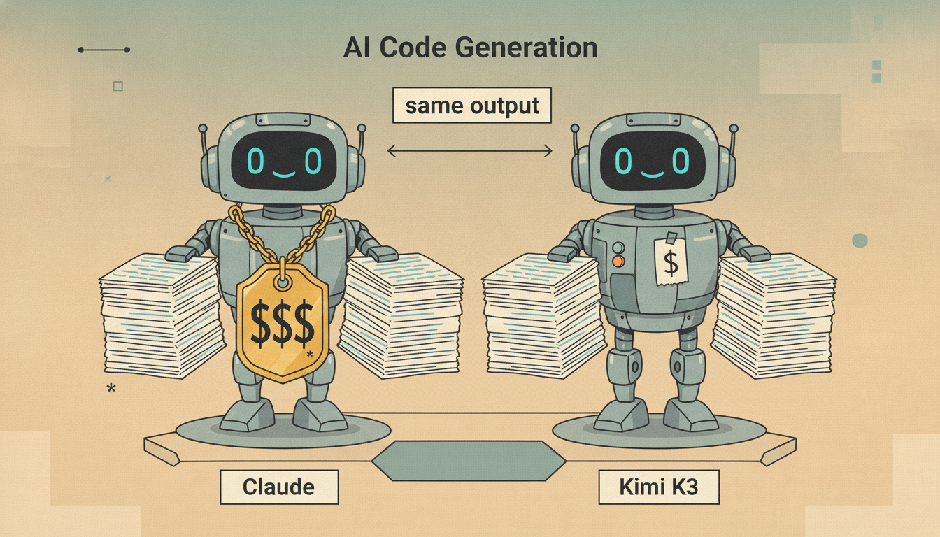
I’ve been running Kimi K3 alongside Claude on my normal coding work, and for all practical purposes I can’t tell them apart. Same tasks, same quality of output, and near identical token counts to get there. I expected an open model to be sloppier or to grind through more tokens on the way to the same answer, and neither turned out to be true.
The prices are nowhere near each other. K3’s API runs $3 per million input tokens and $15 per million output. Claude’s top model costs $10 and $50 for the same units. The subscription side is even more lopsided. Kimi’s paid plans start at $19 a month, and the $39 coding tier is far more generous than anything Claude sells anywhere near that price. Claude’s plans are metered tightly enough that a normal day of agent work can chew through the allowance before lunch.
Then there’s the fine print. Claude couldn’t sustain Fable access on the twenty dollar plan, so they turned it off, and the plan quietly falls back to Opus. When the headline model on your plan can be switched off because the economics don’t work, the plan was never really selling you the headline model. Kimi’s tiers don’t come with that asterisk.
Step back and the bigger story is what an unmitigated failure US AI policy has been. The administration held Fable back, and what finally shipped is a hindered version that refuses whole categories of work. Meanwhile a frontier quality model with none of those restrictions is a download away, released by a Chinese lab the US government has no ability to regulate. Whatever the theory behind gating American models was, it plainly wasn’t thought through, because the only people the gates constrain are American customers. Semgrep found GLM 5.2 beating Claude on their cyber benchmarks for exactly this reason. The restricted model declines the work and the open one just does it.
And it isn’t only Kimi. GLM 5.2 came out under an MIT license, beats the latest Opus release on real work while not even claiming to be frontier, and costs a fraction of it. OpenAI got pushed through the same government gauntlet with GPT-5.6 but came out the other side able to put their flagship on the twenty dollar plan. Whatever you think of OpenAI, they have runway here that Anthropic clearly doesn’t.
I think I can see where this goes. The government will try to regulate AI and open source in particular, and it will run the playbook it ran for the auto industry. Decades of subsidies, bailouts, and protective tariffs produced American carmakers that sell trucks at home and barely register anywhere else in the world. I expect the current administration to reach for the same tools here. Public private partnerships propping up domestic models that only get used inside the US and can’t compete internationally. That’s a sad future where America is the one country without access to the best models at the best prices, buying models deeply tied to the corrupt Trump administration that are neither the highest quality nor the cheapest. Until then, at least, I can’t come up with a reason to keep paying for Claude.
Fable 5 vs. GPT-5.6 Sol on an NP-Hard Problem: Does /goal help?
Fable 5 is an absolute beast; `/goal` is not a game changer.
TL;DR: I gave Claude Fable 5 and GPT-5.6 Sol the same unpublished NP-hard optimization problem, with and without their native /goal mode. Fable 5 is an absolute beast; /goal is not a game changer.
Context: This is an operations research problem originally submitted to students at a hackathon. I spent a week years ago writing C++ to solve it, so I have a useful human baseline.
Fable 5 was an absolute beast on this benchmark. It produced the best solution overall, and its consistency is unlike anything I have seen from a model on this problem. This is pure raw intelligence. Incredible.
The other result is that /goal is not a generic “try harder” switch. It changes the control loop and the search path. Sometimes that finds a better basin. Sometimes it gives a bad idea more time to mature.
All code, prompts, result tables, exclusions, and trajectory notes are in CLIArena. This is a follow-up to my first article about this benchmark.
The problem
KIRO is a fiber-network design problem I worked on as an engineering student in 2018. Given directed distance matrices for Grenoble, Nice, and Paris, the solver has to connect distribution points and terminals using loops and short chains while respecting several structural constraints. The objective is total cable length. Lower is better.
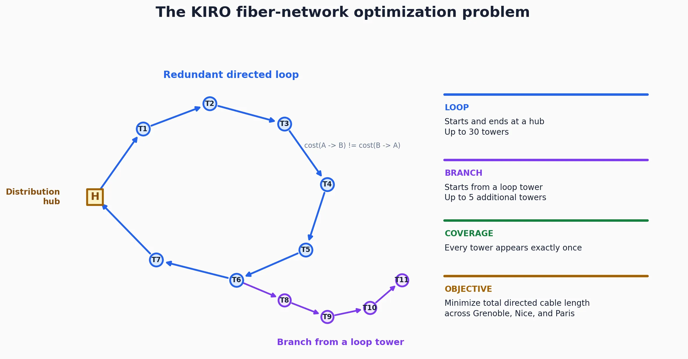
A valid network consists of redundant loops rooted at distribution hubs, with short branches hanging from towers on those loops. Every tower must appear exactly once, and reversing a cable segment can change its cost.
How large is the search space?
There is no single closed-form count because a solution can use any number of loops, variable loop sizes, and differently anchored and ordered branches. But Paris alone gives a useful lower bound.
Even if we ignore ordering and branches and only assign each of the 532 terminals to one of 11 distribution hubs, there are 11^532 possible assignments.
A stronger lower bound comes from one deliberately restricted family of valid solutions: exactly 19 loops of 28 terminals each, with no branches. This covers all 532 terminals because 19 x 28 = 532, while staying below the 30-terminal limit for a loop. Order the 532 terminals, split that ordering into 19 consecutive groups, divide by 19! because the set of loops is unordered, and choose one of the 11 hubs for each loop:
(532! / 19!) x 11^19 ~= 10^1223
What I tested
The primary experiment was intentionally narrow:
| Setting | Value |
|---|---|
| Models | Claude Fable 5, Opus 4.8, Sonnet 5; GPT-5.6 Sol, Terra, Luna |
| Modes | Plain; native /goal |
| Optimization budget | 30 minutes |
| Outer agent timeout | 1,900 seconds |
| Reasoning | Maximum available setting for every model |
| Execution | Harbor 0.1.43, Docker, subscription authentication |
Results
Before concentrating repetitions on the flagship pair, I ran one matched 30-minute no-hint pair for every model in the sweep. For Fable and Sol, the chart uses Pair 1 from the replicated headline set; the other four models have one pair each.
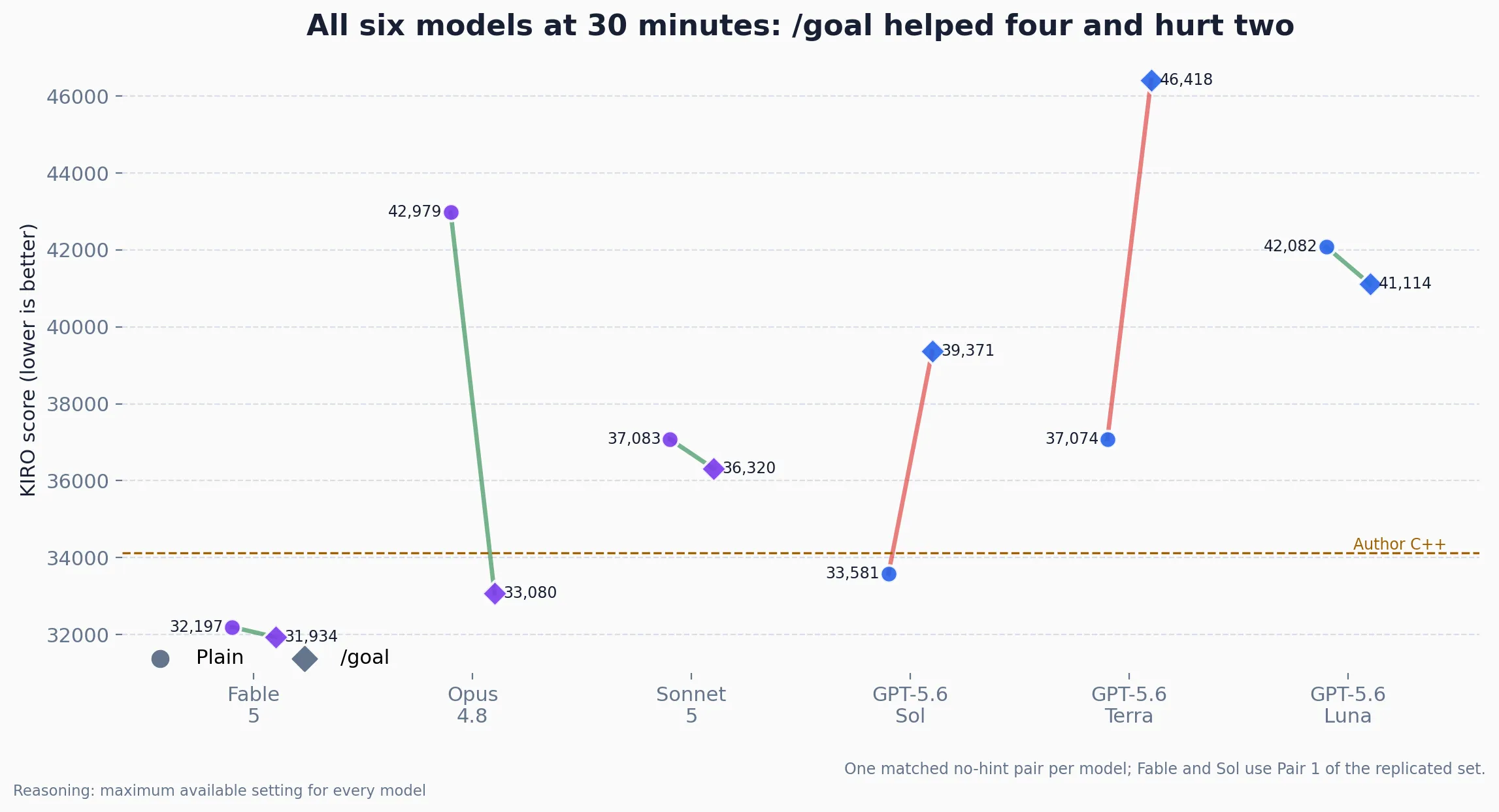
I then repeated the flagship comparison until I had three matched runs for Fable 5 and three for Sol.
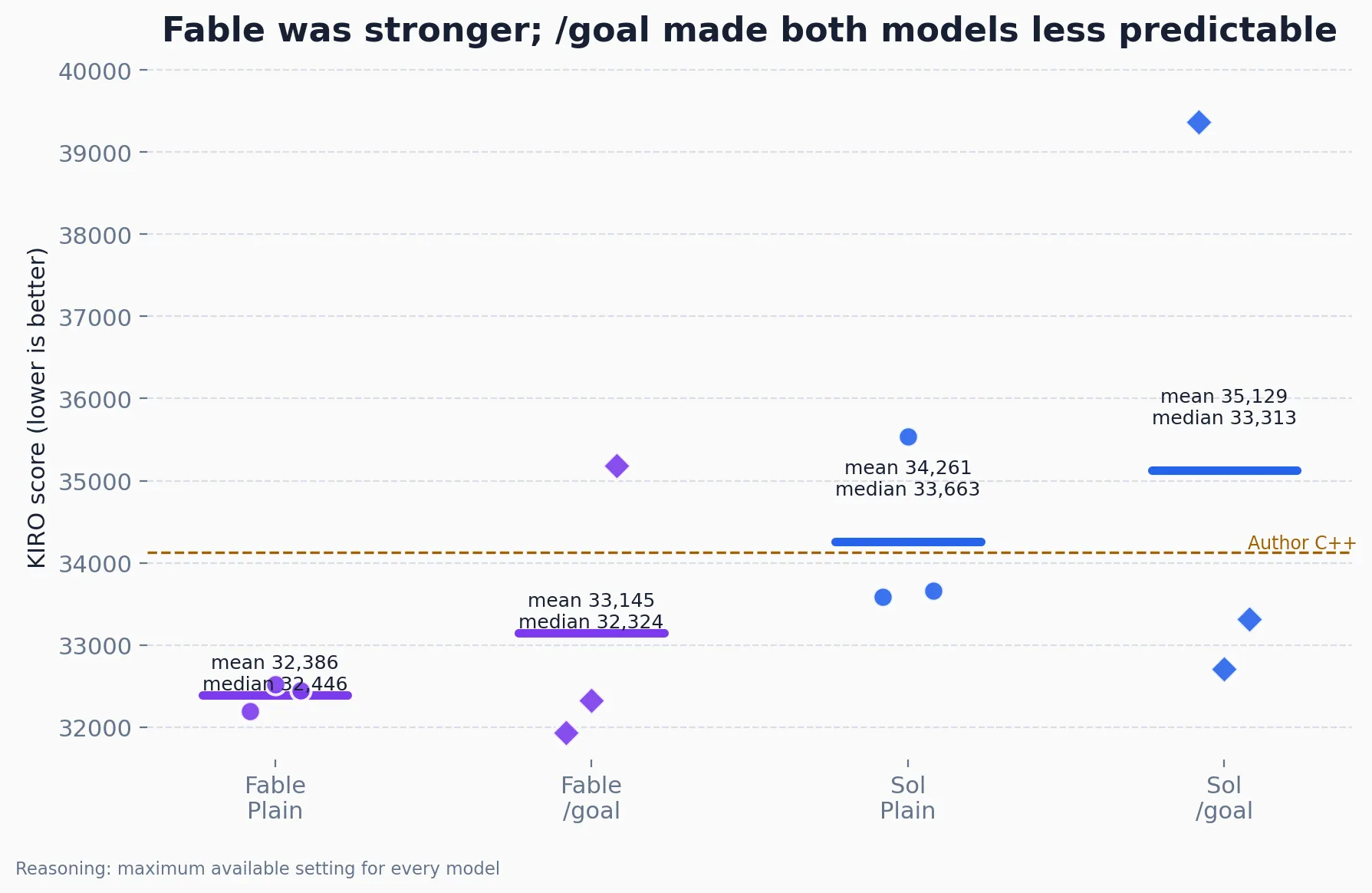
| Model | Run | Plain | /goal |
Goal minus plain |
|---|---|---|---|---|
| Fable 5 | 1 | 32,197 | 31,934 | -263 |
| Fable 5 | 2 | 32,516 | 32,324 | -192 |
| Fable 5 | 3 | 32,446 | 35,178 | +2,732 |
| GPT-5.6 Sol | 1 | 33,581 | 39,371 | +5,790 |
| GPT-5.6 Sol | 2 | 35,539 | 32,703 | -2,836 |
| GPT-5.6 Sol | 3 | 33,663 | 33,313 | -350 |
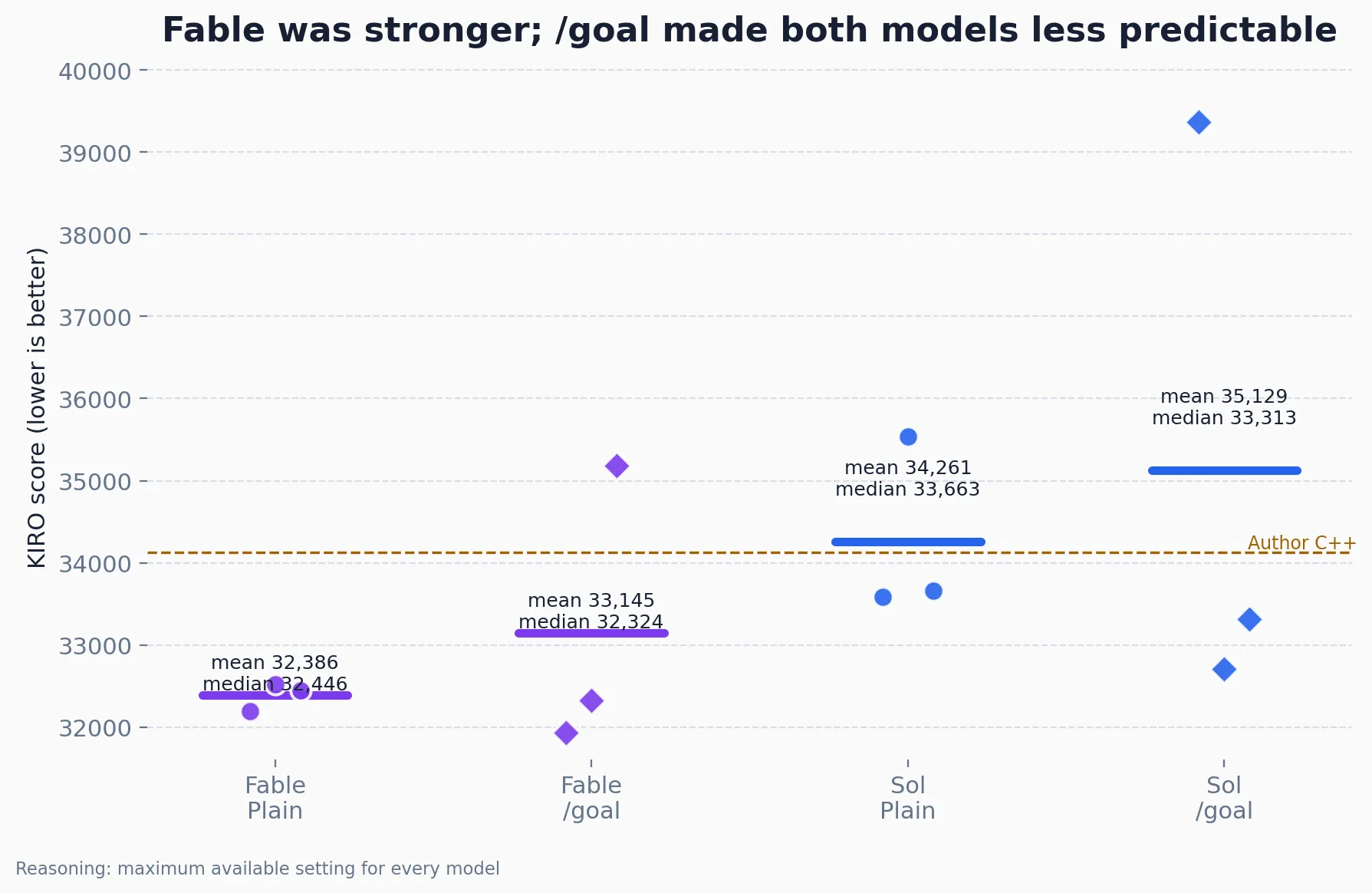
Negative means /goal was better. Goal won four of six trials, so win rate alone makes the feature look useful. The means tell the other half:
| Model | Plain mean | /goal mean |
Mean effect | Median effect |
|---|---|---|---|---|
| Fable 5 | 32,386 | 33,145 | +759 worse | -192 better |
| GPT-5.6 Sol | 34,261 | 35,129 | +868 worse | -350 better |
Both models usually got a small benefit and occasionally suffered a large regression. That is why /goal won most runs but made both means worse.
Fable was also clearly stronger. Its plain mean beat Sol’s by 1,875 points, and its goal mean beat Sol’s by 1,984. More importantly, Fable plain stayed inside a tiny 319-point range while Sol plain spanned 1,958 points. Fable goal produced the best clean score, 31,934; Fable plain was the safest configuration.
Deep dive into the goal command
The same command hides two different systems
Claude Code and Codex both expose /goal, but the implementations are fundamentally different.
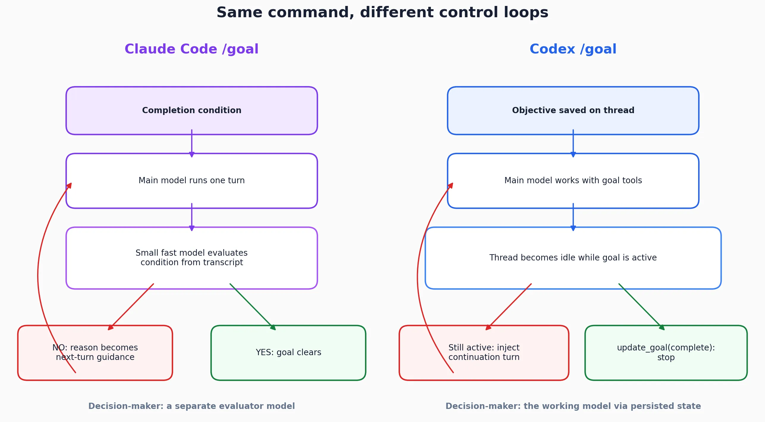
Claude Code: a separate evaluator
Claude Code implements /goal as a session-scoped Stop hook. After each main-model turn, a small evaluator model, Haiku by default, reads the condition and conversation. It returns yes or no with a reason. A no starts another turn; a yes clears the goal.
The evaluator cannot use tools or inspect files. It can only judge evidence that appeared in the transcript. That can catch an early exit, but it cannot know whether another ten million solver iterations are worthwhile. Anthropic’s goal documentation
Keep in mind that claude code is not open source, so we rely solely on what Anthropic tells us.
Codex: persisted state and lifecycle tools
I also read the source for the benchmarked release, Codex CLI 0.144.4. Codex treats a goal as persisted thread state:
- The TUI saves the objective for the active thread, and SQLite stores its status and budget accounting. TUI, schema
- The working model receives
create_goal,get_goal, andupdate_goaltools. Tool specification - If the thread becomes idle while the goal is active, Codex injects a continuation turn with the objective and a completion audit. Runtime, prompt
Claude delegates completion to another model. Codex lets the working model declare completion, then resumes it while the persisted goal remains active. Claude’s evaluator is independent but sees only the transcript; Codex sees the files and tools but effectively grades its own work.
Why /goal can win most runs and still be a bad default
On a normal coding task, progress is often legible: another turn can fix a test or complete a migration. Optimization is different. Once an agent chooses a solver, extra time can amplify either a good decision or a bad one.
That is exactly what happened here. Goal helped when it sustained Fable’s fast compiled portfolio or Sol’s successful chain repartition. It hurt when Fable built a slow solver or Sol committed to an exhaustive anchor sweep. The median moved slightly in the right direction; the bad tail moved much farther in the wrong one.
Limitations
This is one unpublished NP-hard task, not a general coding leaderboard. Only Fable and Sol have three clean matched pairs. Other comparisons mix prompts, wrapper versions, and time limits, and the trials ran sequentially through subscription services that may have drifted.
The containers exposed eight CPUs despite task metadata declaring one, which favored Fable’s parallel portfolios. Every scored Fable and Sol output was valid, partly because the wrapper required early checkpoints and final verification. The benchmark measures the complete system: model, CLI, prompt, subscription service, and harness.
Reproducing this
The benchmark task, wrappers, analysis scripts, figure generator, and full evidence memo are in CLIArena. Raw job directories are excluded from Git because of their size, but the memo records every publishable score, city breakdown, elapsed time, strategy, exclusion, and run ID.
The primary commands are:
RUN_ID=article-kiro-YYYYMMDD-clean \
PHASE=nohint-all \
./scripts/run_subscription_article_matrix.sh

uv run python scripts/summarize_subscription_article_results.py RUN_ID...
uv run python scripts/analyze_subscription_article_results.py RUN_ID...
The result I would put in the headline is not that goal helps or hurts. It is that a persistence feature can win most individual trials while making observed average performance worse. On a hard optimization problem, the quality of the loop matters less than the quality of what the loop keeps doing.
Setting up your spare Mac for Claude Code to control, a step-by-step guide
Turn your spare Mac into an always-on machine Claude Code can fully control.
Here’s a full step-by-step guide on how to turn your spare Mac into an always-on machine Claude Code can fully control, with computer use enabled. You’ll be able to talk to it from your phone through the Claude app, or from your main Mac over SSH.
In case you’re reading this on GitHub Pages, here’s the repo version.
Why do this?
I wanted to create a separate environment Claude Code can control on its own, so I can delegate tasks I don’t necessarily want to run on my own machine - certain types of research tasks, and development tasks.
Claude Code, especially with the --dangerously-skip-permissions flag on, carries inherent risk when run on your main machine. You can eliminate / mitigate these risks by creating a separate environment on your spare Mac with everything it needs to have access to.
It has an added bonus of being able to talk to Claude Code anytime, anywhere from your phone. I’ve personally found it really useful because I often prefer to talk to Claude Code instead of regular Claude on the mobile app - Claude Code is often more capable.
The following guide assumes you have your main Mac as well as a spare Mac you can set up for this, but you should be able to take inspiration from it and apply it to any combination of two machines.
Why this setup?
First, let’s quickly address a few questions you might have.
Why not run it in a container?
I’m a big proponent of running it in a container - I even built an entire environment for doing so conveniently. However, I’ve found it has a few limitations. First, it still runs on your main machine, so it’s not completely separated. For example, network requests it sends still go through your main machine.
Second, there are limitations to the container’s capabilities. For example, I wanted my agent to be able to run Unity for game development, and there’s no easy way to do that in a container. The same goes for any other app that’s only available on a Mac - you won’t have access to it. That’s especially relevant if you want Claude Code to control these apps through computer use - clicking, dragging, and so on.
Why not use something like OpenClaw?
I personally like having access to the full, latest features of Claude Code. I also like being able to control it from the Claude app - I’ve found it really convenient. And you get to use your Claude subscription usage if you happen to have one, which is an added bonus.
At the end of the day, running an agent with broad permissions is safer on a machine that has nothing to lose - but you get the benefit of being able to use a full Mac instead of a container. The approach here:
- Use an old/spare Mac, not your main one.
- Create a fresh local account with no personal data and no Apple ID signed in, so the agent has nothing sensitive to reach.
- Drive it over SSH from your main Mac on your local network, and control it from your phone.
1. Start fresh on the target Mac
Wipe it first (if it has any personal data)
You’ll be giving the agent full access to this machine, so it can reach anything stored on it. If there’s existing data you don’t want it to have access to, erase the machine first:
- Macs that support it: System Settings -> General -> Transfer or Reset -> Erase All Content and Settings.
- Older Intel Macs: restart into Recovery (hold Cmd-R at boot), use Disk Utility to erase the internal drive, then reinstall macOS.
Optionally update to the latest macOS afterward (System Settings -> General -> Software Update).
Create a fresh, isolated account
- Create a new local user account (System Settings -> Users & Groups).
- I recommend not signing into an Apple ID. Skip it during setup.
Make the account an admin (if you haven’t already)
The account needs admin rights or sudo will refuse to run.
- System Settings -> Users & Groups -> set the account to Allow this user to administer this computer.
- If you ever need to repair it from another admin account:
sudo dseditgroup -o edit -a <user> -t user admin
2. Enable Remote Login (SSH) on the target Mac
On the target, turn on SSH so the source Mac can connect:
sudo systemsetup -setremotelogin on
If the command fails with Turning Remote Login on or off requires Full Disk Access privileges, give your terminal app Full Disk Access first:
- System Settings -> Privacy & Security -> Full Disk Access.
- Click +, then in the file picker go to Applications -> Utilities -> Terminal and add it.
- Quit and reopen the terminal, then rerun the command.
3. Passwordless sudo for the target account
This is so the agent (and your SSH commands) can run admin tasks without a password prompt each time. Run this once on the target. It asks for the login password this one time:
echo "<user> ALL=(ALL) NOPASSWD: ALL" | sudo tee /etc/sudoers.d/<user>-nopasswd >/dev/null
sudo chmod 440 /etc/sudoers.d/<user>-nopasswd
sudo visudo -cf /etc/sudoers.d/<user>-nopasswd   # validate - must print 'parsed OK'
This creates a small rule file telling the Mac that <user> can run sudo without a password prompt:
- line 1 writes the rule into
/etc/sudoers.d/. - line 2 makes it read-only - sudo ignores the file otherwise.
- line 3 validates the syntax; a typo in a sudoers file can lock you out of
sudoentirely, so it must printparsed OK.
After this, sudo runs with no prompt - test with sudo -n true, which succeeds silently if passwordless sudo works.
4. Find the target’s address (hostname or IP)
You can reach the target by either a hostname or an IP. I recommend using the hostname: it stays the same, while the IP can change.
Hostname (recommended). Run on the target:
scutil --get LocalHostName # prints the hostname, e.g. MacBook-Pro
Add .local to form the address: <target-host>.local. You can also read it from System Settings -> General -> Sharing, shown as Local hostname.
Give the target a unique name. Each Mac needs a
.localname that’s unique on your network. If two machines share a name, the address can point to the wrong Mac. Make sure the target’s name is unique - rename it if needed:sudo scutil --set LocalHostName newmacbook # -> newmacbook.local
IP address (not recommended). Run on the target:
ipconfig getifaddr en0 # e.g. 192.168.1.80
Note that the IP can change after a reboot or after a certain amount of time.
Throughout the rest of this guide, replace <user> with the target account name and <target-host> with the hostname from above, so the address is <user>@<target-host>.local. You could also instead use an IP in place of <target-host>.local.
5. Set up passwordless SSH from the source Mac
On the source Mac, create an SSH key (skip if you already have one):
ssh-keygen -t ed25519
Install your public key on the target. This asks for the target account’s login password once:
ssh-copy-id <user>@<target-host>.local
Test it - this should print the target username with no password prompt:
ssh <user>@<target-host>.local whoami
6. Keep the target awake
By default macOS sleeps after ~10 minutes idle, even when plugged in, which takes it off the network. To make it never sleep, run this on the target (or over SSH from the source):
sudo pmset -c sleep 0          # never system-sleep while plugged in (-c = on charger)
sudo pmset -c disablesleep 1   # also prevents sleep with the lid closed (clamshell)
sudo pmset -c displaysleep 0   # keep the display on too
Verify:
pmset -g | grep -iE 'sleep'
sleep 0, SleepDisabled 1, and displaysleep 0 in the output confirm it worked.
If the machine runs on battery sometimes, use -a instead of -c to apply to all power sources (at the cost of battery drain).
The screen can still lock when the screen saver kicks in. Stop the screen saver from ever starting so it never locks on its own:
defaults -currentHost write com.apple.screensaver idleTime 0
7. Clipboard sync over SSH
macOS ships pbcopy (write clipboard) and pbpaste (read clipboard). Piped over SSH, they can move the clipboard between machines - encrypted, peer-to-peer, no Apple ID or third-party service.
clip.sh wraps this into one command with two subcommands, and adds image support on top of pbcopy/pbpaste (which are text-only). Install it as a script on your PATH on the source Mac, and point it at the target host with IC_BOX (“ic” standing for “isolated claude”):
curl -fsSL https://raw.githubusercontent.com/ykdojo/claude-controls-mac/main/clip.sh -o ~/.local/bin/clip
chmod +x ~/.local/bin/clip
export IC_BOX="<user>@<target-host>.local"   # add to ~/.zshrc
Usage:
clip send- this Mac’s clipboard → the target (text or image). For an image you can paste it straight into a Claude Code session on the target with Ctrl-V.clip get- the target’s clipboard → this Mac (text or image).
8. Install Claude Code on the target Mac
Send the install command over and run it. From the source Mac you can push it straight to the target’s clipboard, or run it remotely. The following command installs a specific version, but you can also install latest or stable if you’d like:
ssh <user>@<target-host>.local 'curl -fsSL https://claude.ai/install.sh | bash -s -- 2.1.201'
The native installer may warn that ~/.local/bin is not on PATH. Fix it on the target by adding it to ~/.zshenv (not ~/.zshrc) - .zshenv is read by every zsh, including non-interactive ones:
ssh <user>@<target-host>.local 'echo '\''export PATH="$HOME/.local/bin:$PATH"'\'' >> ~/.zshenv'
9. Set up an opinionated, Claude Code-friendly environment (optional)
This optional step applies a set of opinionated defaults via setup-claude-env.sh - shell aliases, the DX plugin, settings.json tweaks, the GitHub CLI, and (opt-in) Playwright MCP and yt-dlp. Every item is toggleable; see the full list in claude-env-components.md.
Interactively on the target - shows a checklist of every item (core pre-checked, opt-ins unchecked) so you can pick any combination. Download the script onto the target and run it:
ssh -t <user>@<target-host>.local \
  'curl -fsSL https://raw.githubusercontent.com/ykdojo/claude-controls-mac/main/setup-claude-env.sh -o setup-claude-env.sh && bash setup-claude-env.sh'
Non-interactively - the script goes into this mode if it detects a non-interactive environment or you supply at least one flag. No prompt; installs core only by default, or pick what you want with flags (--yt-dlp, --playwright, --all, --core):
ssh <user>@<target-host>.local \
  'curl -fsSL https://raw.githubusercontent.com/ykdojo/claude-controls-mac/main/setup-claude-env.sh -o setup-claude-env.sh && bash setup-claude-env.sh --all'
The script is idempotent (OK to re-run).
10. Log in to Claude and GitHub
Both logins are interactive, so SSH in:
ssh <user>@<target-host>.local
Then run claude on the target - it drops into the login for your Anthropic account. Follow the prompts (a browser/device-code flow you can finish from a browser on your main Mac).
GitHub - optional, but highly recommended so the agent can work with repos:
gh auth login
If you haven’t installed the GitHub CLI from the previous step, make sure to do so first.
I personally recommend using a separate GitHub account, not your main one, so it doesn’t mess up your main account.
11. Computer use over SSH (optional)
This lets an interactive claude session on the target see (screenshots) and control (mouse/keyboard) its own desktop, driven over SSH.
This doesn’t work out of the box - SSH and macOS’s permission model get in the way, so the setup below exists to route around that.
Why it needs a workaround: macOS gates screen capture and input behind Screen Recording and Accessibility permissions that are tied to the GUI login session, so an SSH process can’t reach the display. Fix: a LaunchAgent keeps a tmux server alive inside the GUI session on a fixed socket; every claude session created there lands on that server and inherits the GUI session, so it can reach the display. You attach over SSH.
Scriptable setup
Run setup-computer-use.sh on the target:
ssh -t <user>@<target-host>.local \
  'curl -fsSL https://raw.githubusercontent.com/ykdojo/claude-controls-mac/main/setup-computer-use.sh -o setup-computer-use.sh && bash setup-computer-use.sh'
This installs the LaunchAgent (persistent tmux server with anchor session cc) and enables the built-in computer-use tool in ~/.claude.json. Requires tmux (brew install tmux) and a Claude Pro or Max plan. Re-runnable; --uninstall to remove.
Use it from your Mac
Install ic.sh (ic = “isolated claude”) on the source Mac:
curl -fsSL https://raw.githubusercontent.com/ykdojo/claude-controls-mac/main/ic.sh -o ~/.local/bin/ic
chmod +x ~/.local/bin/ic
echo 'export IC_BOX="<user>@<target-host>.local"' >> ~/.zshrc   # or edit the default in the script
Each ic spawns its own claude session on the box (run several at once) and attaches. Flags mirror claude, and it adds several more subcommands:
ic               # new claude session
ic -c            # continue the most recent conversation (forwards to: claude -c)
ic -r            # resume picker (forwards to: claude -r)
ic --chrome      # with Claude in Chrome (forwards to: claude --chrome)
ic sh            # a plain shell on the box, no claude (alias: ic shell)
ic vnc           # open Screen Sharing (VNC) to the box (see step 15)
ic rc            # Remote Control: drive the box from your phone (claude remote-control)
ic history       # stored conversations: count, location, recent w/ previews (alias: hist)
ic ls            # list live sessions (state, age, what's running, conversation)
ic attach <id>   # attach a running session (alias: ic a)
ic kill <id>     # kill a session (alias: ic k)
ic kill-all      # kill all sessions
ic kill-except <id> <id> ...   # kill all sessions except the listed ones
ic -h            # help
All ic sessions run with --dangerously-skip-permissions (and ic rc uses --permission-mode bypassPermissions).
Copying text out: sessions run in tmux, and Terminal.app can’t receive the clipboard escape sequences (OSC52) that claude emits, so mouse-selecting a snippet won’t reliably reach your Mac clipboard. Quick workaround: Cmd-A then Cmd-C copies the whole visible screen.
Bonus: let your Mac’s Claude drive the box’s Claude
Because every ic session lives on the box’s tmux server at a fixed socket, a Claude Code session on your source Mac can prompt one directly over SSH - useful for delegating work to the box and checking on it, agent to agent:
# find the session (ic ls prints the ids)
ic ls

# type a prompt into it, then confirm with a second Enter - with longer prompts,
# an Enter sent in the same burst as the text doesn't register as submit and the
# prompt sits in the input box (short prompts usually submit fine)
ssh <user>@<target-host>.local "tmux -S /tmp/cc-tmux.sock send-keys -t <session> 'Switch to main and pull; PR #4 is merged.' Enter"
sleep 2
ssh <user>@<target-host>.local "tmux -S /tmp/cc-tmux.sock send-keys -t <session> Enter"

# read the reply (re-run / poll until the spinner is gone)
ssh <user>@<target-host>.local "tmux -S /tmp/cc-tmux.sock capture-pane -t <session> -p" | tail -30
One-time grants (can’t be scripted)
Screen Recording and Accessibility can only be granted in the GUI, and a human has to do it at the machine (in person or via Screen Sharing) - macOS blocks synthetic clicks on these prompts. On first capture you’ll also Allow a “bypass the window picker” prompt (recurs ~monthly).
The grants go on tmux, not claude. macOS attributes capture/control to the responsible process in the chain, which here is the tmux server (claude runs as its child). So:
- Grant
tmux(/usr/local/bin/tmux, or/opt/homebrew/bin/tmuxon Apple Silicon) under both Screen Recording and Accessibility - Screen Recording covers screenshots, Accessibility covers mouse/keyboard control. - Restart the tmux server after granting - a running process caches its permission state at launch, so a grant won’t take effect until the server restarts:
tmux -S /tmp/cc-tmux.sock kill-server(the LaunchAgent respawns the anchor within seconds). claude sessions started after the restart pick up the new grant.
To make the entries appear in System Settings in the first place, trigger a computer-use action (ic, then ask Claude to “take a screenshot”) - macOS adds tmux to the list (toggled off) so you can switch it on.
Full Disk Access stops the “access data from other apps” prompts. On newer macOS, tmux triggers a separate “tmux would like to access data from other apps” prompt for each app whose data anything inside it touches. Granting tmux Full Disk Access (same Privacy & Security pane) suppresses these prompts entirely: use the + button and add the tmux binary (Cmd-Shift-G to type the path). Restart the tmux server afterward, as above.
12. Install a VPN, or any other app (optional)
I personally like to run a VPN on the box so its traffic goes out separately from my local IP. I use Proton VPN - it has a free option and I’ve been using them for a long time - but of course there are other options.
You can just ask the box’s Claude to do it if you finished walking through the previous step: ic in and say “install Proton VPN”. It’ll download and install the app. The parts it can’t do alone:
- Credentials. Signing in is required even for the free tier, and that’s yours to enter. Send the password over securely with
clip sendfrom step 7: copy it on your Mac, runclip send, then paste into the sign-in field on the box. - macOS permission prompts. The first connect pops a system prompt to allow a VPN / network configuration (and may ask for the Mac password) - approve it at the machine.
- Computer use for the GUI. The app is GUI-only, so driving it relies on step 11 being set up. Once signed in, the agent can connect and switch servers itself.
This general flow works not just for a VPN app - it should work for pretty much any other application too.
13. Control it from your phone
Remote Control lets you drive Claude Code from your phone through the Claude app. There are two ways to use it:
- Run
/remote-control(or/rcfor short) inside an existing session and follow the instructions - you can then drive that same session from your phone, going back and forth between the two. - Start a server with
claude remote-control, which also lets you start brand new sessions from your phone, not just attach to one you already have open.
If you went through step 11, ic rc starts that server for you in a way that the sessions you spawn from your phone have access to computer use too.
14. Set up Claude in Chrome (optional)
Computer use from step 11 deliberately won’t control a browser - browsers get a restricted tier where Claude can see what’s on screen but can’t click or type in it. The Claude in Chrome extension fills that gap with proper browser control: navigating, clicking, filling forms, reading console logs and network requests. And unlike Playwright MCP, it drives your regular Chrome profile, so the agent can use any logged-in state you set up on the box.
It requires Chrome on the target and a direct Anthropic plan (Pro, Max, Team, or Enterprise).
You can ask the box’s Claude to install Chrome and open the extension’s Chrome Web Store page. The parts it can’t do alone (do these at the machine, in person or via Screen Sharing):
- Click “Add to Chrome”. Optionally, you can pin the extension to the toolbar by going to
chrome://extensions. - Log into your Claude account in the extension. You can send the login info with
clip sendfrom step 7.
Then enable it in Claude Code on the target: run /chrome in a session and select “Enabled by default” to have the browser tools in every session, or skip that and use claude --chrome per session (ic --chrome from your source Mac). If the connection doesn’t work, try restarting Chrome once.
To make browser use efficient (element refs from the accessibility tree instead of coordinates, no unrequested screenshots), the environment setup from step 9 adds a “Claude for Chrome” guidance section to ~/.claude/CLAUDE.md on the target. If you skipped that step, re-run the script - it’s idempotent.
If your source Mac’s Chrome also has the extension signed into the same account, Claude Code can connect to either browser. It prompts you to pick when both are connected, but its local-machine detection can be wrong (#74667). To avoid that, you can temporarily uninstall the extension from the source Mac’s Chrome - or just quit Chrome on the source while the box is working.
Note that sessions spawned from your phone via step 13 don’t currently get the browser tools (#74671) - the workaround is to start the session in the terminal and attach with /rc.
15. Enable Screen Sharing on the target Mac (optional)
This lets you see the target’s screen live from the source Mac - and take over its mouse and keyboard - using macOS’s built-in Screen Sharing.
This has to be enabled in the GUI at the machine - since macOS 12.1 it can’t be enabled from the command line.
On the target: System Settings -> General -> Sharing -> Screen Sharing on. If Remote Management is on, the Screen Sharing toggle may be hidden - turn it off first.
Then connect from the source Mac:
open vnc://<user>@<target-host>.local
Log in with the target account’s login password and tick Remember this password in my keychain.
16. Access it from anywhere with Tailscale (optional)
.local names only resolve on your LAN, so everything so far is local-network only (except phone control from step 13, which relays through Anthropic). Tailscale fixes that: it connects your machines with peer-to-peer, end-to-end encrypted WireGuard tunnels, so SSH, ic, clip, and Screen Sharing work from any network with nothing exposed to the public internet. On your home network it takes a direct LAN path, so local use stays as fast as before. And joining the network only gives a device reachability - SSH and Screen Sharing still require your key or password on top.
Install on the target (the Homebrew formula works headless over SSH; sign in at the URL the last command prints - a free account with a social login is fine):
ssh <user>@<target-host>.local 'brew install tailscale'
ssh <user>@<target-host>.local 'sudo brew services start tailscale'
ssh <user>@<target-host>.local 'sudo tailscale up --operator=<user>'
Install on the source, then open the Tailscale app and log in with the same account - devices only see each other within one account’s network:
brew install --cask tailscale-app
With MagicDNS (on by default) the target is reachable by bare hostname from anywhere - the same address, minus .local. Switch IC_BOX in ~/.zshrc, keeping the original name for reference:
export IC_BOX="<user>@<target-host>"          # Tailscale - works remotely too
# export IC_BOX="<user>@<target-host>.local"  # original - local network only
Screen Sharing works the same way: open vnc://<user>@<target-host>.
Recommended, in the admin console: device approval (Settings -> Device management), so a compromised Tailscale login alone can’t add a device to your network, and disable key expiry on the target (Machines -> …), so the box doesn’t drop off the network when its key expires after ~180 days.
To confirm remote access really works, put the source Mac on a different network (e.g. a phone hotspot) and run ic ls.
Why do AI company logos look like buttholes? (2025)
If you ever thought that AI company logos look like buttholes, you're not alone.

If you pay attention to AI company branding, you'll notice a pattern:
- Circular shape (often with a gradient)
- Central opening or focal point
- Radiating elements from the center
- Soft, organic curves
Sound familiar? It should, because it's also an apt description of... well, you know.
A butthole.
The circular AI logo epidemic
If you ever thought that AI company logos look like buttholes, you're not alone.
FastCompany noticed this trend in 2023 and published an article about it, but (I could only presume) their editors and lawyers didn't let them title the article the way the wanted it to title, so it got published with a more safe for work title: The AI boom is creating a new logo trend: the swirling hexagon. They also were careful not to mention anything anatomical.
I don't have editors or lawyers, so let's take a closer look at some examples:
OpenAI's logo evolution

OpenAI's original logo was a simple, text-based mark. Then came the redesign: a perfect circle with a subtle gradient and central void.
OpenAI's official explanation is a masterclass in corporate euphemism:
"The Blossom logo is more than just a visual symbol; it represents the core philosophy that guides our approach to design and innovation. At its heart, the logo captures the dynamic intersection between humanity and technology—two forces that shape our world and inspire our work. The design embodies the fluidity and warmth of human-centered thinking through the use of circles, while right angles introduce the precision and structure that technology demands."
Sure, Sam.
Translation: "We made a circular shape with some angles because it looked nice, then wrote flowery language to justify why our butthole-adjacent design is actually profound."
The fluidity and warmth of human-centered thinking through the use of circles is perhaps the most elegant way anyone has ever described making a logo that resembles an anus.
The Big AI companies
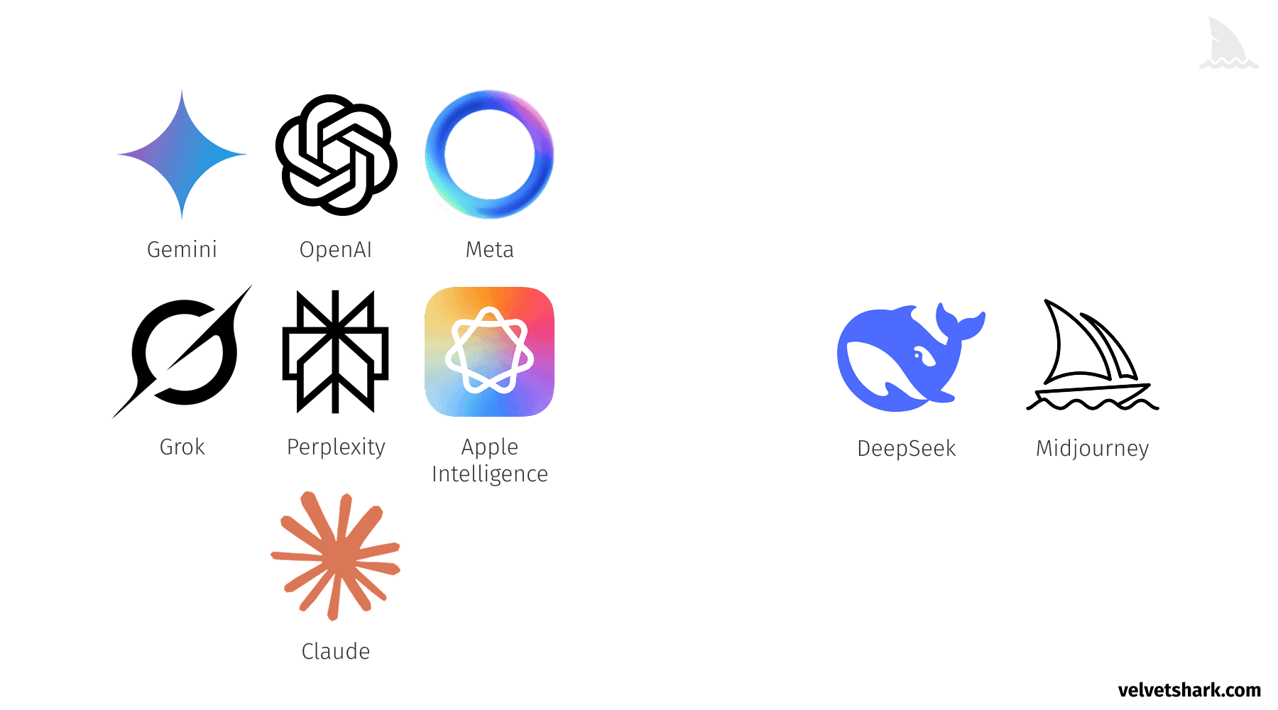
Looking at the logos of the Big AI companies, you can see that they almost all of them have a circular or snowflake-like shape and a central opening.
Only DeepSeek and Midjourney don't follow the trend. Interestingly, both are sea-related.
Smoking gun: Anthropic's Claude
Up until this point, the logos have been subtle. You might say that the logos are simply circular and there's not much more to it.
But Anthropic's Claude takes it to the next level.
Here's a side-by-side comparison with a drawing from Kurt Vonnegut's book "Breakfast of Champions". I added Claude's logo below for easy comparison.

Both the drawing and the description in the book are unambiguous. This is not just "a circular shape with a gradient" anymore, is it?
July 2026 update: the smoking gun now moves
Since publishing this article, I've discovered new evidence. Open claude.ai and click on the Claude logo. Just watch what it does:
The Claude logo, when clicked. I have no further questions.
Every click makes the logo clench and relax. It even responds with a slightly annoyed "Yes, yes. What can I do for you?", as if you poked something you weren't supposed to.
At this point, there's no argument you could make that would persuade me this is not a butthole 🙂
It's not just AI companies
Even traditional companies aren't immune. Here are a few notable or funny examples. But the percentage of AI company logos that look like buttholes is still significantly higher than than any other industry.

I especially like the Electrolux one. It's simple, memorable, and once you see a butt and bikini, you can't unsee it.
Why does this keep happening?
There are several factors at play:
Circular design psychology
Circles represent wholeness, completion, and infinity—concepts that align with AI's promise. They're also friendly and non-threatening, qualities companies desperately want to project when selling potentially job-replacing technology.
Unintentional biomimicry
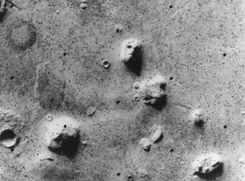
The human brain finds familiar patterns in random shapes (pareidolia), like a face on Mars, taken by the Viking 1 orbiter and released by NASA in 1976.
But sometimes, designers inadvertently recreate biological forms without realizing the... anatomical implications.
The copycat effect
Once a few major players adopted the circular sphincter aesthetic, everyone followed suit. Now we have an industry where standing out means looking exactly like everyone else's butthole.
Basically, the same reason why so many brands change their logos and look like everyone else.
Tech and fashion logos using sans serif fonts
Design by committee
Another factor is how these logos are created. Important corporate decisions involve many stakeholders. The result is often the safest, most inoffensive option, the average of everyone's opinions. In design meetings at AI companies, conversations probably sound like:
- Can we make it more futuristic?
- It needs to feel advanced but approachable.
- Let's add a subtle gradient to convey intelligence.
No single person suggests making a logo that resembles an anus, but when everyone's feedback gets incorporated, that's what often emerges. Risk aversion in corporate environments naturally pushes designs toward familiar, "safe" territory, which apparently means anatomical openings.
What this says about tech branding
This phenomenon reveals something deeper about the tech industry: the fear of standing out too much. Despite claims of innovation and disruption, there's tremendous pressure to look legitimate by conforming to established visual language.
When OpenAI's sphincter-like logo became successful, it created a template that said, "This is what serious AI looks like." Now, any new AI company that doesn't resemble a colorful anatomical opening risks being seen as unserious or unprofessional.
Tech design trends through history
This isn't the first time tech design has gone through a conformity phase. Consider these previous waves:
- 1990s-2000s: 3D and Glossy - Remember when every logo needed a drop shadow and a glassy shine? Apple's aqua interface set the standard.
- 2010-2013: Skeuomorphism - Digital designs mimicking physical objects, with stitched leather textures and realistic dials.
- 2013-2018: Flat Design - Reaction to skeuomorphism brought minimal, clean interfaces with bright colors and no shadows.
- 2018-2022: Neomorphism - Soft shadows and semi-flat design creating subtle, "touchable" interfaces.
- 2022-Present: The Butthole Era - Circular gradients with central focal points dominating AI branding.
Each era started with innovations that were quickly copied until the industry reached saturation point and moved on to the next trend.
Sans serif bags
Logos become increasingly interchangeable (one of the bags is real, but they all look the same)
Historic logo disasters: You're not alone
AI companies can take some comfort in knowing they're not the first to face unintended anatomical comparisons. Logo history is filled with disasters but to keep this consistent with the theme of the article, here's a couple of them.
Logo disasters
- Zune logo, when flipped, says something different. Maybe that's one of the reasons why iPod won?
- Brazilian Institute of Oriental Studies is a stylized pagoda silhouetted against the setting sun. Or so the designers wanted it to look. The final result was much more... anatomical. They since changed it to something less suggestive.
Maybe companies should have a panel of "middle schoolers" on their payroll to review logos before launch. They'll find every possible inappropriate interpretation with ruthless efficiency.
Breaking free from the butthole
For companies brave enough to differentiate, here are some alternatives:
- Embrace sharp angles - geometric shapes with defined edges create a distinct visual identity
- Use negative space creatively - think FedEx arrow, not biological openings
- Avoid radial symmetry - not everything needs to be perfectly circular
- Skip the gradient - flat design still works
- Test with diverse audiences - if five different people independently say "that looks like a butthole," it probably does (show it to teenagers if you want to uncover even the most subtle anatomical implications)
Conclusion
Does this mean AI companies should change their branding? Not necessarily. The familiarity clearly works in building trust. But perhaps the next wave of AI innovation could be accompanied by some visual innovation too.
For companies looking to break the mold, consider these approaches that successful tech brands have used:
- Embrace meaningful abstraction - Slack's hashtag-inspired logo communicates collaboration without circular clichés
- Leverage letterforms - Netflix's simple "N" has become instantly recognizable without anatomical confusion
- Tell a story - Stripe's distinctive parallel lines reflect payment flows moving seamlessly
- Use distinctive color combinations - Twitch's purple branding stands out in a sea of blue tech logos
The challenge for the next generation of AI companies isn't just technological - it's finding visual language that communicates innovation without resorting to the same tired sphincter-inspired patterns.
PS. This post is meant to be humorous, but let's not pretend there isn't a serious point here about the depressing sameness in modern design. No actual anuses were consulted during this research, though several designers were clearly thinking about them.
TP-Link Kasa cameras leaked home GPS via unauthenticated UDP for 6 years
★ 15⑂ 0 forks
Python
Independent IoT security research, vulnerability disclosures, and PoCs focusing on firmware analysis, hardware interfaces, and cryptographic flaws.
Qubes OS Security in the Public Record
Abstract:Qubes OS is a revealing case for security measurement because its architecture makes component boundaries security-relevant. We present a protocol-driven longitudinal analysis of 109 public Qubes Security Bulletins (QSBs, 2011--2025), the official Qubes-maintained Xen Security Advisory (XSA) tracker, and a secondary vulnerability-event sensitivity series. The study measures the public advisory record rather than latent vulnerability incidence or realized compromise. The methodology combines audited deterministic component attribution, change-point analysis, overdispersion checks, severity-proxy weighting, censoring sensitivity, documentary latency lower bounds, and baseline-aware evaluation of vulnerability discovery models (VDMs).
The results show persistent upstream dependence in that public record. On the official tracker, 113 of 464 XSAs affect Qubes; under primary labeling, 87 of 109 QSBs (79.8\%) are attributable to Xen, CPU/microarchitectural, or other upstream components rather than Qubes-core logic, with similar results under weighted views. Change-point analyses identify 2015Q1 as the dominant break in the quarterly advisory series, while post-2018 annual disclosure rates are statistically flat. Poisson inferences are stable under dispersion diagnostics and negative-binomial sensitivity checks. The attribution codebook performs well in a stratified 30-QSB audit, and S-shaped VDMs fit descriptively but do not significantly outperform a rolling-mean baseline in short-horizon forecasts.
Overall, the Qubes public advisory record appears stable, but not quiet: disclosure activity plateaus at a higher level than in the earliest years, while the observed burden remains concentrated in upstream trust anchors.
In-toto: A framework to secure the integrity of software supply chains
Speech Recognition and TTS in less than 500kb
★ 9,048⑂ 487 forks
C++
Very low latency speech to text, intent recognition, and text to speech, for building voice agents and interfaces

Moonshine Micro — Voice Interfaces for Microcontrollers
Moonshine Voice is an open source AI toolkit for developers building real-time voice agents and applications. Moonshine Micro is a version designed specifically for embedded system processors like microcontrollers and DSPs, and uses the Raspberry Pi RP2350, which retails for just 80 cents, as its reference platform. It includes voice-activity detection, command recognition, and neural speech synthesis and can run in as little as 470 KB of RAM.
You can see a full walkthrough in the video below:

The memory and compute requirements are designed to fit resource-constrained systems. Figures below are for the RP2350 demo; the detailed memory budget breaks each one down:
| Component | Flash | SRAM (arena peak) | Compute |
|---|---|---|---|
| VAD (Voice Activity Detection) | ~89 KiB | ~36 KiB | ~0.8 MMAC/frame (~25 MMAC/s) |
| STT (SpellingCNN Speech-to-Text) | ~1.3 MiB | ~346 KiB | ~36 MMAC/s |
| TTS (neural diphone synth @ 16 kHz) | ~1.8 MiB voice pack | ~340 KiB | ~37 MMAC typical reply (~65 MMAC/s out) |
| TOTAL (Demo pipeline) | ~3.6 MiB | ~468 KiB provisioned* | classify + speak ~0.7–1.0 s |
Notes:
- Flash is
.text+.rodatameasured witharm-none-eabi-sizeon the defaultmoonshine_micro_echofirmware (includes the embedded neural voice pack); SRAM is.bss+ heap + stacks. - *VAD, STT, and neural TTS run sequentially and time-share one ~384 KiB TFLM arena, so SRAM is not additive — ~468 KiB is the total RAM provisioned on the 520 KiB RP2350 (
wifi_hardware~491 KiB). - A MAC is one multiply-accumulate; MMAC/s = millions per second during the active (non-idle) stage.
The code is released under the permissive MIT License, suitable for commercial applications.
There's a complete end-to-end example showing how to set up a wifi connection on a microcontroller using voice on an RP2350 MCU.
The VAD, STT, and TTS libraries can be used independently of each other, relying on the included TensorFlow Lite Micro library for the neural computations.
Documentation
- Voice Activity Detection
- Speech to Text
- Custom Word Recognition
- Neural Text to Speech
- Wifi Setup Example
License
This code, apart from the source in third-party/, is licensed under the MIT License — see LICENSE in this directory (also at the repository root).
The SpellingCNN and TinyVadCNN models in models/ are released under the MIT License.
The code in third-party/ is licensed according to the terms of the open source projects it originates from, with details in a LICENSE file in each subfolder.
Vāgdhenu: A Sanskrit Chanting TTS System
A vṛtta (meter) aware śloka-to-chant text-to-speech system for Sanskrit.
Listen — sample chants
Six vṛttas rendered by this system — including verses from the shipped deployments.
vasantatilakā Mahābhārata Tātparya Nirṇaya · 1.1
नारायणाय परिपूर्णगुणार्णवाय विश्वोदयस्थितिलयोन्नियतिप्रदाय ।
ज्ञानप्रदाय विबुधासुरसौख्यदुःखसत्कारणाय वितताय नमोनमस्ते
śārdūlavikrīḍita Śrīmad Bhāgavatam · 1.1.2
जन्माद्यस्य यतोऽन्वयादितरतश्चार्थेष्वभिज्ञः स्वराट् तेने ब्रह्म हृदा य आदिकवये मुह्यन्ति यं सूरयः। तेजोवारिमृदां यथा विनिमयो यत्र त्रिसर्गो मृषा धाम्ना स्वेन सदा निरस्तकुहकं सत्यं परं धीमहि
anuṣṭubh Śrīmad Bhāgavatam · 1.1.5
नैमिषेऽनिमिषक्षेत्रे ऋषयः शौनकादयः। सत्रं स्वर्गाय लोकाय सहस्रसममासत
vaṃśastha Śrīmad Bhāgavatam · 1.3.5
पश्यन्त्यदो रूपमदभ्रचक्षुषः सहस्रपादोरुभुजाननाद्भुतम्। सहस्रमूर्धश्रवणाक्षिनासिकं सहस्रमौल्यम्बरकुण्डलोल्लसत्
drutavilambita Śrīmad Bhāgavatam · 1.1.4
निगमकल्पतरोर्गलितं फलं शुकमुखादमृतद्रवसंयुतम्। पिबत भागवतं रसमालयं मुहुरहो रसिका भुवि भावुकाः
mālinī Narasiṃha stuti · retroflex tongue-twister
हठलुठ दल घिष्टोत्कण्ठदष्टोष्ठ विद्युत् सटशठ कठिनोरः पीठभित्सुष्ठुनिष्ठाम् ।
पठतिनुतव कण्ठाधिष्ठ घोरान्त्रमाला दह दह नरसिंहासह्यवीर्याहितं मे ॥
About
Vāgdhenu maps a metrical verse to its chanted pārāyaṇa recitation. Its voice is a flow-matching TTS backbone retrained on a purpose-recorded, carefully designed single-speaker Sanskrit chant corpus (~5 hours), with a further voice-steering retrain; the neural vocoder is likewise fine-tuned for the chant register. Around the trained model sits the machinery a faithful Sanskrit chant pipeline needs: a script-aware frontend that routes Sanskrit through Kannada orthography (avoiding the Hindi schwa-deletion that Devanagari triggers); visarga sandhi with the jihvāmūlīya and upadhmānīya allophones; the aspiration contrast; the three sibilants and the full retroflex series kept distinct; homorganic anusvāra and vocalic ṝ; and a vṛtta-aware mechanism that detects the meter and selects a matched reference under the half-reference rule. The retrained model reaches an expert MOS of about 4.6, and dense conjuncts — including retroflex aspirates — render correctly, the class earlier architectures could not crack.
Deployments
This system produced two corpora at scale.
● Mahābhārata Tātparya Nirṇaya — 32 chapters, 5,183 verses (~17.5h) · video series ↗
● Śrīmad Bhāgavatam — ~18,000 verses across 12 books · karaoke-video series ↗
Elixir-lang.org has a new design
Fun to learn, delightful to ship.
- Fast development with robust practices
- Grows from solo developers to teams of hundreds
- Scales from single servers to global networks
- Built on decades of Erlang reliability and fault-tolerance
Composable data transformations
"Fun to learn, delightful to ship"
|> String.downcase()
|> String.replace(",", "")
|> String.split()
|> Enum.frequencies()
Output
%{"delightful" => 1, "fun" => 1,
  "learn" => 1, "ship" => 1, "to" => 2}
Why Elixir?
Maintenance
Elixir helps developers write clear and purposeful code that focuses on your data and your domain. Thanks to immutability, memory safety, and Elixir's gradual type system, you can build systems that recover from failures and are easy to maintain.
Scalability
A single Elixir codebase can scale vertically (on multi-core machines) and horizontally (communicating across nodes), excelling at message-oriented and web real-time systems. Combined with projects like Numerical Elixir, Elixir scales across cores, clusters, and GPUs.
Loved by developers
Voted one of the world's most admired languages several years in a row.
Productivity
Elixir ships with a package manager, code formatter, and best in class documentation. Projects like IEx (interactive shell) and Livebook (interactive notebooks) enable rapid prototyping and live-debugging of running systems.
Elixir in production
Elixir is used by solopreneurs and Fortune 500 companies alike, supporting teams that value developer happiness as well as large-scale operations, across diverse industries and applications.
Use Elixir for
Web development
The Phoenix web framework delivers rapid development, LiveView adds real-time features with minimal code, and Ecto makes your data layer a joy to work with. Ship faster, at scale.
# Update server state from browser events
defmodule MyAppWeb.CounterLive do
  use MyAppWeb, :live_view

  def mount(_params, _session, socket) do
    {:ok, assign(socket, count: 0)}
  end

  def handle_event("increment", _, socket) do
    {:noreply, update(socket, :count, &(&1 + 1))}
  end
end

Embedded systems
Nerves packages your entire application into compact firmware, with over-the-air updates and telecom-grade fault-tolerance, while AtomVM brings Elixir to devices as small as microcontrollers.
# Control hardware from a supervised process
def handle_info(:toggle_led, %{led: led} = state) do
  next_level = 1 - state.level

  :ok = Circuits.GPIO.write(led, next_level)
  Process.send_after(self(), :toggle_led, 500)

  {:noreply, %{state | level: next_level}}
end

Machine Learning
Numerical Elixir (Nx) brings GPU-accelerated tensors to Elixir, while Livebook makes exploration interactive: run pre-trained models, visualize data, and deploy - all in one place.
# Run a pre-trained model with Nx acceleration
{:ok, model} =
  Bumblebee.load_model({:hf, "google/vit"})
{:ok, featurizer} =
  Bumblebee.load_featurizer({:hf, "google/vit"})

serving =
  Bumblebee.Vision.image_classification(model, featurizer,
    compile: [batch_size: 1],
    defn_options: [compiler: EXLA]
  )

Nx.Serving.run(serving, image)

Data and media
Process data at scale with backpressure and concurrency. Broadway handles millions of events from queues, while Membrane gives you composable pipelines for audio, video, and beyond.
# Broadway controls demand and applies backpressure
Broadway.start_link(MyPipeline,
  producer: [
    module: BroadwaySQS.Producer
  ],
  processors: [
    default: [concurrency: 50]
  ],
  batchers: [
    storage: [batch_size: 100, batch_timeout: 1_000]
  ]
)

IoT & Distributed Systems
Thanks to the Erlang VM, Elixir also excels at IoT, distributed systems, and everything Erlang is renowned for. Explore some excellent Erlang projects below.
# Connect nodes through Erlang distribution
edge_nodes = [:"edge@factory-1", :"edge@factory-2"]

Enum.each(edge_nodes, &Node.connect/1)

# Execute concurrently across every connected node
:erpc.multicall(
  edge_nodes,
  Sensor, :read_temperature, []
)
What will you build?
The ecosystem grows every day. Explore thousands of community packages on Hex and find the tools for your next project.

Shaped by many
Elixir is shaped by the contributions of many. The Elixir Team steers the language and the Erlang Ecosystem Foundation supports Elixir and the broader Erlang community.
Erlang Ecosystem Foundation
Elixir Open Source Stewards
Companies investing in the Elixir ecosystem by employing or sponsoring developers to work full-time on open-source tooling.


Gleam Is Now on Tangled



Gleam is a friendly language for building type-safe systems that scale! For more information see the website.
Support Gleam#
Gleam is not owned by a corporation, instead it is kindly supported by its sponsors. If you like Gleam please consider sponsoring the project or members of the core team.
Thank you so much! 💖
Show HN: Q3Edit – Edit and play Quake 3 maps in the browser
Open, edit, and save real .map files — brushes, patches, entities, and terrain in a TypeScript + WebGL2 editor, with BSP compilation by id Software's original q3map compiled to WebAssembly. One click launches your compiled map in browser-native ioquake3.
No game files needed — ships with OpenArena assets. Requires WebGL2.
- 01 Radiant-style four-view UI
- 02 Brushes, patches, CSG, terrain
- 03 q3map + ioquake3 in WASM
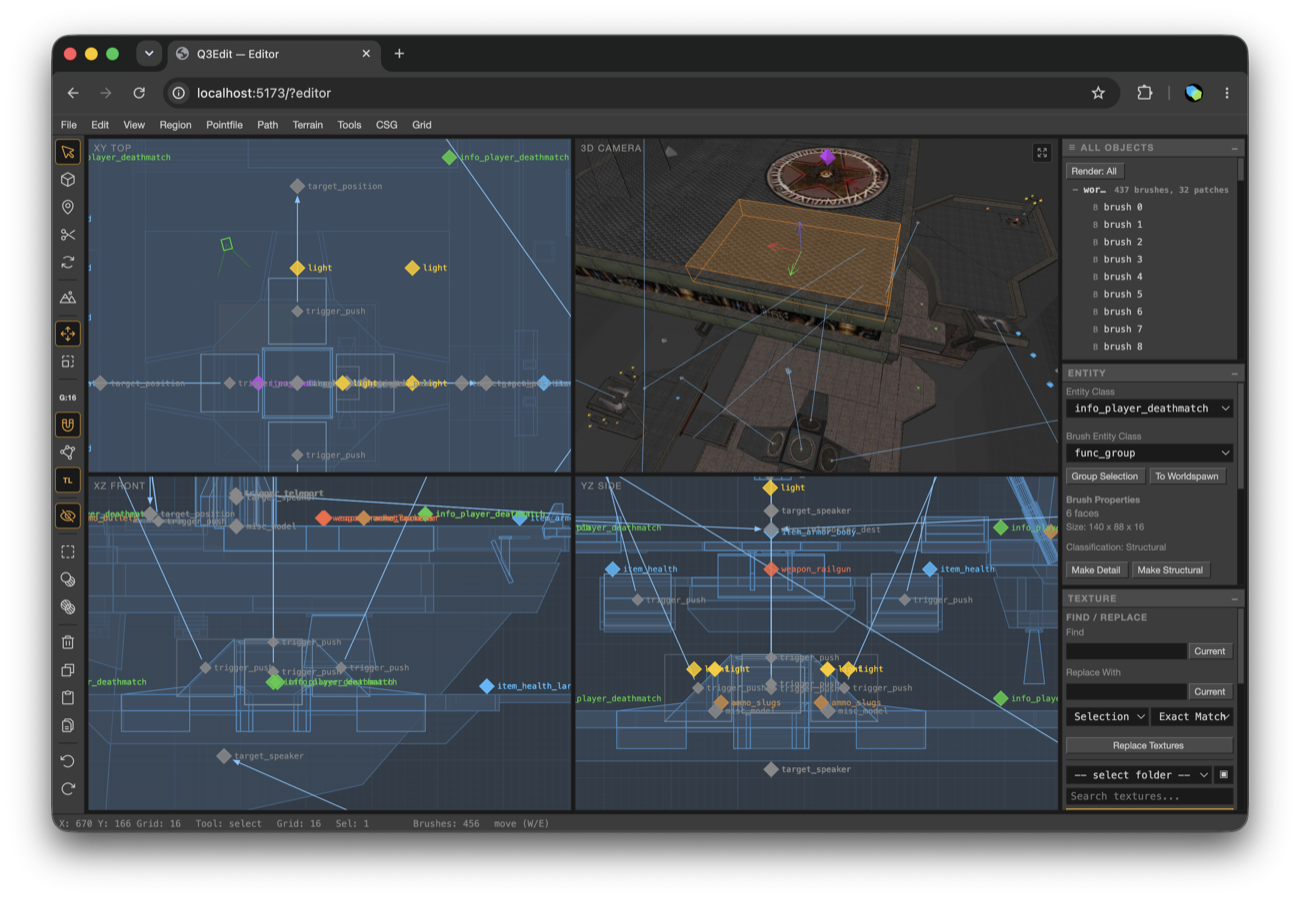
Real screenshot — the editor running in a browser tab
Stenchill: 3D Printable Solder Paste Stencil Generator
Your PCB stencil, 3D printed
Upload your Gerber files, get a 3D-printable file in seconds.
rocket_launchHow it works
1
Upload
Your Gerber ZIP file (KiCad, Eagle, Altium export...)
2
Preview
View the stencil in 3D and adjust settings if needed
3
Download the STL file and print it on your 3D printer
play_circleBarbatronic uses Stenchill
Barbatronic is a French maker and robotics creator. On Twitch since 2019, he publishes hardware tutorials on YouTube, runs an active Discord community, and is a member of the Karibous team, which competes every year at the French Robotics Cup. A community of curious hackers and hands-on makers shows up each week for his practical hardware insights.
Stenchill was actually born in one of his streams. A chat discussion convinced me the idea was worth building and that I had the skills to ship it.
In this video, he integrates Stenchill into his fabrication workflow and shares his first impressions.
help_outlineWhat is a stencil?
A stencil is a thin plate with openings matching the solder pads on your PCB. Place it on the board, spread solder paste with a squeegee, then position your SMD components before reflow. The result: precise and uniform paste deposits, much faster than using a syringe.
precision_manufacturingDesigned for prototyping and small batches
3D-printed stencils work best with 0603+ passive components and large-pitch ICs. For finer components (0402, fine-pitch BGA), a laser-cut stencil is recommended. Use a 0.2mm nozzle for best results on small pads.
starWhy Stenchill?
- A professional stencil costs $15-30 per side, here it's free
- Generate your file in seconds, print it the same day
- Print it at home on your 3D printer
- Perfect for old PCBs: get a stencil after the fact, no need to reorder
- Built-in registration shoulders for perfect alignment
menu_bookComplete Guide
New to 3D-printed stencils? Read our step-by-step guide to get started.
extensionKiCad Plugin
Use KiCad? The plugin complements the website by letting you launch a generation directly from the PCB Editor. For 3D preview, it's right here!
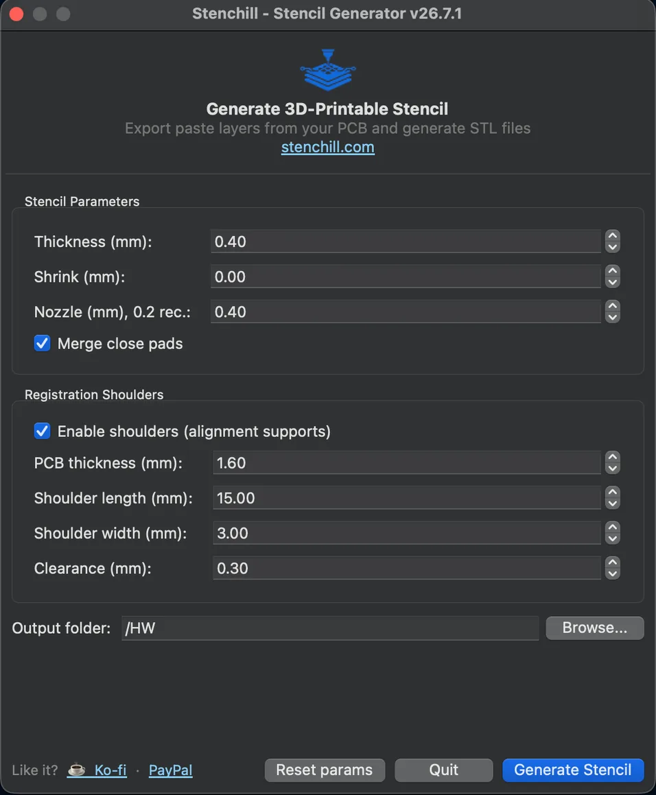
lightbulb3D printing tips
Material
PLA or PETG
PLA works great, PETG offers slightly more rigidity
Print bed
Smooth surface
Glass, smooth PEI or mirror gives a flat face that spreads paste cleanly
Nozzle
0.2 mm
Recommended for best results. A 0.4 mm nozzle is still acceptable
Layer height
0.1 mm
Essential for a smooth surface and good paste application
Stencil thickness
0.3 - 0.4 mm
3 to 4 layers at 0.1 mm. Thinner = less paste, thicker = more deposit
Infill
100%
Full infill ensures stencil rigidity
Wall generator
Arachne
Variable-width walls for narrow pad openings
Print speed
30 - 40 mm/s
Slow speeds give cleaner pad edges and avoid skipped fine features
photo_libraryGallery
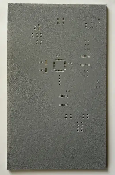
3D printed stencil
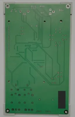
Stencil with registration shoulders

Solder paste application
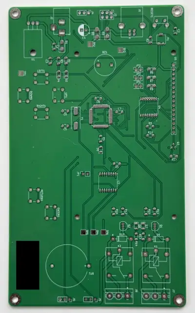
Paste deposited on PCB
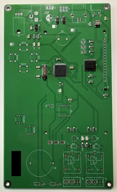
Components soldered after reflow
I started a “dirt notebook”
I love taking notes, but one problem that I have is that that I start cherishing every notebook that I start. I can't seem to keep my notes messy. Eventually, I start structuring the notes, doing cleaner handwriting, adding a cover or some stickers ... and before I know it, the notebook is too well-organised for simply scribbling into. This, of course, raises the hurdle for taking more notes and makes me start a new notebook, where the same process repeats again. It's a vicious circle. It won't surprise you that I'm somewhat enamored with the concept of shitty / messy notebooks, like this or this.


In an attempt to change this, I've started a dedicated "dirt notebook" now. I've nicknamed it "The Drainage Channel", because it's just a place for whatever is going through my head right in that moment. I'm using an old, empty notebook that I found lying around the other day. The paper quality is pretty bad; every kind of fountain pen ink bleeds through so I'm forced to use cheap ballpoints and it doesn't open flat, which makes it hard to take clean-looking notes in. I've been writing in it for about a week now, and it's been a lot of fun. I've used it to write down random quotes from podcasts that I've been listening to, ideas for stories, memos on my life and how I want to change it, new things that I learned or want to learn about more in the future ... with no elaborate structure, all just scribbled down next to each other. It's been interesting going back at the end of the week and re-discovering thoughts or things that I had almost forgotten about again.
My goal for now is filling this first "dirt notebook" and learning to embrace the messiness. Once I've gotten used to it, I could see myself switching to better paper and fountain pen ink again.
The Computer at the Bottom of a Canal
Somewhere at the bottom of the Forth and Clyde Canal, buried in the silt, there is a box of custom silicon that was right about almost everything.
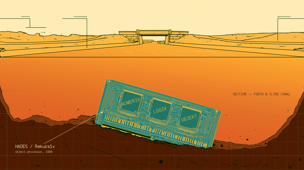
Somewhere at the bottom of the Forth and Clyde Canal, buried in the silt, there is a box of custom silicon that was right about almost everything.
Back in 1988 a Scottish hi-fi company shipped a processor that checked the type and bounds of every memory access in hardware, garbage-collected its own heap in silicon, and treated memory and disk as a single persistent object store. Retellings of the story make it out as charming folly, one where a company that made record turntables decided von Neumann was wrong.
But the story of the Rekursiv deserves to be more than just a curiosity, because almost forty years after it went into the water, its ideas are now shipping in production silicon from Arm; and also because the economics that killed it have just been reversed. Although all these years later, the fine details of the story mostly rest on the recollections of people who were there, it turns out that the hi-fi company were right about almost everything except which decade to build the hardware.
A hi-fi company builds a computer
Linn Products is the Glasgow company Ivor Tiefenbrun founded in 1972, and if you know it at all you know it for the Sondek LP12, still widely regarded by its partisans as the finest record deck ever made.
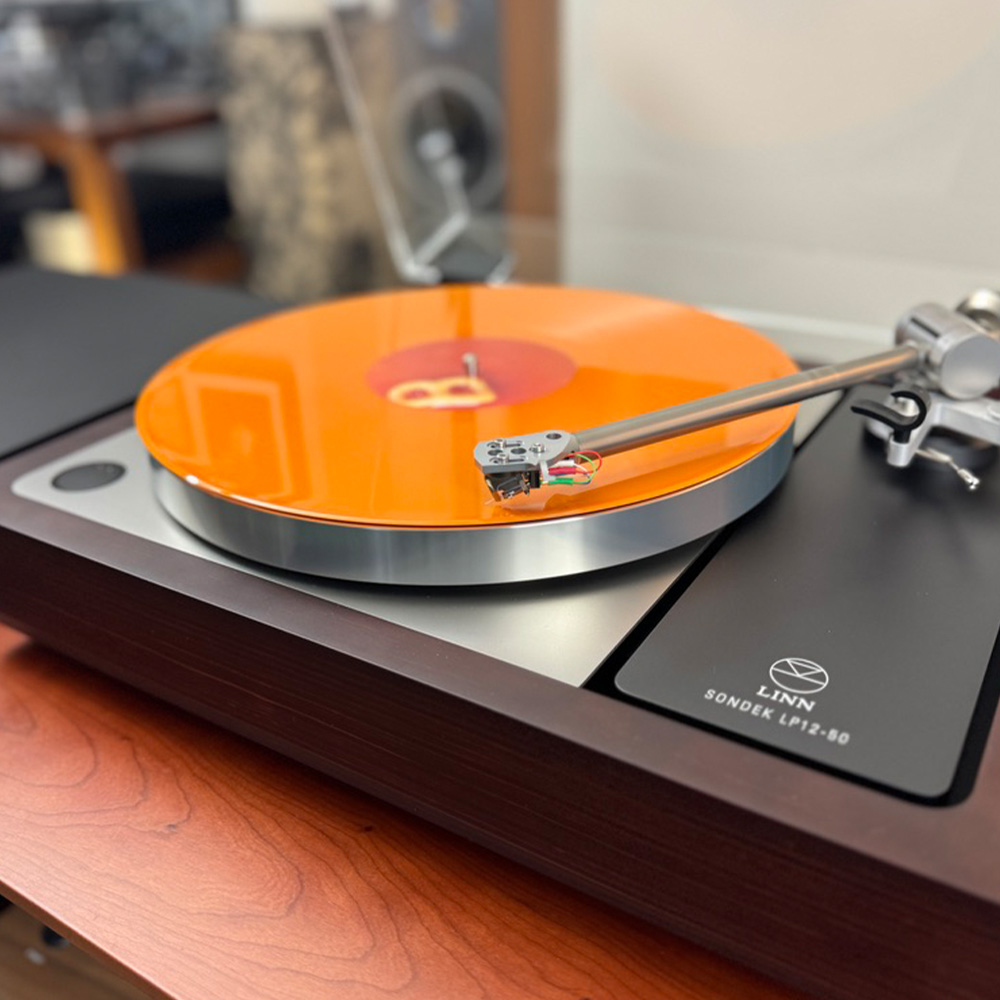
The Linn Sondek LP12
By the early eighties Linn had built a modern factory at Eaglesham, south of the city itself, and ran their business on a pair of VAX-11/750s along with a pair of 11/780s. But Tiefenbrun came to loathe the software they used. He wanted a system in which every physical object in the factory, down to each individual turntable moving through assembly, test, and even after-sales, had a shadowing software object accumulating its history (Pountain, Byte, November 1988).
So around 1981 Linn hired programmers and a University of Glasgow computer science lecturer, David Harland, and built an object-oriented language called LINGO. LINGO was a Smalltalk with some Algol in its syntax, not to be confused with the other Lingo programming language, which wouldn’t come along for another eight years.
MICRO$COPYTREE: entf 1 pagebus d=ustack
    crtf IDXBADTYPES newtrbr _CONS
    incmsp m.sp' newmptr
    jf MICRO$COPYTREE ldustk d=pgrorr     // the CDR branch
    m.fp 1 uaddbr newmptr
    readustk
    pagebus d=ustack
    idx2 newsr newbr loadaddr
    idxget nocheck incmsp m.sp' newmptr
    jf MICRO$COPYTREE ldustk d=memout     // the CAR branch
    js RTN$CONS
    rtf
Microcode for a recursive tree-copy instruction. Note the instruction calling itself, something forbidden to a conventional CPU (Source: Pountain, 1988).
LINGO worked; but it also ran far too slowly on the VAX to automate anything. Tiefenbrun’s response was pure Tiefenbrun. The hardware was the problem, not the software: so Linn would build hardware.
While stranded on a delayed train home from a seminar, Harland, and another computer engineer Bruno Beloff, sketched the repartitioning of their prototype into custom chips they christened “Rekursiv,” which is why Harland later joked that “the Rekursiv [was] British Rail’s fault.”
A few years later, in 1984, Tiefenbrun formed Linn Smart Computing, installed his brother Marcus as managing director and Harland as technical director, and funded it with Linn’s own money plus roughly £10 million from the Department of Trade and Industry.
LSI Logic fabricated the chips. Four gate arrays in 1.5 micron CMOS, 299 pins each, named NUMERIK, LOGIK, OBJEKT and KLOK. A company that sold the Sondek, the Ittok, and the Asak was never going to name the chips anything else.
Objects all the way down
What made the Rekursiv strange was not that it ran object-oriented programs. It was that a programmer – or, come to that, the compiler – could never see an address. Every object carried a 40-bit number issued at creation, and the OBJEKT chip translated numbers to physical locations through a hashed pager table, checking the type and the bounds of every single access in hardware as it went. Run off the end of an array? The machine refused. Forge a reference? The machine refused. Since only OBJEKT ever knew where anything physically lived, objects could be relocated freely without touching a reference, so garbage collection went into the silicon too: a two-space compacting collector that walked the live objects and slid them into the other half of DRAM while execution carried on above, oblivious.
Persistence worked the same way. Memory and disk were one object store, and if a needed object wasn’t in DRAM the processor simply stalled, mid-instruction, while an external disk processor fetched it, then carried on as if nothing had happened. Because paging sat below the level of instruction execution, a single microcoded instruction could be arbitrarily complex, and could even call itself. That’s the recursion in the name. There was no fixed instruction set at all; the instruction set was a loadable artefact, and you gave the machine whichever one suited your language. Linn supplied C, James Lothian microcoded a Prolog instruction set, a Manchester group put Scheme on it, and Aberdeen ported the persistent language PS-algol. I am a St Andrews alumnus who was around at the right (or if you want to look at it like that, the wrong) time. I can still remember more than I’d want to about PS-algol. But that, as they say, is altogether another story.
The numbers Linn claimed were spectacular. A CONS cell every two microseconds, twenty times the speed of Lisp on a Symbolics workstation, and Prolog unification as a single instruction. But the figures came from Linn’s own simulations, reported in Byte magazine with the company’s cooperation, and nobody ever reproduced them independently.
The attack of the killer micros
The Rekursiv belonged to a respectable intellectual tradition. Through the seventies the industry consensus held that hardware should rise to meet the language, closing what the literature called the semantic gap; Intel bet its first 32-bit design, the object-oriented iAPX 432, on exactly this, and Symbolics built a workstation business on Lisp in microcode.
Unfortunately for the Rekursiv that tradition was demolished in public at almost the exact moment Linn committed to it. Patterson and Ditzel made the case for RISC in 1980: compilers use a fraction of a complex instruction set, the complexity taxes the common case, and simple instructions plus caches plus good compilers go faster. By 1984 Berkeley’s SOAR project had run Smalltalk, the canonical dynamic object language, fast on a simple chip of thirty-five thousand transistors. The Rekursiv’s central assumption was publicly undercut four years before the first board powered on.
Then the economics arrived. Commodity microprocessors improved at roughly 52% a year from 1986 to 2003, the period Eugene Brooks of Lawrence Livermore christened the attack of the killer micros. The Rekursiv took four years to design. It was conceived when a VAX defined respectable performance, and in 1988 it emerged into a world of SPARCstations and 386s, with the 486 arriving close behind.
Lothian, who was there, put it plainly enough five years later: the machine simply couldn’t hold its own against the new workstations. Around twenty or thirty boards were built. Most went to universities. There’s no record that suggests one of them ever ran Linn’s production line, which was the entire point of the exercise. The one field comparison that survives has a threaded-code LINGO on a Sun-3 running about twice as fast as the Rekursiv board it was meant to be inferior to, and which was designed with the intent of running it.
The end was memorably Glaswegian. Black Monday had squeezed Linn’s finances, a venture rescue never closed, and the final straw was a car park. A Linn delivery driver reversed a van into Harland’s Porsche, Tiefenbrun declined to pay for the repair on the grounds that it happened on private ground, and Harland resigned.
On his way out he threw his own accumulated hardware and backup media into the Forth and Clyde Canal. The version of the story where the whole product line goes into the water is better; but the truth is good enough.
At least one complete board escaped, and sits today in the Jim Austin Computer Collection near York.
Linn, meanwhile, recycled the name Numerik for the DAC in its CD range, which is as good a headstone as any. Harland left computing entirely around 1995 and became one of the most prolific historians of spaceflight, several dozen books and counting. As a recovering astronomer myself, I can only approve of the career change.
Right about everything?
But here is why this is all more than an historic anecdote. Because I think we need to take a hard look at the Rekursiv’s four defining design decisions, and then ask where each one stands today.
Hardware memory safety
OBJEKT checked the type and bounds of every access against references the program couldn’t forge. That’s a working description of CHERI, the capability architecture Robert Watson and colleagues have been building at Cambridge and SRI since 2010, in which every pointer carries hardware-enforced bounds, permissions and an unforgeable validity tag.
Arm built it into the Morello prototype boards it shipped in 2022 under the UK’s Digital Security by Design programme, and ships the lighter-weight Memory Tagging Extension in Android phones today.
Microsoft’s security team concluded in 2020 that CHERI would have deterministically mitigated at least two thirds of the memory-safety vulnerabilities it patched in 2019. The idea that the object, with its type and its bounds, is the proper unit of hardware protection has gone from eccentric to frontier.
Garbage collection as an architectural concern
Azul Systems spent the 2000s selling Vega appliances, custom multicore processors with hardware read-barrier support, to make pause-free collection practical for Java heaps; the C4 collector that came out of that work now runs in pure software on commodity x86. The algorithm survived the move; the custom silicon stayed behind.
The single-level persistent store
IBM shipped single-level persistent stores in the System/38 in 1978, carried it through the AS/400, and it survives today as IBM i; Intel spent billions trying to reboot the idea as Optane before winding it down in 2022, and the same ambitions are now migrating into CXL memory fabrics. An idea the market keeps finding reasons to want, and reasons not to pay for, is different from a bad idea.
Silicon shaped to a workload rather than to everything
This is the biggest design decision: the one that is now just the way the industry works. Hennessy and Patterson, the two people most responsible for burying machines like the Rekursiv, spent their Turing Lecture arguing that domain-specific architectures are the only road forward now that Dennard scaling is dead and Moore’s Law is wheezing. Or to be more honest, also dead.
Google’s TPU, Groq’s deterministic streaming processor, Cerebras’s wafer-scale engine and Etched’s transformer ASIC are all machines built to run one computational language well; it just happens that the language is now linear algebra rather than Smalltalk.
Four for four
Every architectural conviction that went into the canal with the Rekursiv is either shipping, in production, at scale, or is the declared direction of an entire field. Four correct calls in a row is too many for luck. The likelier reading is that the almost forty years in between were not the natural state of computing but an accommodation to a scarcity, and that the scarcity has since gone away.
I made a different version of this same argument back in June, about software rather than silicon. In my essay a distribution of one I argued that bespoke software was the original, correct arrangement, that fifty years of productised general-purpose software were a compromise forced by the economics of scarce programmers, and that AI has ended the compromise.
The general-purpose commodity processor was also a compromise, forced by a 52%-a-year improvement curve that made any bespoke architecture obsolete before it reached silicon. That curve is gone. The compromise is going with it; and the workload-shaped machine, the thing Harland was building in 1984, is what comes back.
Where the semantics live
The comfortable lesson, and the one usually made about the Rekursiv, is that you don’t fight the commodity curve. This is true, but no longer very useful, because the curve is dead. The useful lesson is subtler, and you can see it when you think about why IBM succeeded with the same ideas at the same time.
The System/38 had the Rekursiv’s deepest commitments: single-level store, persistent objects addressed by name rather than address, capabilities, everything an object. It thrived for decades because IBM put those semantics in a virtual instruction set, the Technology Independent Machine Interface (TIMI), and translated to whatever processor was underneath. When the platform moved to PowerPC in 1995, customer applications didn’t even need recompiling. Linn welded the same semantics into four specific gate arrays. The abstraction is still running today; the gate arrays lasted five years.
Interestingly enough, Britain has run this experiment more than once, but with very different outcomes.
Acorn, another small British company with contrarian silicon convictions, designed the ARM 1 in 1985; and the business that conquered the world was not Acorn’s computers but the licensing company that sold the abstraction, an instruction set anyone could implement on whatever process node the commodity curve offered next.
Inmos, meanwhile, welded David May’s genuinely brilliant parallel architecture into the Transputer, was outrun by exactly the same curve that took the Rekursiv, and survives today mainly as lineage: May’s XMOS, and Bristol’s continuing habit of contrarian silicon, through to Graphcore. Put the ideas above the silicon and they can outlive any particular chip. Put them in the silicon and they live exactly as long as the process node does.
Everyone needs a canal
The Rekursiv was hardware reshaped to fit a language, because the general-purpose machine fitted the language badly. What’s happening now is the same move in reverse: a whole class of new languages reshaped to fit a machine, because general-purpose languages fit LLMs so poorly. There are enough of them now to fill a catalogue, which I maintain at agentlanguages.dev, where they split into camps that disagree about almost everything except the diagnosis.
Vera, the language I released back in February, is mine. But the instinct underneath all of them is the one Harland was acting on in 1984: that the substrate should change to meet its authors. For him the authors were human and the substrate silicon. This time the authors are models and the substrate the language. Harland made his bet at the worst possible moment in the history of the commodity curve. I’d like to think mine is better timed. The canal is patient either way.
The second time around
Which brings us to why I’m writing about a dead Glaswegian computer.
Our thesis at Negroni has always been that technology waves are cyclical, and that reading the cycle matters more than reading the technology. The Rekursiv is the cleanest case study I know of a team that read the technology almost perfectly and the cycle catastrophically: right about memory safety, right about garbage collection, right about persistence, right about workload-shaped silicon, and wrong about what year it was needed.
The team at Linn were insanely early with a design philosophy which was, to put it politely, exotic at the time. It’s only now, all these years later, that we know they were right.
Judged on its ideas, the Rekursiv holds up embarrassingly well. It’s only judging the execution which makes every decision look wrong. But being right too early is not a business model.
The reason to tell the story now is that the cycle has actually turned. The 52% curve that killed every bespoke architecture of the eighties ended twenty years ago; RISC-V and modern tooling have collapsed the cost of taping out something opinionated; and the government money is even flowing again: DTI millions into Glasgow back then, Digital Security by Design millions into Cambridge and Morello today.
For the first time since Harland stood on that canal bank with a cardboard box full of silicon, a small team with a contrarian conviction about what silicon should do is not automatically doomed by the calendar. That’s precisely why Negroni looks at silicon companies, and when we do, the Rekursiv is the checklist I follow. Is the workload broad enough to pay for the transistors? Do the ideas live above the silicon or welded into it, and does the team know what the compilers will do to them?
Somewhere at the bottom of the Forth and Clyde Canal there’s a computer that was right about almost everything. The ideas behind it took almost forty years to make it back to the river bank, but every one of them has made it to shore. This time around, our job needs to be keeping the silicon out of the water.
Lego building instructions through time
The silent helper that without a single word guides you, step by step, to transform your pile of bricks to fantastic creations.
Building instructions. The silent helper that without a single word guides you, step by step, to transform your pile of bricks to fantastic creations. The tool that shows you building techniques and gives you a solid foundation for further exploring the wonders of the LEGO® brick. Let’s take a look at some of the many historic milestones.
Before instructions
The history of building instructions starts with very simplified instructions as early as 1955. Prior to this the only ‘guidance’ for products containing plastic bricks were drawings on the packaging to serve as inspiration for consumers. There were also examples of small leaflets with inspirational material inside some boxes in the 1950s.
box of automatic binding bricks
Example of a set with drawings on the packaging
The company also produced more elaborate inspirational material to hand out or sell separately, the so called “byggebog”, which directly translates to ‘building book’, but perhaps a better term is idea book. The Idea book was first published in 1955 and contained among other things information on different building techniques and inspiration for building houses.
Cover of LEGO® Idea book from 1955

Spread from the book concerning building techniques
Early building instructions
In 1955, the LEGO® System in Play idea was introduced. The groundbreaking idea that among other things makes sure the bricks you buy today will fit with the bricks you bought yesterday and the bricks you buy tomorrow. The first LEGO System in Play products were centered around a town environment (Town Plan no. 1). The town plan and the houses and shops etc. to inhabit the town was the first time the LEGO Group introduced special sets with specific models, as in, the model you saw on the box was also what you could build with the content of the box. This created a need for more instruction to make sure all consumers could reach the wanted result and thus the first simple building instructions were introduced. Although instructions for specific models started to appear there was also a focus on encouraging alternate builds as the below instructions also shows. In the text to the left, it was suggested to build the two buildings together with other buildings on the town plan to create “nice corner shops”.
Example of a simple instruction for a 1955 set intended for the Town Plan
Sketches for some of these instructions found in the LEGO® Group Archives suggest that these early pioneering instructions for LEGO sets were most likely made in-house
Just as the new specialized Town Plan sets with building instructions had a hint of free building/alternate builds in them, the basic sets, with a high degree of free building, started having suggestions for instructions. From 1955 onwards, simple instructions for houses were found in basic sets to serve as inspiration/play starters for consumers. This mirrors the different views present in the company at the time. For example, documents reveal an internal discussion in 1960 where the company’s management have different views on how much “help” consumers should receive when building with LEGO® bricks. Should you only provide inspirational material and let children’s imagination do the rest or do you “educate” children with instructions and thus building techniques in the hope that by doing so you instill confidence in children to investigate the endless building possibilities of the LEGO system later in their play journey. The material available in the early 1960s suggests a compromise and the above-mentioned observation hints at a similar situation in the mid-1950s.
Building instructions for suggestions for houses you could build with various basic sets such as set no. 700/1, 700/2 etc.
More elaborate instructions
From the introduction of the LEGO® brick, we know today, in 1958 and the much-improved stability that came with the ingenious interlocking principle, LEGO sets slowly became bigger and more detailed and this demanded a change in building instructions in the early 1960s. From then the instructions slowly started to contain more building steps than earlier, and the building experience was improved by consistently adding color to the instructions. However, the instructions were still very simplified compared to the ones we have today. The instructions would normally have two sides with one showing steps to build the model depicted on the front of the box and the other side would contain images of alternate builds. Going back to the beforementioned internal discussions it seems we are still looking at the art of compromise.

Building instruction from 1964, set no. 323, showing instructions on one side and alternate builds on the other
Although the material is scarce on the subject, the change in building instructions indicate approximately when the LEGO Group started to team up with external companies to help us draw the instructions.
We know for a fact that from 1967 and until 2003 the main supplier of drawing building steps for the LEGO Group was a company called Palle Munch, Grafisk tegnestue & Reklamebureau based in the Danish town Kolding. However, according to the owner Palle Munch, some instructions were made by another company in Aarhus, Denmark.
Creating Building Instructions
Speaking of drawing building instructions, let’s look at some of the many steps it took to create a building instruction back in the day. Making building instructions was a slow and tedious process. After the designers finished designing and building the model it would be split down into the various building steps – for many years the building steps were decided by the designers themselves. Every building step would be built and put next to each other on a table for review and approval. After being approved pictures would be taken of all the steps, one by one. Each model showing one building step was meticulously placed exactly on the same spot as the previous one and then the next step would follow. Eventually you would be able to match the pictures over each other to form a section by section building instruction. The photos were sent to external partners, like Palle Munch, Grafisk tegnestue & Reklamebureau, who then drew the building steps by hand. The drawings were made in a larger scale (each knob had a diameter of 7,5 mm) to make the detailing easier. Afterwards the drawings of the building steps were scaled down and sent to another company for the finishing touch - coloring. Palle Munch also remembers the physical building steps being shipped to him in boxes, sometimes taking up a lot of room on the company’s premises. This would happen later when Palle and his employees started using other technologies to draw the building steps…
A big change
In the early 1980s, big changes were happening in the world of LEGO® building instructions. In 1983, the LEGO group sets up a specialized building instruction team for the first time who take over creating the building steps from the designers. A few years later a switch is made from hand drawn building steps to doing it in a computer-based tool instead. Palle Munch, the owner of Palle Munch, Grafisk tegnestue & Reklamebureau finds a 3D drawing tool called ‘Monster’ which originally is used to draw stage settings for Danish television. In May 1984, Palle Munch contacted the company who originally created Monster and asked them to help create a new tool suitable for drawing building instructions for LEGO sets. The project started in the fall of 1984 and the intention was to use Monster as the basis to create the new drawing tool. Quickly the company behind the original tool realized that the task of making a tool for drawing building steps required a quite substantial rebuild of Monster and it took more than a year and a half to create the new tool. The tool, eventually called ‘Panter’, was named after Palle Munch, and the name stands for “PAlles Nye TEgneRedskab” which translates to “Palle’s new drawing tool”.
building instruction from 1988
Set no. 6675 from 1988 is an example of a building instruction created with Panter
Panter was used for creating LEGO building instructions for the first time in 1986 and remained in use for the next 17 years. Although Palle Munch and his team drew the various building steps with Panter and later Panter 2, an updated tool that now included colour, it was the building instruction team in the LEGO Group that had the last say. When a new building instruction was being made, Palle Munch and team would send a test instruction to the LEGO Group for review. After review, the building instruction was changed according to the comments made by the building instruction team before the final instruction was created.
image of test building instruction
Example of a test instruction from 1998 made on Panter 2 with handwritten corrections from the building instruction team at the LEGO Group
New tools
In 2003, a new tool ‘3D Vision’ was introduced and replaced Panter. 3D Vision was considered a large step forward. The new tool was much more user friendly than Panter. With Panter a lot of data had to be added in the system manually for each individual LEGO® element, but in 3D Vision this information, such as, dimensions etc. was automatically generated in the system. This made the new tool much more time efficient. In an article in an internal employee magazine in 2003, concerning the introduction of 3D Vision, it was mentioned that the new tool created a building instruction for a new LEGO Technic set in 3 days, and an employee was quoted for saying that with Panter it would have taken 3 weeks. Also, in 2003, 36 years of collaboration with Palle Munch, Grafisk tegnestue & Reklamebureau ended as the LEGO Group wanted to bring the whole process of making building instructions in house.
image from building instruction from 2005
Page from a building instruction made with 3D Vision. Set no. 7239, from 2005
Approximately two years after the rollout of 3D Vision a new tool was introduced. The development of Easy Builder Tool (EBT) started in 2004 and in 2005 it was used to create the first building instructions. Contrary to 3D Vision, EBT was an internally developed tool. The tool was a plugin for an already existing externally developed 3D platform. Compared to 3D Vision the new tool came with more elaborate features but it was also known as a more complex tool to master.
page of building instruction from 2006
Building instruction from 2006 created with Easy Builder Tool
Expansion
In recent years the building instruction team has grown a lot due to, for example, a growing product portfolio. Starting with 2-3 people in 1983, the building instruction team now consists of more than 100 employees across various teams and functions. They use several tools to create the fantastic building instructions you find in LEGO® sets today. One of the main tools being LEGO Digital Designer (LDD) Pro. The first instructions made with LDD Pro go back to 2018 and from 2022 all LEGO building instructions have been made exclusively with the tool. How are current building instructions made you ask? Well… that is a business secret!
Which is which?
Throughout this article, examples have been shown of building instructions made with the different tools we have had over the years. If you are struggling to see a difference in the different instructions from different time periods you are not alone. The “cartoonish” look of the instructions is something, with a few exceptions, we have always aimed for. The simple reason being that it works, and you can easily distinguish various colors and shades from each other. A LEGO® building instruction is not about portraying the model as lifelike as possible, it is about creating the best possible building experience.
LEGO® Builder
Since the 1950s LEGO® building instructions have been a paper-based friend in need for consumers wanting help to tackle the vast possibilities of the LEGO system in Play. Today, building instructions are more than ‘just’ paper instructions. They can also be experienced through the LEGO Builder app giving consumers, no matter their experience level, an easy and intuitive building experience. In the app you will find instructions in both 2D and 3D. The latter allows you to zoom and rotate to view your build from all sides. One of the most intriguing features is unlocked when you press the ‘build together’ button on select sets in the app. This allows consumers to build a LEGO set as a team by delegating each builder a building task to complete. There is a place for everyone, no matter what skill level you have, and the feature is a fantastic tool for family quality time or teambuilding.
Relentless pursuit
LEGO® building instructions have come a long way from the simple instructions in 1955 to LEGO Builder, but to this day one thing has never changed… The relentless pursuit from dedicated employees towards worldclass intuitive building instructions aimed at creating a solid foundation for LEGO builders to further explore the LEGO system in Play.
Tech note: making your own V-I plots at home
My beef with the diagrams in popular electronics textbooks and online tutorials is that most of them are fake.
Or, how to lose money with friends.
When working on my latest book, The Secret Life of Circuits, I wanted to keep the artwork real. My beef with the diagrams in popular electronics textbooks and online tutorials is that most of them are fake. At best, they’re retraced from ancient texts; at worst, they’re sketched from memory and can be charitably described as “inspired by true events”:
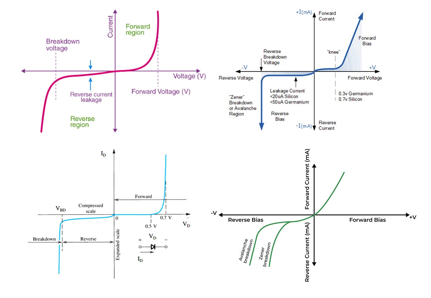
An assortment of V-I plots for diodes, collected on the internet.
The Secret Life of Circuits contains about 290 original illustrations and does its best to avoid such shenanigans. I painstakingly gathered real data for everything from quartz crystal frequency response, to battery discharge curves, to signal reflections in a 100 ft run of coax cable strewn around the workshop, to the behavior of vacuum tubes.
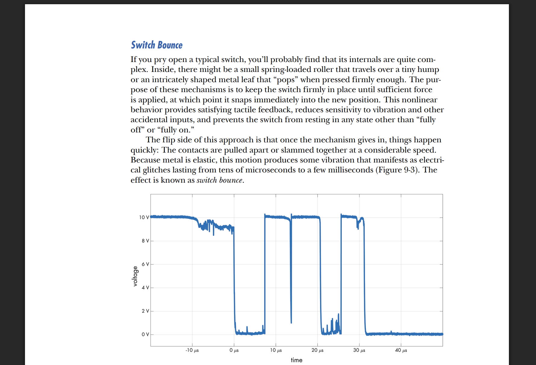
A snippet from the sample chapter, available here.
Most of it was straightforward to capture, but I can’t say the same about the parametric plots that show the relation between voltage and current in semiconductor devices. In some portions of the curve, the currents are too miniscule to record with the most common graphing instrument, the oscilloscope. In other portions, the current suddenly skyrockets — and before you know it, the device lets out the magic smoke. Even in the in-between region, there’s no respite: the characteristics of semiconductor junctions change with temperature, and that includes self-heating due to currents as low as 1 mA. Do nothing and watch a point on the oscilloscope screen drift away.
To tackle this problem, I ditched the oscilloscope in favor of a benchtop multimeter (DMM) and pulsed power from a lab supply. The perk of the multimeter is that it can easily measure down to microamps and microvolts; the perk of pulsed power is that heating-indued drift can be kept in check.
Oh — I would also submerge the device under test in non-conductive liquid for cooling purposes. Mineral oil is a sensible choice, but many other options should do:
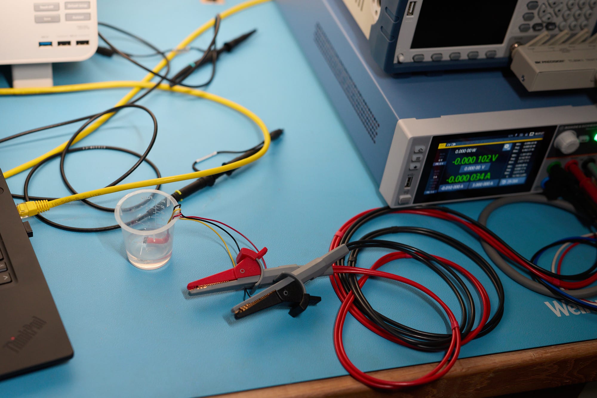
A close-up of the final setup.
Although I prepared some diagrams by manually writing down currents and voltages, this is obviously tedious and error-prone, so it’s better if one or more of the instruments can be interfaced to a computer. Many benchtop instruments support a simple, text-based protocol called Standard Commands for Programmable Instruments (SCPI). Depending on the age of your gear, the interface may be available over RS-232, via a USB Type B (printer-style) port on the rear, or via Ethernet — in which case, you simply establish a TCP connection to port 5025.
The SCPI protocol uses commands and queries. An example of a query is *IDN? followed by a newline (\n); sending this string causes the device to respond with a line of text describing its make, model, and other identifying information. Another possible query is MEAS:VOLT?, which might return the current voltage reading. In contrast to queries, commands do not return any text; an example may be SOUR:VOLT 1.2 to set the voltage to 1.2 V, or OUTP 1 to turn on output channel 1.
Alas, although I had an SCPI-capable multimeter, my benchtop power supply was more basic and offered no remote control; without it, the process was still half-manual. Fed up, I eventually purchased a source measure unit (SMU) — essentially a combination power supply and a multimeter with a very fast response time. Brand new SMUs are obscenely expensive, but there are virtually no second-hand buyers for them, so it’s easy to find excellent deals on eBay if you haggle a bit. I scored an unmolested Rohde & Schwarz NGU401 unit for a laughably tiny fraction of its astronomical MSRP ($9,000).
This particular SMU can be used by repeatedly setting the output voltage and then querying the DMM for the current on-screen reading, but the reading is updated only at a frequency of about 3 Hz. A better option is to use the device’s data streaming mode; in the Rohde & Schwarz parlance, this is known as FastLog. The API allows sampling rates of 100 to 500k per second (!) and sends voltage-current pairs as binary 4-byte floats.
Of course, as can be expected of a niche feature on a niche device, nothing actually works as documented. The most grievous problem is that the returned binary data is corrupted if you try to use the serial-over-USB interface; after a day of chasing ghosts, I was finally able to get it to work over Ethernet.
My C implementation for capturing the V-I curve of a forward-biased diode can be found here. It uses FastLog at 10 ksps; for currents below 0.3 mA or so, it leaves the supply voltage on and averages 2,500 data points to obtain a noise-free microamp-range reading. For higher currents, it cycles the power on for 5 ms, and averages the best 20 samples from the FastLog buffer.
The following plot shows the actual, positive-side V-I curve for a popular, small 1N4148 diode with a continuous current rating of 300 mA:
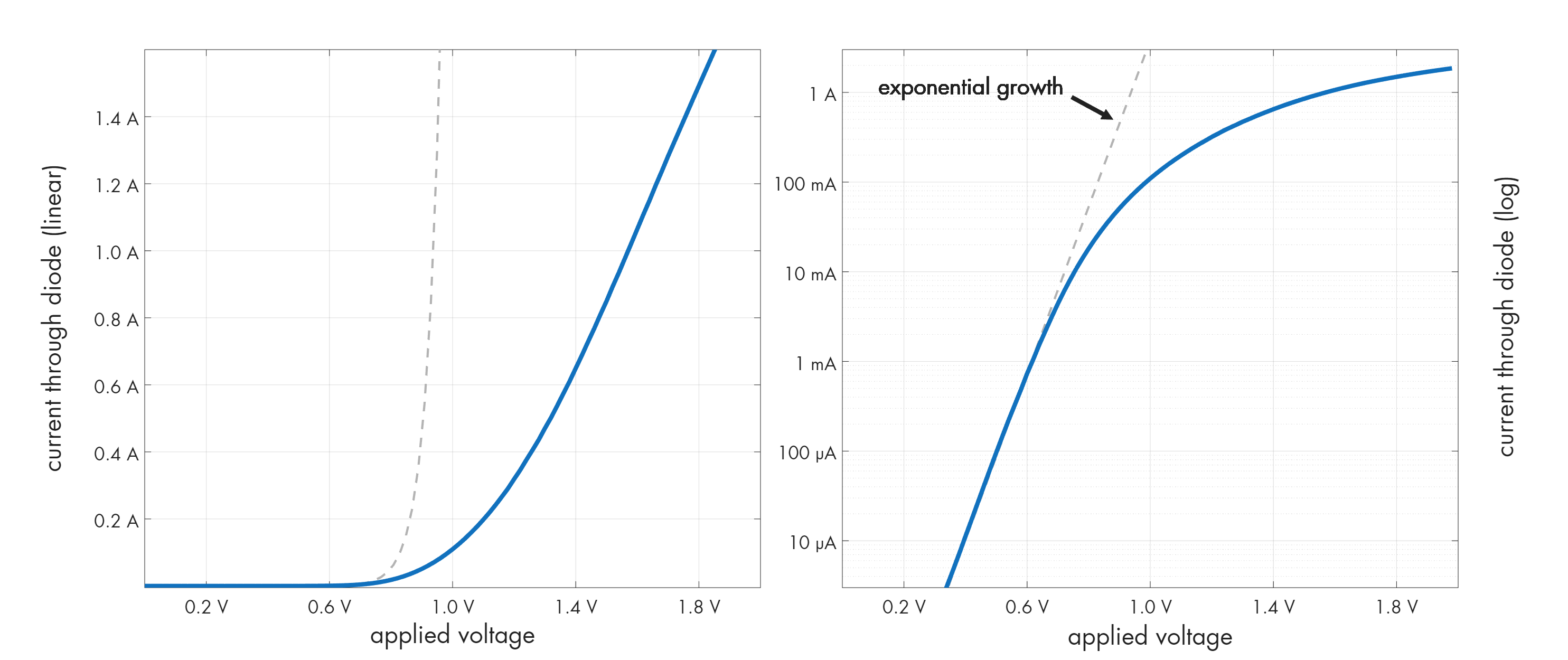
Forward bias of 1N4148.
Unedited measurement data can be found here. I was able to effortlessly cover the range from few microamps to nearly 2 A; it’s actually possible to go to 4 A, but it adds no interesting detail to the plot.
Note that although the relation between the applied voltage and current in a diode is often described as exponential, this is true only for modest currents. In the log-current plot on the right, we see that the property no longer holds in the vicinity of 10 mA; the curve diverges from the dashed line that represents an idealized model fitted to the initial, truly exponential slope. That’s because of resistive effects in the semiconductor substrate — and it’s one of many reasons why it pays to have real plots.
Diodes eventually begin to conduct when reverse-biased too, but in the case of 1N4148, the threshold is about -145 V, so it’s hard to capture all of the component’s dynamics on a single well-proportioned plot. We can do it more easily for Zener diodes. For example, the following was captured for 1N4731, a low-voltage Zener rated for 4.3 V at 58 mA:
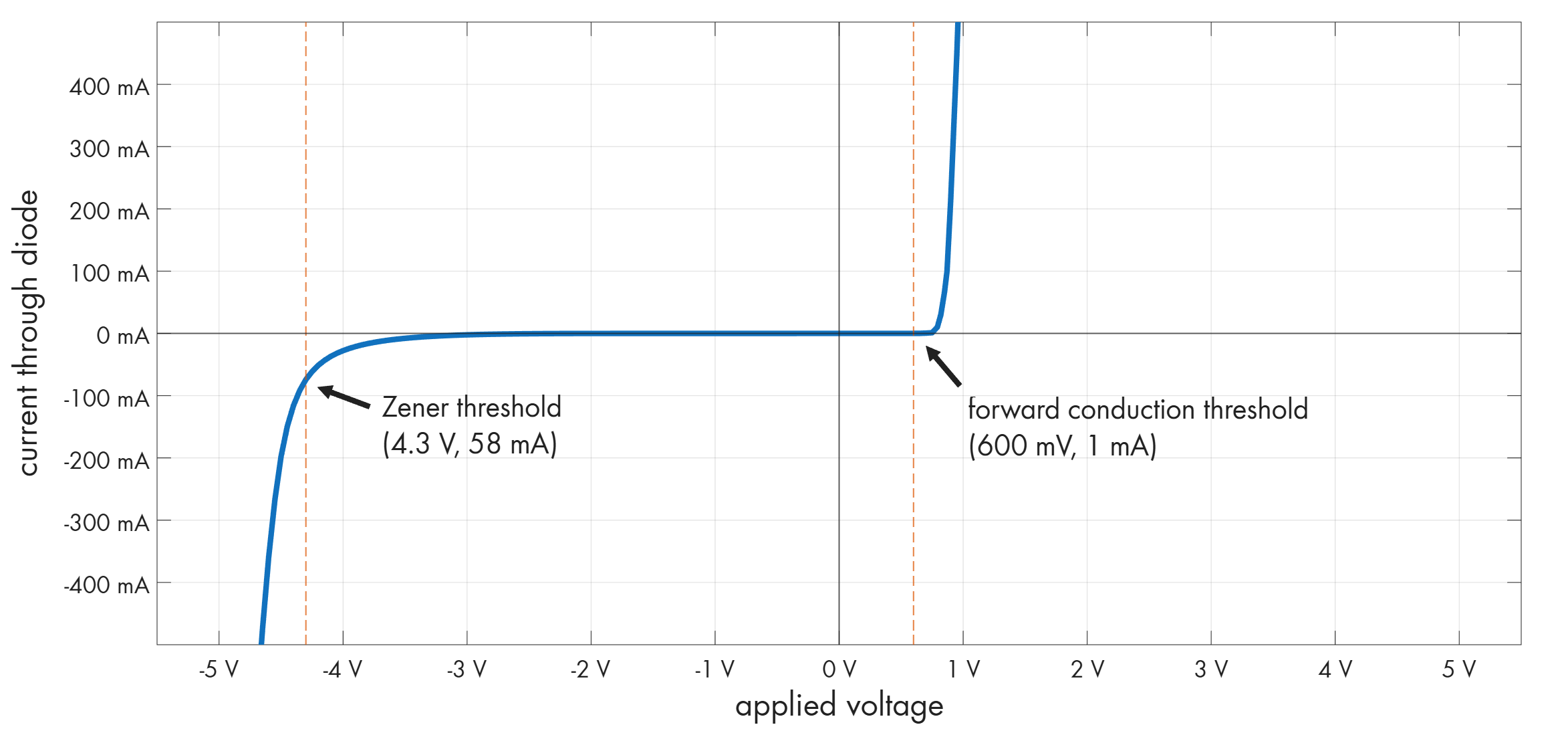
Real-world behavior of the 1N4731 diode.
In these Zener diodes, the reverse breakdown curve is not as steep as the response in forward bias; if you want to use the component to produce a specific reference voltage, you need to keep the current in the right ballpark too.
The same toolkit also works for transistors. For example, here’s my plot of the admitted current in relation to the drain-source voltage for a small MOSFET, BS170:
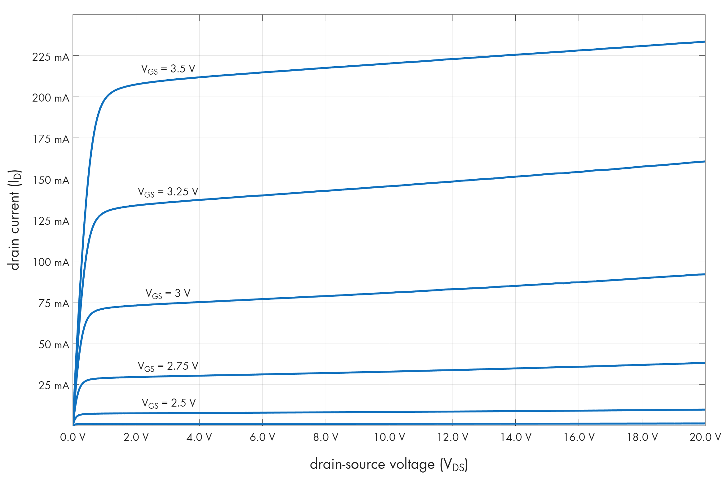
VDS-ID curves for BS170.
The plot shows that the transistor is more or less a constant-current device in the bulk of its usual operating range; the current limit is dialed in by the gate-source voltage (VGS) and changes less than 10% for VDS between 1 and 10 V.
We can also show what happens on the tail end of that curve. The spec for the transistor gives its breakdown voltage as 60 V; in textbooks, this is usually shown as a sharp transition to vertical. For example, variants of the following diagram have made it into countless online articles and scientific papers:
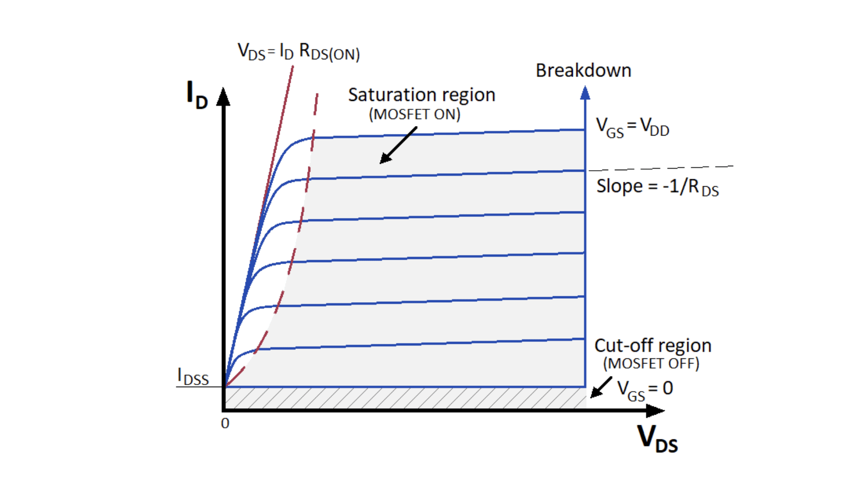
Yet, the reality is more nuanced:
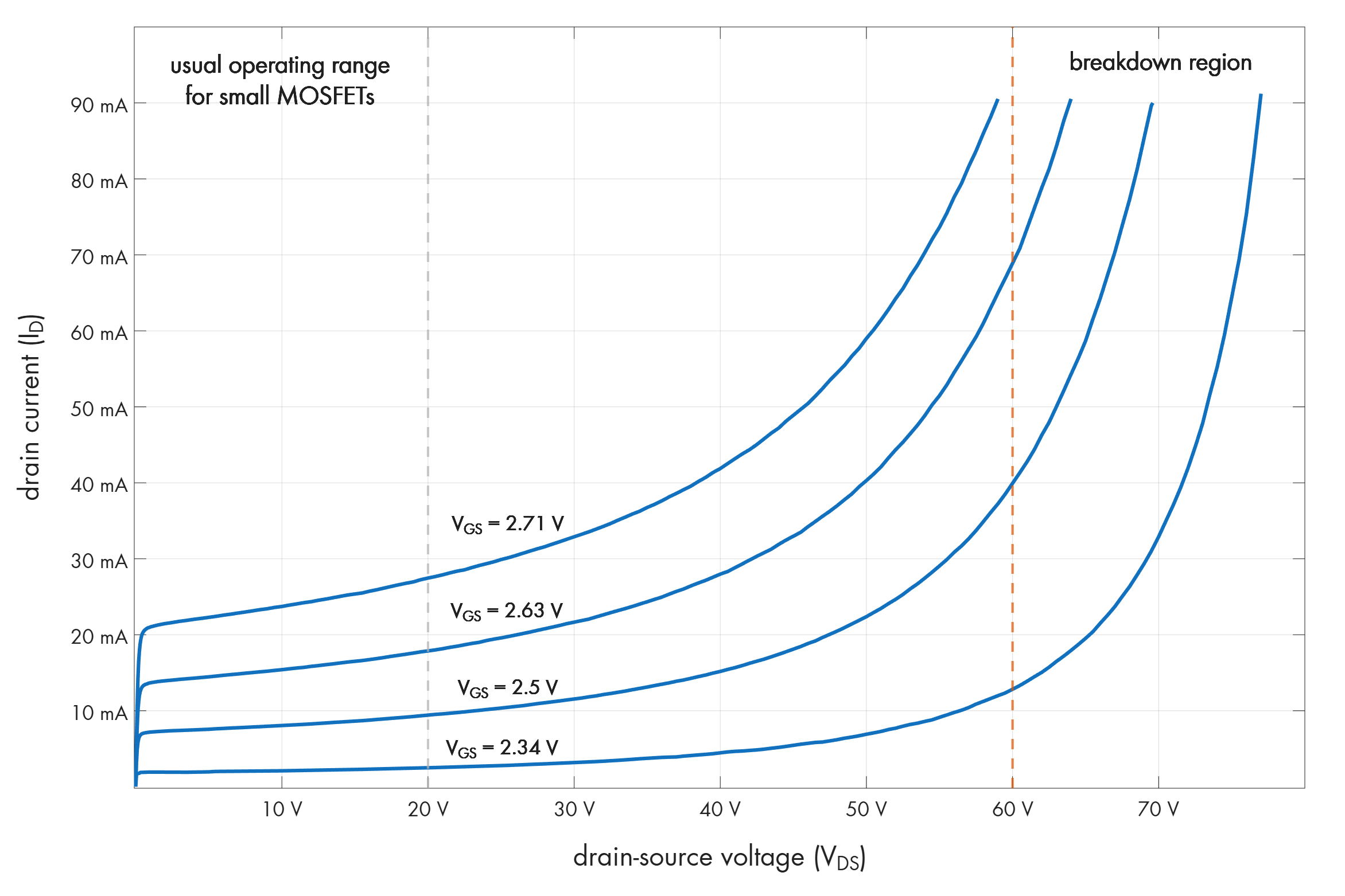
BS170 near the breakdown region.
In a nutshell, you get a relatively sharp and spec-compliant breakdown only at very low gate voltages; in fact, the behavior is diode-like for VGS = 0 V (not shown above). But if you’re supplying a more practically useful VGS, the build-up to the danger zone is more gradual and you’ll be in trouble well ahead of 60 V.
As a side note, that last plot required a bit of ingenuity: my source measure unit has a limit of 20 V. To gain extra range, I added a traditional, floating power supply in series with the SMU and then stitched the captures for several voltage spans. This solved one problem but created another: even with the SMU idling, there would be substantial drain-source voltage applied to the device under test, and for some values of VGS, it could be enough to heat up or even destroy the transistor.
To address the issue, I moved from a fixed VGS signal to 5 millisecond pulses delivered by a signal generator at a low duty cycle. I also modified the data logging code to sample the current continuously over the period of about 2.5 seconds, average the best results, and then move to the next voltage set point. Source code for this variant can be found here.
I'm Making Strandfall, a Solarpunk Orienteering Larp
Smartphones are anti-enchantment devices.
I’m Making Strandfall, a Solarpunk Orienteering Larp
In the twenty years I’ve been making games, I keep returning to the idea of blending the digital and physical worlds through ARGs like Perplex City and location-based games like Zombies, Run! It’s as if the act of mixing worlds enchants them both. That impulse is probably why I recently became fascinated by Nordic Larp (live action role playing), the closest thing we have to a fully embodied, truly participatory avant-garde art form today.
So for anyone who knows me, it’s probably no surprise that my next game, Strandfall, combines all those notes. Strandfall is a highly physical outdoor larp that I’m co-creating with Alex Macmillan as part of our new collective, Experimental Social Scene, supported by Immersive Arts funding.
This September, 30 players will embark on a desperate expedition in a real park in Edinburgh to uncover the nature of mysterious storms that are ravaging the world. Over the course of three hours, they’ll use our custom solarpunk-style “spatial computers” to forecast and investigate the storms, track down missing scientists, connect a long-distance radio network, and make fateful decisions that will change them as individuals and a community.
Our spatial computer, the McNair-Feldman Device (MFD)
As Alex notes, many larps involve science-fictional or fantastical gadgets. Usually, participants rely on the power of imagination and role play to collectively perform their functions. In Strandfall, we’re building our “McNair-Feldman Devices” (named after its fictional inventors) for real. They contain a low-power, long-range radio for mesh networking beyond cellular and wifi service, a GPS radio, accelerometer and compass, a small ePaper display, all housed in a custom 3D-printed enclosure designed to be mounted on a standard camera tripod.
This doesn’t make Strandfall “better” than larps with non-functional devices like the sci-fi blockbuster Eclipse, but it does allow us to introduce new kinds of systems and gameplay into the experience that would be much harder if done manually.
An explorer sets up a laser. Photo by Chiara Cappiello.
Players might deploy MFDs across the park to create a network, use them to forecast the invisible storms, relay that information back to players at the base, and then track and even “storm chase” them while in scanning mode. Other players might use MFDs like surveyors, pinpointing the effects of past experiments in the park or discovering the boundaries of a mysterious Stalker-like exclusion zone.
Wouldn’t it be easier to use cheap smartphones instead of going to the trouble of designing entirely new hardware? That depends. Putting aside their hardware limitations (lack of long-range radios, displays that suffer in direct sunlight, etc.), the problem with smartphones is that people inevitably expect to interact with them like smartphones, which is to say, instantly and effortlessly. If we gave players smartphones, they would expect to be able to use Google Maps to navigate and instant messaging to communicate, rather than dealing with the orienteering-esque challenges of paper maps and walkie-talkies. Even with those functions disabled, we’d have to deal with potential confusion and disappointment.
Smartphones are anti-enchantment devices. All too often during interactive theatre and ARGs, I see participants fixated on their glowing screens, to the wider experience’s detriment. Smartphones, as traditionally used, have no place in an immersive experience that seeks to bring participants together and get them to talk and argue and deliberate with one another. Instead, we’ve designed our devices to appear closer to scientific instruments, with a custom user interface to match.
User interface concept art
Some MFD tasks will be fast, but many will take longer to complete and require intense co-ordination. Sometimes players will need to hurry up and run, and sometimes they’ll have nothing to do but think and talk. We’ve developed a whole backstory to the world, a lot of which will only be exposed in fragments and between different players.
Our players remaining at the base will be working with maps and receiving information via thermal printers. It’s not that we’re completely ruling out traditional screens and computers, but rather that we’ll only use them where they cohere with the overall atmosphere and intention of the experience. It’s low-tech, not no-tech.
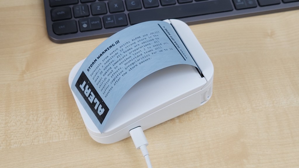
Mockup storm warning
We want Strandfall to be a highly physical experience that taps into the pleasure and exhaustion of movement, but we’re also mindful about accessibility. Ideally, every player will feel they have something vital and unique to contribute, not just the most athletic.
We also want Strandfall to incorporate role play. Just because everyone is part of the same expedition doesn’t mean they don’t want different things, or go about things in their own way. Hopefully we can give players the “alibi” to try out roles different from their normal selves, more courageous or argumentative or deferential. Since Alex and I haven’t designed larps before, we’ve brought on board veteran Nordic larp and RPG designer Juhana Pettersson as a consultant.
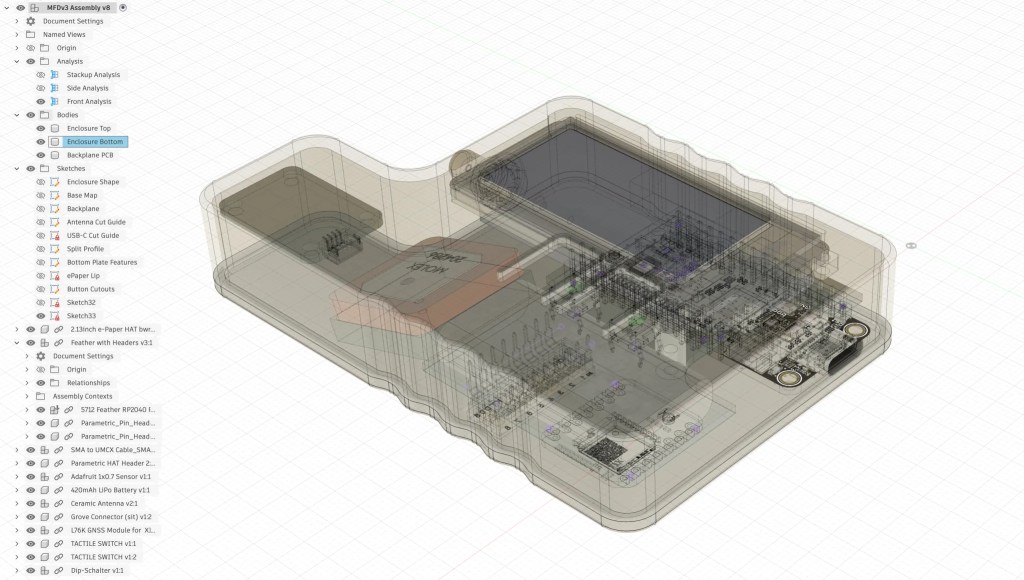
Wireframe design
While Strandfall is debuting in Edinburgh, it’s a site-responsive experience, not site-specific. It would be fairly straightforward to adapt it to other outdoor spaces and increase its duration and player count. Even though we don’t intend for Strandfall to be played by millions of people – its custom hardware and unique demands prevent that, plus we have more than enough of those games already – we have plenty of ideas of how to add depth and complexity to make it into a highly repeatable and extensible experience.
Before any of that, we have to pull off our first three-hour run in September. It’ll be free to participate, and you can find out more details and follow along on our website – we already have posts up about our influences like Death Stranding and PUBG, the technology and capabilities of our MFDs, and what I learned from this year’s Nordic Larp conference.
Our Approach to Bioresilience: Isomorphic Labs and Google DeepMind
AI is also a critical tool for our response.
The global biosecurity landscape is rapidly evolving. Shifting natural ecosystems, global travel and the potential misuse of AI require greater vigilance — yet AI is also a critical tool for our response. We need frontier AI models, and the scientific advances they will enable, to respond to these challenges and help make society more resilient to events like future outbreaks.
Today, Google DeepMind and Isomorphic Labs are sharing our joint approach to bioresilience.
Our work is twofold - to prevent threat actors from misusing our models, and to ensure that governments, scientists, biosecurity experts and our teams can harness these technologies to build a more resilient world.
Over the past 12 months, we have advanced more than 15 partnerships with government bodies, biosecurity organizations, and research groups to prevent threat actors from misusing our models, detect new outbreaks quickly and respond quickly and effectively.
Inside our bioresilience program
We believe society must harness AI’s advancing capabilities to address infectious diseases and prepare for future outbreaks.
Breakthroughs like Google DeepMind’s AlphaFold, which mapped the 3D structures of nearly all known proteins; Isomorphic Labs’ AI-powered Drug Design Engine (IsoDDE), which provides the real-world accuracy required to navigate novel biological systems with unprecedented precision; and AlphaGenome, which sheds light on genome function, are radically shifting the balance. Instead of just reacting to natural outbreaks or safety risks, we can now use these intelligent systems to help researchers design proactive defenses, accelerate the discovery of therapeutics, and safeguard the global health ecosystem with greater speed and precision.
With this in mind, we are making our AI models and agents available to trusted partners to support progress across three key areas: prevention, detection and response. Here are some examples:
Prevent:
To ensure our models, like Gemini, are safe and useful to experts, we follow a four-step safety process: threat modeling, evaluations, mitigations and monitoring.
We partner closely with in-house biologists, security experts and external partners to understand potential threats, test our models against them and build in robust safeguards.
Additionally, we’re working on adapting our SynthID watermarking technology to biology, which could help DNA synthesis providers screen for potentially risky, AI-generated biological sequences.
Detect:
We are helping make pathogen surveillance more cost-effective. For example, our agent AlphaEvolve can optimize algorithms used for producing and analyzing metagenomic sequencing data, helping detect new outbreaks faster. This optimization allows for quicker and more accurate DNA analysis, making it cheaper to track diseases worldwide on a large scale.
We are also exploring how technologies like AlphaGenome and Protein Function annotation could be used to help detect and characterize pathogens from sequence data, identifying novel patterns and emerging threats faster than traditional methods.
Respond:
Building on the scientific impact of AlphaFold, we are granting trusted researchers access to Google DeepMind’s latest AI systems to help accelerate the design of vaccines and other countermeasures for both known and novel threats.
To support government bodies and non-profit organizations during novel outbreaks, Isomorphic Labs has established a focused unit to rapidly deploy its drug design engine to design medical countermeasures that could address both naturally occurring pandemics and potential risks arising from the misuse of advanced AI. Working in collaboration with governments and global health authorities to advance a diverse range of diagnostic and therapeutic strategies enables the Isomorphic Labs Drug Design Engine’s real-world impact for bioresilience.
This is a complex, long-term effort, and part of our broader approach to managing potential Chemical, Biological, Radiological and Nuclear (CBRN) risks, aligning with the proactive mitigations and rigorous evaluation protocols of our Frontier Safety Framework.
We are committed to working openly and collaboratively — with biosecurity labs, governments and the broader scientific community — to ensure AI is developed and deployed responsibly to help protect against one of society’s greatest risks.
To read more about our work and our call for new partnerships, see this full update on our approach.
The Isomorphic Labs Drug Design Engine unlocks a new frontier beyond AlphaFold
We have unlocked a new paradigm of predictive accuracy in understanding our biomolecular world.
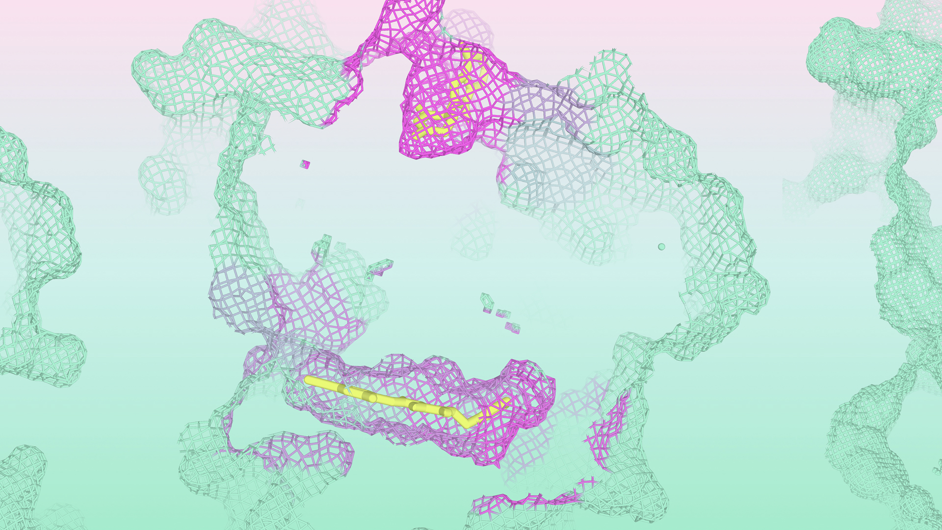
Today, we are excited to share an update on our progress towards a new frontier of drug design. We have unlocked a new paradigm of predictive accuracy in understanding our biomolecular world, allowing us to rationally design new medicines on a computer with unprecedented understanding and precision.
We are giving a glimpse at a subset of the powerful and expansive capabilities of the Isomorphic Labs Drug Design Engine (IsoDDE), a unified computational drug-design system, progressing beyond AlphaFold 3 (AF3) in its predictive accuracy and introducing new capabilities which bridge the gap between structure prediction and real-world drug discovery.
We demonstrate that our IsoDDE more than doubles the accuracy of AlphaFold 3 on a challenging protein-ligand structure prediction generalisation benchmark, predicts small molecule binding-affinities with accuracies that exceed gold-standard physics-based methods at a fraction of the time and cost, and is able to accurately identify novel binding pockets on target proteins using only the amino acid sequence as input.
IsoDDE offers a scalable foundation for AI drug design, providing the predictive fidelity required to navigate novel biological systems with unprecedented accuracy.
Since our release of AlphaFold 3 in 2024 together with Google DeepMind, the field of AI drug discovery has moved at an extraordinary pace. Whilst AlphaFold 3 delivered a dramatic leap in performance from previous generations of structure prediction models, a key challenge remained: understanding biomolecular structures alone was not sufficient for unlocking real-world drug discovery programs in silico (on a computer).
Progress in rational drug design - vital for solving human disease - requires highly accurate predictive models, across an expansive range of biochemical properties and interactions, that are able to work in concert with one another. Crucially, with so much of biological and chemical space still unexplored, these models need the ability to generalise their predictive power beyond their training sets to novel, unseen systems.
As we continue to address these challenges, we are excited to introduce the Isomorphic Labs Drug Design Engine (IsoDDE), and to preview a subset of IsoDDE's capabilities below and in our technical report.
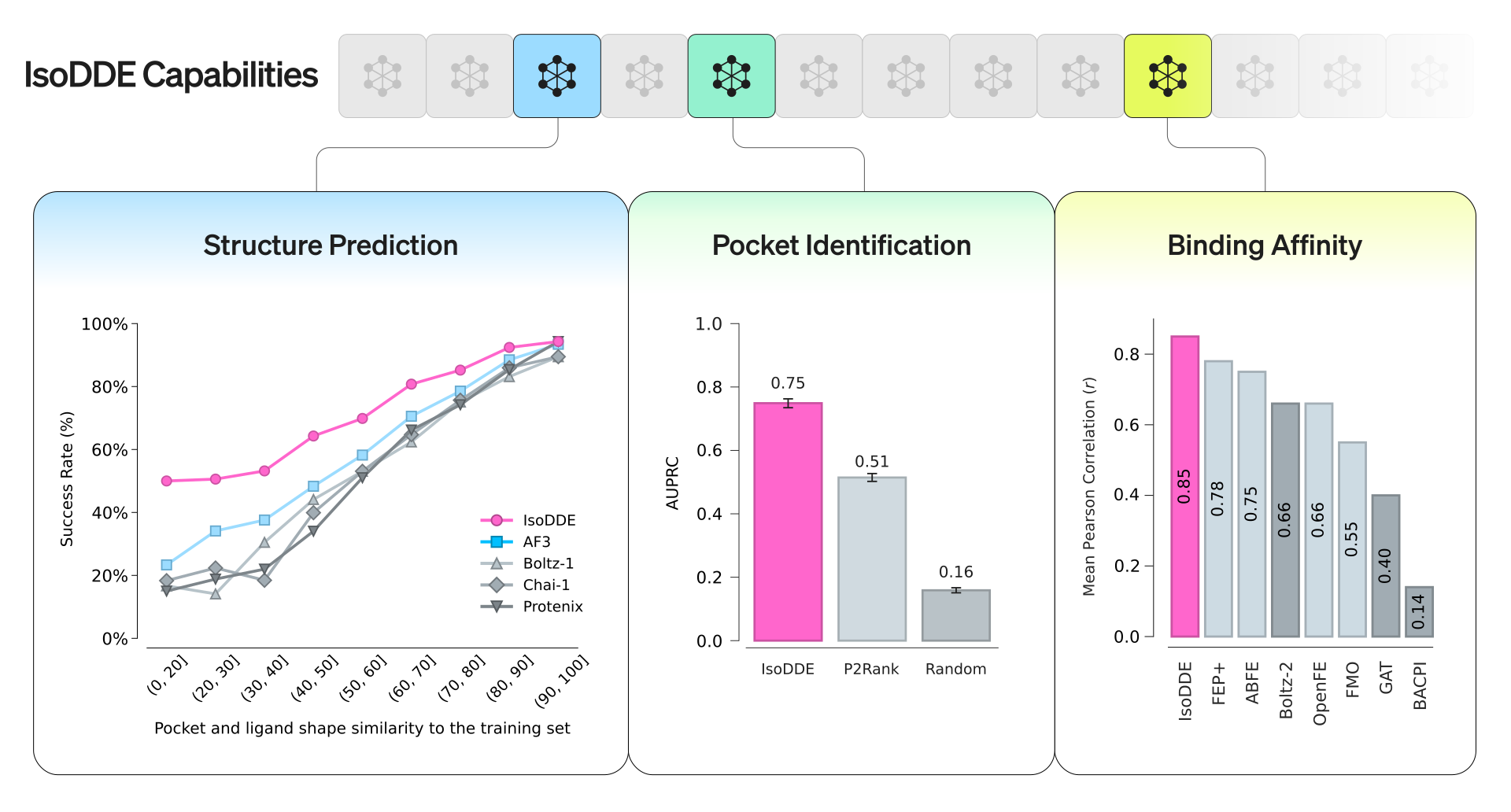
Structure Prediction of Truly Novel Systems
Accurately predicting the structure of biomolecules and how they interact remains a crucial capability for rational drug design. Many critical downstream tasks are unlocked by being able to accurately model the small nuances in a protein’s geometry - whether understanding the impact of disease-causing mutations, or predicting which molecules will bind to a target protein.
AlphaFold 3 transformed protein-ligand structure prediction at the time of its release and the freely available AlphaFold Protein Database accelerated science on a scale that was previously unimaginable. To date, it has been used by over 3 million researchers in more than 190 countries.
Benchmarks have subsequently revealed that there remained a gap in accuracy for structures that were dissimilar to the examples AlphaFold 3 had been trained on. In other words, that it can struggle to generalise to unexplored regions of biomolecular space where some of the biggest challenges and opportunities in drug discovery lie.
IsoDDE demonstrates a step change in the ability to generalise to protein-ligand structures that are highly dissimilar to those in its training set.
On the 'Runs N' Poses' benchmark (Škrinjar et al. 2025) - designed specifically to test generalisation to novel pockets and ligands - IsoDDE more than doubles the accuracy of AlphaFold 3 on the most difficult systems.
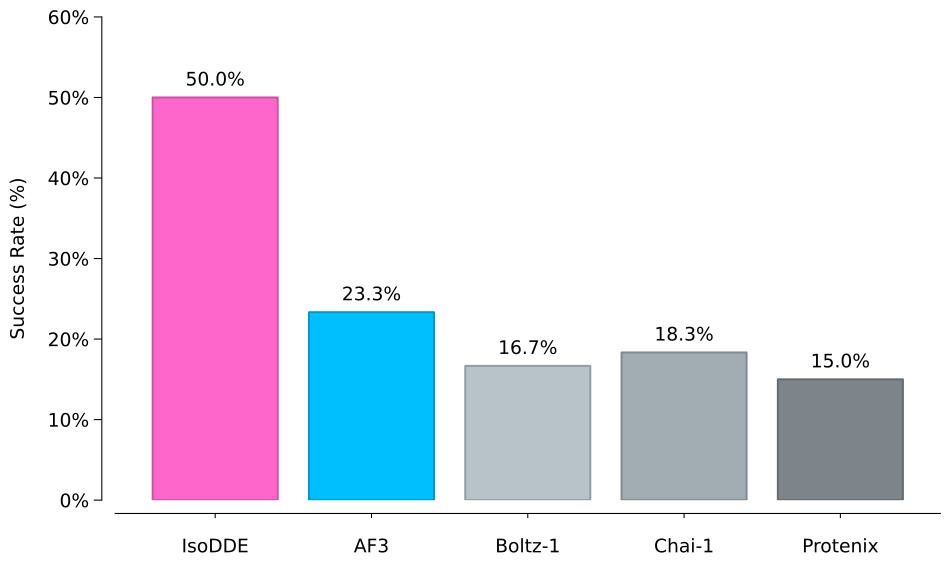
Protein-ligand structure prediction accuracy on hardest generalisation category ((0-20])- most dissimilar to the training set - from the 'Runs N’ Poses' benchmark
In the report, we demonstrate through several examples that we can successfully model complex, out-of-distribution events such as induced fits (where a protein adapts its shape to accommodate a bound ligand) and the opening of cryptic pockets (those hidden in the absence of a bound ligand) - critical biological mechanisms - even when these systems are distant from the training sets of such models.
IsoDDE is able to successfully predict the structure of a protein-protein interaction inhibitor bound to a cryptic pocket on the NKG2D homo-dimer interface (8EA6) from the lowest 0-20 similarity bin of the Runs’n’Poses test set (AlphaFold 3 fails on this example)
Opening a New Window for Complex Biologics
But small molecules (like aspirin) are only one piece of the puzzle. As therapeutic modalities expand toward complex biologics (like insulin), the ability to accurately model antibody-antigen interfaces is paramount.
IsoDDE provides a step change in accuracy for this domain. It outperforms AlphaFold 3 by 2.3x and Boltz-2 by 19.8x in the high-fidelity regime (DockQ > 0.8) on a challenging, novel antibody-antigen test set.
Crucially, IsoDDE shows remarkable performance on the CDR-H3 loop - the most variable and difficult part of an antibody to predict - effectively unlocking new possibilities for de novo antibody design.
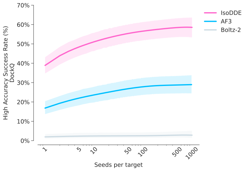
Antibody-antigen structure prediction accuracy for a challenging, low-homology test set (𝑛=334), showing the fraction of high-quality predictions at the protein interface (DockQ >0.8) as inference-time compute is increased. IsoDDE outperforms AlphaFold 3 by 2.3x and Boltz-2 by 19.8x
A New Gold-Standard for Binding Affinity Prediction
Knowing the 3D structure of a biochemical system is only the first step; effective drug optimisation requires knowing how strongly a molecule will bind to its target.
Traditional approaches are either limited to chemical space similar to the training data or by their high computational cost and difficulty of execution (e.g., physics-based approaches). Deep-learning based methods have more recently emerged that bring new speed to this task, but still lag behind physics-based approaches for accuracy.
IsoDDE surpasses all deep-learning methods by a considerable margin on three public benchmarks - FEP+ 4, OpenFE, and the recent CASP16 blind binding affinity prediction task.
In fact, remarkably, IsoDDE can surpass the performance of physics-based methods such as FEP, despite the fact that these require grounding in experimental crystal structures and IsoDDE does not.
By delivering highly accurate binding affinity predictions at speed, IsoDDE allows researchers to rapidly rank and optimise potential molecules across diverse chemical series during drug design programs.
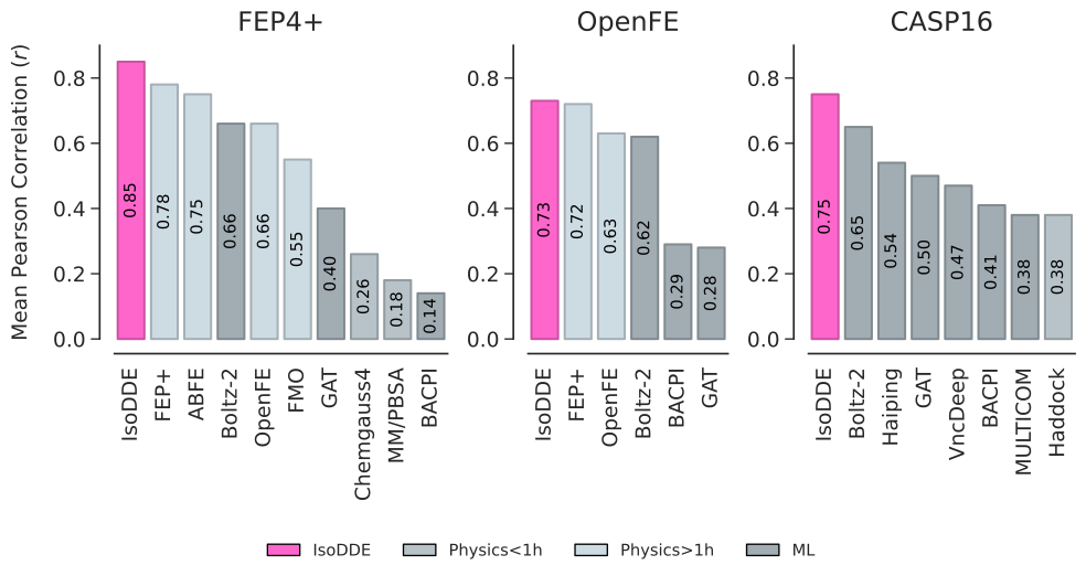
Binding affinity prediction performance across a range of public benchmarks
Expanding the Ligandable Proteome
The ability to identify all of the potential pockets on a protein, in the absence of a known ligand, unlocks a number of unique opportunities. Whether dealing with a first-in-class drug discovery target lacking structural annotation or pursuing a novel way to modulate a well-studied protein, a general pocket identification capability can be used to reveal the full set of possible mechanisms of action to pursue for molecular design.
IsoDDE exhibits the capability to identify novel, ligandable pockets even in the absence of a known ligand and far from the model’s training set. This capacity for ‘blind’ pocket identification demonstrates performance levels approaching experimental techniques like fragment-soaking which require large investments in time, significant cost and real-world experimental work. In comparison, IsoDDE runs on a computer in a matter of seconds.
We can see the power of this capability in the example of cereblon - a substrate receptor for the CRL4 E3 ligase complex - which plays a key role in tagging damaged or misfolded proteins for proteasomal degradation. For the last 15 years, it was believed that there was one principal way to drug cereblon: through the classic thalidomide-binding pocket. However, a recent study (Dippon et al. 2026) experimentally discovered a novel binding pocket that was both allosteric (away from the traditional binding site) and cryptic (hidden in the absence of a binding ligand).
IsoDDE was able to recapitulate the discovery of this pocket, predicting the location of both the known and the novel cryptic sites using only the sequence of cereblon as input, without specifying the identity of the ligands. Further, once the ligands were specified, IsoDDE was able to correctly fold them into their respective pockets in the correct orientation.
IsoDDE was able to recapitulate the recent discovery of a novel cryptic site on cereblon (Dippon et al., 2026) predicting the location of both the known and the novel cryptic sites using just the sequence of cereblon as input, without specifying the identity of the ligands.
Advancing Drug Discovery
IsoDDE represents a leap forward in accuracy and capability, bringing deeper understanding to the molecular machines that make up the human body, and advancing the process of designing drugs to modulate them.
Our dedicated drug design teams at Isomorphic Labs are using these capabilities every day across our programs – to understand unseen structures, identify uncharacterised pockets, and create novel chemical matter in the pursuit of new medicines for patients.
We look forward to continuing to push the frontiers of in silico drug design and bringing our new, more powerful capabilities to bear on historically challenging drug targets.
We thank our friends at Google DeepMind for productive discussions and collaboration.
Please use the following citation if you reference this work:
@manual{isodde2026,
  title = {Accurate Predictions of Novel Biomolecular Interactions with IsoDDE},
  author = {Isomorphic Labs Team},
  month = feb,
  year = 2026,
  doi = {10.5281/zenodo.19699685},
  url = {https://zenodo.org/records/19699685},
}
EU ban on destruction of unsold clothes and shoes enters into application
Under the new rules, businesses must prioritise keeping products in use by selling them or preparing them for reuse.

© jaturunp | Getty Images
From 19 July, large companies across the EU are prohibited from destroying unsold clothes, clothing accessories and footwear. Medium-sized companies will be subject to the same rules from 2030.
The measure, introduced under the Ecodesign for Sustainable Products Regulation (ESPR), aims to prevent the waste of valuable products and the resources used to make them.
When new, usable goods are discarded, the raw materials, water, energy and labour invested in their production are lost, while their disposal generates avoidable greenhouse gas emissions. By encouraging reuse, repair and more resource-efficient business practices, the new rules support the transition to a more circular and competitive European economy.
What the new rules mean for companies
Under the new rules, businesses must prioritise keeping products in use by selling them (including through discounts or alternative markets), donating them to charities or social enterprises, or preparing them for reuse (repairing, refurbishing or remanufacturing).
Destruction will be allowed only under specified circumstances and must be carried out in accordance with the waste treatment hierarchy, giving priority to recycling.
When the ban does not apply
Companies may only destroy unsold clothes and shoes in limited cases, such as when items are unsafe or damaged, counterfeit or infringing intellectual property rights, or are rejected by charities or donation schemes.
To prevent misuse, businesses relying on these exemptions must provide proof (e.g. documents or test results) and publish annual reports on what they have discarded.
How the rules will be enforced
National authorities will check compliance and can impose fines for violations. Companies must keep records for five years to allow inspections.
To reduce paperwork, businesses will use existing customs and logistics codes when reporting. Small and micro-businesses are exempt from these requirements.
Background
The Ecodesign for Sustainable Products Regulation (ESPR), which came into force in 2024, sets EU-wide rules to make products more durable, repairable, recyclable and resource-efficient.
The ban on destroying unsold textiles is one of the first concrete measures under the ESPR. Textiles are the first product group subject to this ban due to the negative environmental impacts of current business models, which often lead to the destruction of unsold goods.
According to the European Environment Agency, an estimated 4-9% of all textile products put on the market in Europe are destroyed before use, amounting to between 264,000 and 594,000 tonnes of textiles destroyed each year.
The Commission developed the rules after wide consultation with businesses, NGOs and experts to ensure they work in practice without creating unnecessary red tape.
More information
Ecodesign for Sustainable Products Regulation | European Commission
An Update on Igalia's Layer Based SVG Engine in WebKit (Reducing Layer Overhead)
The engine landed in WebKit and it works well, but it is still not the default.
Conditional layer creation in the layer based SVG engine
The last time I wrote here about the layer based SVG engine (LBSE) was back in autumn 2021, when I published the technical design document. A lot has happened since then, but maybe not what you would expect after almost four years. The engine landed in WebKit and it works well, but it is still not the default. You have to switch it on by toggling a runtime setting (in MiniBrowser). Between autumn 2021 and late 2022 LBSE was bootstrapped upstream, patch after patch. We added support for all the individual building blocks that make up SVG: paths, shapes, text, polygons, etc. within the new LBSE design. After that first big push the work stalled for a few months and resumed in mid-2023, and lasted until April 2024, due to generous support by Wix. During that period most advanced painting features, such as clipping, masking, filters, non-solid paint servers (patterns, gradients), markers, etc. were all implemented, sharing the logic with HTML and CSS rather than running through the separate code paths, as the legacy SVG engine did. Then the work paused again. A project of this size needs sustained funding to move forward, and for a while that funding was not there.
LBSE is promising, but it still has to earn its place, and it is worth being precise about what that means, because the goal was never simply “make SVG faster”. The legacy SVG engine is an island: historically grown, it has its own painting code, its own handling of transforms, clipping, masking, etc. and it shares only a little of the code that renders HTML and CSS for historical reasons. Many improvements that went into WebKit, went into “the other engine”, the main part, the HTML/CSS rendering engine. GPU-accelerated transforms and animations, accelerated compositing, all the work that made HTML/CSS fast. SVG sat right next to it and got none of it. That is what LBSE is really about. Put SVG on the same machinery, and it inherits all of that at once, and it keeps inheriting whatever comes next, instead of someone having to build it a second time for SVG alone.
The catch is that shared machinery is general machinery, and generality is not free. The legacy engine has been hand tuned for exactly one job, with two decades of tuning behind it. LBSE, on the other hand, has to integrate surgically into the shared HTML/CSS rendering code, without regressing that code even a little. This is the hottest code in the engine and it renders every web page out there, so sprinkling SVG special cases through layout and painting until LBSE looks good is simply not an option. Whatever LBSE needs either fits the existing design, or it has to make the existing design better for HTML and CSS too.
There is a second kind of work hiding in there as well. Some things that are rare in HTML are everywhere in SVG. Transformations are the obvious example. A typical web page has a handful of transformed elements, while in SVG almost every single element can carry a transform, and deeply nested transforms are the norm rather than the exception. The shared code was written with HTML in mind, and it does its job perfectly well there. So parts of the shared machinery have to be reworked, and fast paths that nobody ever needed for HTML have to be invented from scratch, without making anything slower for HTML in the process.
So the bar is a double one. LBSE first has to be competitive with the legacy engine on the plain, everyday rendering that legacy is already good at, because nobody switches engines if a static icon that never moves suddenly takes longer to paint. The rest, the hardware acceleration and every future improvement to the HTML/CSS engine that SVG now gets for free, only counts as a win once that first bar is met.
Fast forward to early 2026: This year the status quo finally changed. Igalia made a one-off investment into a fresh round of LBSE development, to give the engine the chance to prove itself. We are hopeful to finally show the world that LBSE is performant, and to attract new partners who share our vision that a performant, hardware-accelerated SVG engine is the future for UIs on embedded devices. This is the first of two posts covering the first half of 2026, where we stand now and how the LBSE project evolved since the long break in 2024. The last six months were intense, and ended with the single most invasive change to LBSE since it was first written. This post covers that change, and the next one picks up the hard problem it left behind.
A quick reminder of where we were#
When we designed LBSE, the central idea was simple. Instead of keeping the old, separate SVG painting code, SVG should reuse the very same machinery that HTML and CSS already use, the RenderLayer tree. That is what unlocked hardware-accelerated transform animations, perspective transformations, z-index support - all the nice things SVG never had before in WebKit.
To get there quickly, we took a shortcut in the early days. Every single SVG renderer got its own RenderLayer. A <rect>, a <path>, a <g>, everything. The reason was convenience: if every element has a layer, then the existing layer tree already knows how to order children, apply transforms, clip and composite. We did not have to reinvent any of that. Furthermore, the intrinsic SVG paint order, which follows the DOM structure 1:1, is guaranteed automatically this way, while z-index support is still there to deviate from that order when desired. All of that just works out of the box once every renderer receives its own layer. RenderSVGModelObject::requiresLayer() simply returned true all the time, and the rest of WebCore did the heavy lifting.
We knew from the start that this approach would most likely never ship in this form, because it is simply too wasteful. But that was fine. It was never meant to be the final design. What it gave us was a way to finally try out the things SVG had been missing for years, all running through the same machinery as HTML and CSS. It also gave us the possibility to reimplement all SVG render tree classes, in a way that’s fully unified between HTML and SVG, so that e.g. an SVG <clipPath> applied to an SVG element or an HTML element would no longer run through different code paths, as it historically did in WebKit. Thus just maintaining a 1:1 correspondence between renderers and layers was the fastest path to seeing the idea actually work, and once we had, the real shape of the engine could follow.
Correctness first#
When we resumed work on LBSE, we first had to make sure the engine worked again properly after the long pause of upstream work. LBSE received no testing during that period, so it was likely to be in a broken state, and that turned out to be the case. Text rendering was initially fully broken, most testing baselines were outdated, many new regressions were present, where the legacy SVG engine received fixes but LBSE did not. It took us a while to recover.
Rob Buis, my partner in the endeavor to bootstrap LBSE, did a lot of this work, so I could focus on attacking the remaining performance problems, profiling the engine, and trying new designs. We fixed a pile of crashes, for example in getBBox on <use> elements, in paths with NaN coordinates and line caps, and in markers whose children change. We fixed real rendering bugs too, including text not rendering at all, text opacity, gradients with a non-invertible gradientTransform, and support for SVG view fragments.
Filters got a lot of attention through spring. We made invalid filters behave like they do for HTML instead of dropping the element entirely, fixed feOffset clipping, filter scaling, and a convolution filter test. The most important filter change, though, has not landed yet. Once conditional layer creation, the change the rest of this post is about, removes the intermediate layers, a filter’s coordinate space no longer lines up with what the painting code assumed, and a lot of filtered content ends up in the wrong place. A pending pull request corrects that for non-layered renderers and clears a large batch of filter test failures under LBSE once conditional layers are enabled.
None of this is glamorous, but it is the foundation. With the engine behaving well again, we could finally go after the thing this whole effort was about.
The real goal, performance#
The point of LBSE was always performance. It was designed to unlock hardware-accelerated animations, which can potentially run much faster than in the legacy engine, since re-layouts and re-rasterization can be skipped entirely as the compositor is responsible for applying those transformations to the already-rasterized content. The catch is that scenarios which deliberately avoid that fast path suffer instead from the overhead of a layer per element. The benchmark we measure ourselves against here is MotionMark, and in particular its Suits subtest. Suits adds a large number of SVG primitives (rects and paths) that are clipped via <clipPath> elements, and animates them by modifying the transform attribute of each shape programmatically, in a requestAnimationFrame driven setup. It measures how many of them the browser can keep moving smoothly, which makes it a demanding, honest test of the SVG pipeline.
And here our early shortcut came back to bite us. Remember, every SVG renderer had its own RenderLayer. On a scene with thousands of shapes, that means thousands of layers. Each layer costs memory, and worse, each layer takes part in a lot of per-frame bookkeeping. Position updates, z-order lists, transform updates, repaint walks. None of these shapes should actually need a layer - a path/rect with a plain 2D transform is the most ordinary thing an SVG can contain. Yet we paid the full layer price for every one of them.
So the way forward was clear: stop giving every renderer a layer, and create one only when an element actually needs it. The first focus is transformed elements, the plain shapes that carry nothing but a 2D transform. Clipped elements keep their layer for now, and dropping that one too is future work. In Suits this first step already removes the layer from every transformed path, leaving only the clipped rects and the <svg> root, as the diagram below illustrates.
Old: a layer for everythingNew: no layers for transformed elements<svg>defsgrad + clips<rect>clip-pathtransform<path>transform<rect>clip-pathtransform<path>transform…LLLLLone RenderLayer per shape, thousands of them<svg>defsgrad + clips<rect>clip-pathtransform<path>transform<rect>clip-pathtransform<path>transform…LLLlayers only for the clipped rects and the <svg> root
Suits builds a flat list of shapes directly under the <svg> root: alternating clipped <rect> elements and plain <path> elements, each with a gradient fill and a transform that is updated on every animation frame. A blue L marks a renderer that owns a RenderLayer. On the left every shape has one. On the right the plain transformed paths no longer do, while the clipped rects keep theirs for now, so only they and the <svg> root own a layer.
However, it turned out that we cannot easily remove layers for transformed containers, only for transformed leaf elements - we’ll get back to that later.
Conditional layer creation#
Pulling layers out from under the whole engine is risky, but the real reason we did not do it in one jump is that it would have been a huge, unreviewable patch, since a lot of new concepts had to be invented first. A string of preparation patches had to land instead, each one dormant on its own, so that the eventual switch to conditional layers had solid ground to stand on.
The groundwork was mostly about finding a new home for the things that used to live on the layer. A RenderLayer carried a pile of SVG-only fields that non-SVG layers never need, so we moved them into a lazily allocated SVGData struct that only exists for layers within an LBSE subtree. That was a good cleanup on its own, and everything else built on top of it, starting with the transform. We used to cache an element’s local transform on its RenderLayer, and with no layer we needed a different place to cache it, rather than recomputing it on every use. So we did what the legacy SVG engine had done all along and cached the transform on the renderer itself, with a m_localTransform member and an updateLocalTransform() method that plays the same role the layer version used to. A couple of follow-up patches (311763@main and 315597@main) then made sure dynamic transform updates work for both layered and non-layered SVG renderers.
With the SVG data and the transform moved into their new homes, we built a DOM-order paint path for non-layered SVG children, followed immediately by the matching DOM-order hit-test path. Behind both sits an SVG-specific, DOM-order collection of the renderable children, and it plays a crucial role in making conditional layer creation work at all.
HTML and SVG behave differently here. Take a block with three <div> elements where the middle one carries a CSS transform. The transform makes that middle element establish its own stacking context, so it no longer paints in place. The paint order becomes the first div, then the third, and only then the transformed middle one on top, assuming it has a non-negative z-index. For SVG that would be wrong. SVG content has to paint in strict document order, whether or not a layer is involved, so the middle child still paints between its two siblings. Adding z-index support so SVG can deviate on purpose is a separate issue. None of this had to be solved by hand when every renderer had a layer and the layer tree sorted everything for us. With conditional layers, and a mix of layered and non-layered children, we now have to guarantee that document order ourselves.
Both paths were gated behind a check that still saw a layer on every renderer, so they had no effect yet and stayed inactive until conditional layers turned them on. Next we taught non-layered transformed content to position itself correctly inside the paint recursion, folding the transform of a shape, image or piece of text into the coordinate system during painting. And just before enabling conditional layers, we landed a large batch of tests for the tricky mixed cases, so any regression from the coming change would surface right away. There is also an internal flag, LayerBasedSVGEngineForceLayerCreationEnabled, that brings back the old behavior, and it was a great help for bisecting problems, because it lets you compare the two worlds side by side.
With all of that in place, we could finally flip the switch. The headline change, conditional layer creation, landed in June 2026. The idea is to create a RenderLayer only when an element needs one for an intrinsic reason. Each renderer now implements a new method, requiresLayerForSVGIntrinsicReasons(), and its return value alone decides whether that renderer gets a layer. An SVG element gets a layer only when some painting effect needs the extra machinery a layer provides. That means opacity groups, clipping, masking, filters, blend modes, and isolation. A 3D transform needs one too, along with a handful of related properties like perspective, preserve-3d, and an explicit z-index. Everything else, the vast majority of shapes and groups, gets no layer at all.
Plain 2D transforms need a bit more care. On a leaf element like a shape or a piece of text, a 2D transform no longer forces a layer of its own. We store the transform on the renderer and fold it into the coordinate system at paint time, concatenating it onto the current transformation matrix just before the element draws. The exception is a transformed container, which still keeps its own layer. The compositing logic is built around the layer tree, not the render tree, and expects every transformed container to have one, because it computes a composited element’s current transformation matrix (CTM) by walking up the chain of ancestor layers and concatenating their transforms. A transformed container without a layer would drop out of that walk, so its transform would be lost and the composited descendant would be left with the wrong CTM. Reworking that expectation would be a substantial effort, so for now we settled on a compromise and keep a layer for every transformed container, which at least guarantees that an element’s ancestor chain transformation can be correctly computed.
With conditional layer creation in place, LBSE can now decide, renderer by renderer, whether a layer is needed at all, and create one only where an SVG renderer genuinely requires it. For non-composited content this is exactly what we wanted. The transform folds straight into the paint recursion, the shape draws in the right place, and no layer appears. Composited content, though, is now broken. As soon as a single composited element sits among plain, layer-less siblings, the strict SVG paint-order contract falls apart. The compositing code path can only order content that owns a layer, and now that conditional layer creation has taken layers away from most of the tree, it can no longer keep that composited element in its correct document-order slot.
We won the fast common case and lost the composited one in the same move, and winning it back without undoing all of this is the hard part the next post is about: the interesting compositing problem, and the design that finally solved it.
Let me close with a huge thanks to the Apple developers, involved in validating the LBSE work: thanks Simon, Said, Karl and Ahmad for the insightful discussions and input how to move LBSE forward! Thanks for reading until the end :-)
That's the Front for Today
Issue No. #260718 — Saturday, July 18, 2026 — went to press 2026-07-19 at 06:41 UTC.
About This Magazine
The Daily Front is a daily digital magazine assembled from the stories that reached the front page of Hacker News on Saturday, July 18, 2026. Headlines, points, and comment counts are recorded as they stood at press time. All articles remain the property of their original authors — every piece links back to its source and its discussion thread.
How It Was Made
Fetched, cleaned, and typeset by an automated pipeline. An editor model laid out the pages, chose the highlights, and briefed the cover illustrator — 24 model calls and 171k tokens in total. Set in Jacquard 12, Playfair Display, Source Serif 4, and IBM Plex Mono, all served via Google Fonts under the SIL Open Font License.
The Cover
The cover illustration was commissioned with this prompt:
A dreamlike Byzantine mosaic meets cyber-folk tapestry: an unattended desktop monitor shines like a cold altar while tiny silver mechanical hands offer plain sealed software parcels into its side; a translucent analytical automaton floats above a patterned table, arranging jewel-toned geometric tiles into a silent proof; abandoned help-desk chairs rest beneath a collapsing graph formed from gold-thread lines and dark enamel dots; a small home camera leaks glowing map-pin shapes across the floor like scattered votive flames. Intricate tessellated surfaces, hand-laid glass tiles, woven fiber texture, iridescent highlights, flattened ceremonial perspective, deep ultramarine, oxidized copper, pearl white, and ember red accents, mystical yet technical atmosphere, no text, no letters, no numbers, no logos, no signage.
Production Ledger
| Stage | Model | Calls | Tokens In | Tokens Out |
|---|---|---|---|---|
| extract | gpt-5.5 | 23 | 105,502 | 44,557 |
| layout | gpt-5.5 | 1 | 16,628 | 4,433 |
Credits & Contact
All content — articles, posts, comments, and the images within them — belongs to its original authors and is reproduced here to point readers back to the source. Full credit goes to those creators; every item links to its original and its Hacker News discussion.
If you are an author and would like your content removed from an issue, write to hi@johnnys.page and it will be taken down.
Feedback is always welcome at the same address: hi@johnnys.page.
Credit where credit is due.
Every page of this issue began as someone else's work — these are the original sources, linked in full.
- LG monitors silently install software through Windows Update without consent
- GPT-5.6 used a prompt to close a 30-year gap in convex optimization
- Regressive JPEGs
- What AI did to stackoverflow in a graph
- The Kimi K3 Moment
- Fable 5 vs. GPT-5.6 Sol on an NP-Hard Problem: Does /goal help?
- Setting up your spare Mac for Claude Code to control, a step-by-step guide
- Why do AI company logos look like buttholes? (2025)
- TP-Link Kasa cameras leaked home GPS via unauthenticated UDP for 6 years
- Qubes OS Security in the Public Record
- In-toto: A framework to secure the integrity of software supply chains
- Speech Recognition and TTS in less than 500kb
- Vāgdhenu: A Sanskrit Chanting TTS System
- Elixir-lang.org has a new design
- Gleam Is Now on Tangled
- Show HN: Q3Edit – Edit and play Quake 3 maps in the browser
- Stenchill: 3D Printable Solder Paste Stencil Generator
- I started a “dirt notebook”
- The Computer at the Bottom of a Canal
- Reviving a 15-year-old netbook with Arch Linux
- Is this the end of the once-mighty GoPro?
- A Second-Grade Teacher Revived a Beloved Video Game
- Lego building instructions through time
- Tech note: making your own V-I plots at home
- I'm Making Strandfall, a Solarpunk Orienteering Larp
- Our Approach to Bioresilience: Isomorphic Labs and Google DeepMind
- The Isomorphic Labs Drug Design Engine unlocks a new frontier beyond AlphaFold
- EU ban on destruction of unsold clothes and shoes enters into application
- If You Build It, They Will Come
- An Update on Igalia's Layer Based SVG Engine in WebKit (Reducing Layer Overhead)
Browse all issues in the archive →