Cover illustration

TheDaily Front

Issue No. 5 Monday, July 13 2026 #5 — MONDAY, JULY 13, 2026
Where ghosts haunt kernels, agents raid home folders, and the sea refuses to stay inside the chart.
Monday, July 13, 2026 The Daily Front No. 5 — Contents
30stories
10,853points
4,959comments
232kllm tokens
Assembled with 28 model calls — 165,379 tokens read, 66,928 written.

Highlights

GhostLock, a stack-UAF that has existed in all Linux distributions for 15 years

A 15-year Linux kernel bug arrives with a full exploit writeup, a container escape, and a bounty large enough to make every sysadmin sit up straight.

Ask HN: Add flag for AI-generated articles

HN debates whether AI-written articles deserve a warning label, and whether the old voting customs still hold in the new synthetic age.

Zig Creator Calls Spade a Spade, Anthropic Blows Smoke

A dispute over Zig, Rust, Bun, and Anthropic becomes the day’s loudest proxy war over marketing, engineering, and AI-era programming culture.

Grok CLI uploaded the whole home directory to GCS

Two Grok CLI posts raise the practical question every agent user must answer: what exactly did you just give permission to read?

A graph that should be front-page news

Climate data makes a double appearance: one alarming graph and one volunteer effort to preserve public climate resources.

From the Editor

This was a day for machines behaving badly and institutions being asked to prove their manners. The kernel had an old ghost in the rafters, the agents were rifling through the drawers, and the readers once again demanded labels on whatever prose the new mills grind out.

  1. GhostLock, a stack-UAF that has existed in all Linux distributions for 15 years3
  2. Ask HN: Add flag for AI-generated articles4
  3. Zig Creator Calls Spade a Spade, Anthropic Blows Smoke4
  4. Samsung Health app threatens data deletion if users opt out AI training4
  5. Grok CLI uploaded the whole home directory to GCS5
  6. Grok uploaded my user directory to xAI's servers5
  7. Telegram's t.me domain has been suspended5
  8. Building and shipping Mac and iOS apps without opening Xcode6
  9. Apple's new SpeechAnalyzer API, benchmarked against Whisper and its predecessor7
  10. A graph that should be front-page news8
  11. Former NOAA employees built Climate.us to preserve climate data and resources9
  12. LAPD lets contract with surveillance giant Flock expire10
  13. Sam Neill has died11
  14. The art and engineering of Sega CD Silpheed12
  15. Linux on the Sega 32X. Who needs hardware synchronization primitives anyway?13
  16. Designing and assembling my first PCB14
  17. Benchmarking 15 “E-Waste” GPUs with Modern Workloads15
  18. Show HN: I implemented a neural network in SQL16
  19. Show HN: DOM-docx – HTML to native, editable Word docs (MIT)17
  20. Backtrack-Free Cursive18
  21. The social physics of conversation: Communication patterns matter19
  22. Interrail: 6,379Km and 13 Countries over 7 weeks20
  23. TFTP Honey Pot Results21
  24. Cyberpunk Comics, Manga and Graphic Novels22
  25. A voxel Tokyo in real Japan time – ride the Yamanote line and study Japanese22
  26. Ancient Roman Board Game22
  27. Beavis Ultrasound PnP ISA Sound Card Replica23
  28. Show HN: YouTube Guitar Tab Parser24
  29. Are you telling me a readonly property is wrecking my performance?24
  30. GhostLock, a stack-UAF that has existed in all Linux distributions for 15 years25
The Daily Front Page 2 of 26
Monday, July 13, 2026 The Daily Front No. 5 — The Ghost in the Kernel
article

GhostLock, a stack-UAF that has existed in all Linux distributions for 15 years

by ranger_danger·▲ 414 points·194 comments·nebusec.ai ↗
Triggering the bug does not require any special kernel config or privilege.

GhostLock (CVE-2026-43499) is a Linux kernel vulnerability found by VEGA that exists in every major distribution since 2011. Triggering the bug does not require any special kernel config or privilege. By turning it into a 97% stable privilege escalation and container escape, Google has rewarded us $92,337 in kernelCTF. This writeup covers the technical details of the exploit.

Vulnerability Summary

GhostLock (CVE-2026-43499) lets an unprivileged local attacker:

  • Get a dangling kernel pointer to kernel stack memory with only regular threading syscalls.
  • Write a pointer to an almost arbitrary address.
  • Hijack a function table to get control flow hijack and eventually get root access.

GhostLock was introduced in Linux 2.6.39 and fixed in Linux 7.1. It has existed in the Linux kernel for more than 15 years. Every Linux distribution without the patch is affected and should consider upgrading to the latest LTS version.

Vulnerability Analysis

Overview

GhostLock was introduced with the rtmutex rework in 8161239a8bcc (“rtmutex: Simplify PI algorithm and make highest prio task get lock”), and sat untouched for about fifteen years until the April 2026 fix in 3bfdc63936dd (“rtmutex: Use waiter::task instead of current in remove_waiter()”). The affected range is v2.6.39-rc1 to v7.1-rc1, with CONFIG_FUTEX_PI=y the only requirement and no capabilities or user namespaces needed.

remove_waiter() in kernel/locking/rtmutex.c clears current->pi_blocked_on. That is correct on the normal slow path, where current is the task that owns the waiter. It is wrong on the proxy path. rt_mutex_start_proxy_lock() enqueues, and on error rolls back, an rt_mutex_waiter on behalf of another task, so current is the requeuer rather than the waiter.

The waiter object lives on the stack of a task sleeping in FUTEX_WAIT_REQUEUE_PI. A FUTEX_CMP_REQUEUE_PI then proxies that waiter onto the target PI futex. When the rtmutex chain walk reports a deadlock, the rollback dequeues the waiter from the lock but clears pi_blocked_on on the requeuer. The waiter task keeps pi_blocked_on pointing at its own stack frame, which is popped the moment the waiter returns to userspace. Any later PI chain walk through that task follows the dangling pointer.

Root cause

Like other lifecycle bugs, this occurs when a function is used by a caller it was never designed to support.

The helper function remove_waiter() was originally written for exactly one scenario: a thread blocks on its own, then cleans up after itself. So it has always assumed that current (whichever thread happens to be running) is the waiter it needs to clean up, and clears current->pi_blocked_on accordingly.

However, Requeue-PI breaks that assumption. Through rt_mutex_start_proxy_lock(), this helper is now used to clean up on behalf of a different, sleeping thread. In that path, current is the thread that issued FUTEX_CMP_REQUEUE_PI rather than the actual waiter.

When __rt_mutex_start_proxy_lock() returns -EDEADLK, it rolls back via remove_waiter(), the misused helper.

int __sched rt_mutex_start_proxy_lock(struct rt_mutex_base *lock,
                                      struct rt_mutex_waiter *waiter,
                                      struct task_struct *task)
{
  int ret;
  raw_spin_lock_irq(&lock->wait_lock);
  ret = __rt_mutex_start_proxy_lock(lock, waiter, task);
  if (unlikely(ret))
    remove_waiter(lock, waiter);          // ret == -EDEADLK
  raw_spin_unlock_irq(&lock->wait_lock);
  return ret;
}

remove_waiter() then scrubs the wrong task.

static void __sched remove_waiter(struct rt_mutex_base *lock,
                                  struct rt_mutex_waiter *waiter)
{
  ...
  raw_spin_lock(&current->pi_lock);
  rt_mutex_dequeue(lock, waiter);
  current->pi_blocked_on = NULL;            // should be waiter->task
  raw_spin_unlock(&current->pi_lock);
  ...
}

waiter is the object that lives on the sleeping thread’s own stack, while current here is the thread that requested the requeue. The fix locks waiter->task->pi_lock and clears waiter->task->pi_blocked_on instead. This issue slips past lockdep, which only checks that a pi_lock is held but not whose it is.

Triggering the -EDEADLK Path. Reaching the -EDEADLK rollback needs a PI dependency cycle built from three futex words and three threads.

  • f_pi_chain, a PI futex, locked first by the waiter thread.
  • f_pi_target, a PI futex, locked first by the owner thread. This is the requeue target.
  • f_wait, the plain futex the waiter blocks on with FUTEX_WAIT_REQUEUE_PI.

The sequence is:

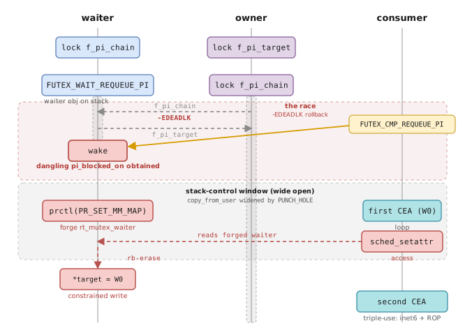
  1. The waiter takes f_pi_chain, then blocks in FUTEX_WAIT_REQUEUE_PI(f_wait -> f_pi_target). Its rt_mutex_waiter is now on its stack.
  2. The owner takes f_pi_target, then blocks on f_pi_chain, which the waiter holds.
  3. The main thread calls FUTEX_CMP_REQUEUE_PI(f_wait -> f_pi_target).
Race windowRace window

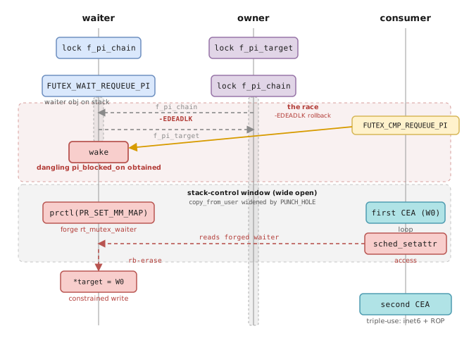
The requeue tries to proxy the waiter onto f_pi_target. The owner of f_pi_target is already blocked behind the waiter through f_pi_chain, so the chain walk closes the loop waiter -> f_pi_target -> owner -> f_pi_chain -> waiter. It returns -EDEADLK and takes the buggy rollback. The waiter wakes with a dangling pi_blocked_on.

Here the only ordering that matters is the requeuer rolling back the waiter while the waiter still owns the soon-to-be-freed object, and once the cycle is staged that happens on its own. After it resolves there is no time pressure at all. The waiter sits in userspace with a dangling pi_blocked_on, and the follow-up sched_setattr() that walks the chain can fire whenever it likes. The UAF window is wide open.

The catch is where the freed object lives on the kernel stack (stack-UAF if we call ret out of the futex syscall a “free”). To reclaim it, we need to find a syscall that can land controlled bytes back on the same stack at the same depth (offset).

Triggering the stack-UAF

Staging the three-futex cycle leaves the waiter task in userspace with pi_blocked_on dangling into its old FUTEX_WAIT_REQUEUE_PI frame. Everything below rides on that one pointer.

Note that three threads is for better understanding. To win the race and trigger UAF, you only need one CPU core.

The initial primitive from GhostLock

By now we hold a pointer into freed kernel stack, and we can trigger, at will, a kernel access that dereferences it as an rt_mutex_waiter. We can spray controlled bytes onto that stack and forge the rt_mutex_waiter outright. Depending on the layout we forge, this one access yields several primitives, two main ones:

  • write a pointer to an arbitrary (but constrained) address
  • write 8 bytes of zero to an arbitrary (but constrained) address

Several pointer dereferences and integrity checks run before the primitive fires, and after it fires the kernel returns normally, no crash.

So our main questions, each answered in a section below:

  • how do we get the freed stack memory back (spray)? -> Reusing the stack
  • how do we get the fake rt_mutex_waiter past its built-in structural checks, and forge pointers that read as valid? -> From fake waiter to a write
  • which write primitive, and what do we write where? what does the primitive constrain about the “arbitrary” address? -> Use inet6_protos

Exploit Details

Exploit Summary

  • prefetch -> Leak the kernel image slide and the physmap base.
  • GhostLock -> Leave a dangling rt_mutex_waiter in the waiter task’s pi_blocked_on.
  • (stack-)UAF Reclaim -> Use PR_SET_MM_MAP to reclaim the waiter’s own kernel stack and forge a fake rt_mutex_waiter over the freed frame.
  • Arb address writer -> Rtmutex rb-tree erase: one constrained pointer write (which we can reclaim its content), overwrite struct which contains a function table: inet6_protos[IPPROTO_UDP] = <CEA pointer>.
  • CPU entry area -> Host {fake inet6_protocol, pivot slots, ROP stack} all together at a known direct-map address.
  • Trigger CFH -> Trigger a loopback IPv6 UDP packet calls through the overwritten handler and pivots.
  • DirtyMode -> One write flips core_pattern’s mode bits, then the rest LPE is pure userspace.

What about Android?

This part we are focusing on basic exploit steps of generic x86 Linux systems, our next blog will discuss how to exploit GhostLock on Android, reclaiming stack frame, bypassing both ASLR and CFI.

Background of used tricks

Prefetch ASLR Leak

A prefetch on a given address runs in a different number of cycles depending on whether that address is mapped in the current page tables, so an unprivileged process can time prefetch across the kernel range and read off which addresses are mapped (the prefetch paper has the details).

It works here as Linux barely randomizes the base of its default kernel image (~9 bits of entropy for text base), so a little averaging can recover the KASLR base with near 100% reliability.

In theory any CPU with prefetch and without proper Kernel Page-Table Isolation is affected. But in practice it is more of an x86 technique (unless the ARM target runs KPTI off). kernelCTF images keep KPTI disabled.

kernelCTF images keep KPTI disabled, but even with KPTI on, prefetch paired with EntryBleed can still recover the kernel image base through the trampoline.

CEA spray and randomization bypass

The CEA (CPU entry area) is a per-CPU x86 structure holding the stacks and register context used for entry and exception handling: on an exception, interrupt, or syscall the CPU switches to a stack that lives in the CEA, and the entry code spills the register frame (pt_regs) there. An unprivileged userspace program can trigger a software exception and write its own register context into the pt_regs saved on a CEA exception stack. Before 6.2 the CEA sat at a completely fixed address, so we can place about 120 bytes of contiguous controlled memory at a known kernel address, which is very handy for forging structures, for absorbing the side effects of the pointer dereferences along the way, and for staging a ROP stack.

After Project Zero’s Bringing back the stack attack writeup, the kernel started strongly randomizing the CEA’s virtual address (since 6.2). But the virtual address of the CPU entry area is never needed, as the CEA’s physical offset is fixed, so its direct-map alias follows from the physmap base (same observation @kqx used).

That direct-map address is easy to leak with prefetch, plus candidate-edge normalization and a check against the predicted CEA page to reject neighbouring aliases. (The direct-map leak is noisier than the text one and may need a little more tuning, but it lands at very high accuracy on the target in the end.) So we can always compute the CEA’s other virtual-address mapping:

cea_direct = physmap_base + CPU1_CEA_BASE

Note that each CPU’s CEA virtual address is randomized to a different place. Their physical addresses are all fixed, though, and this offset depends mainly on the target’s kernel version and boot memory size. In the kernelCTF LTS 6.12.80 3.5G-boot environment, it is 0x11c517000(+0x1f58).

Reusing the stack: forging the waiter with PR_SET_MM_MAP

The dangling object is the waiter’s own stack rt_mutex_waiter.

struct rt_mutex_waiter {
  struct rt_waiter_node tree;     // rb node, lives in lock->waiters
  struct rt_waiter_node pi_tree;
  struct task_struct *task;
  struct rt_mutex_base *lock;
  unsigned int wake_state;
  struct ww_acquire_ctx *ww_ctx;
};

Controlled bytes have to land back over that exact frame, on the waiter thread’s own stack, and stay there long enough to be read. The waiter thread returns from the futex syscall and immediately calls prctl(PR_SET_MM, PR_SET_MM_MAP, ...). Inside, prctl_set_mm_map() copies a user-supplied auxv into a fixed-size unsigned long user_auxv[AT_VECTOR_SIZE] stack buffer. That buffer sits at roughly the same stack depth as the freed waiter, so it is a large, naturally-aligned, namespace-free block of controlled qwords landing right on top of the old object.

The auxv is laid out so the overlapping qwords become:

  • tree, an rb node crafted so erasing it promotes one chosen child pointer (W0_BASE, below) into the tree root.
  • task, set to &init_task, a valid task_struct so the chain walk’s task derefs are safe.
  • lock, set to &inet6_protos[IPPROTO_UDP] - 8, the write target.
  • wake_state, set to 0.

The auxv is backed by a memfd and positioned so the copy straddles a page boundary. A sibling thread races fallocate(PUNCH_HOLE) on the trailing page during the prctl, which stretches the copy_from_user window. The forged waiter stays live on the stack while, on another CPU, a consumer thread fires sched_setattr() on the waiter to walk the PI chain.
The race window is wide and we believe GhostLock is also exploitable on a single-core CPU.

clone/setsockopt/pselect/keyctl and other syscalls with large controlled stack locals work the same way. prctl is just convenient here. The buffer is large, aligned, and needs no namespace.
Here’s more useful syscalls that can reclaim the stack frame in our open-sourced PoC code.

From fake waiter to one controlled (limited) write

Controlling the waiter does not give an arbitrary write. The chain walk only does:

task->pi_blocked_on -> fake waiter
fake waiter->lock    -> fake rt_mutex_base
rt_mutex_dequeue(lock, waiter)        // rb_erase on lock->waiters

rt_mutex_dequeue() is an rb-tree erase, and erasing a single-child root writes that child into the root slot. Pointing lock at target - 8 lines the rt_mutex_base fields up over the data around the target pointer.

target - 8  ->  raw_spinlock_t wait_lock        (must read as "unlocked")
target      ->  waiters.rb_root.rb_node          (this slot gets written)
target + 8  ->  waiters.rb_leftmost
target + 16 ->  owner

The fake waiter’s rb node is crafted so the erase writes exactly one child pointer into rb_root.rb_node. The write primitive itself is a single constrained store: *(uint64_t *)target = W0_BASE.

The constraints are also highly strict: The qword before the target must read as an unlocked spinlock, meaning zero in the low 4 bytes, or the trylock fails and the walk exits without writing. The qwords after it (rb_leftmost, owner) must not steer the walk into an uncontrolled top waiter or owner. An unmapped value there faults and panics the box. The equivalent target address constraint is roughly as follows (*target will be written to a pointer):

*(u32 *)(target - 0x08) == 0
*(u64 *)(target + 0x08) == 0 // simplified
((*(u64 *)(target + 0x10)) & ~1ULL) == 0
// Then we can do:
*(u64 *)target = &W0->tree.entry  // W0_BASE

Here the W0_BASE has to point at something that stays valid through the comparisons and the no-owner wakeup later in the same rt_mutex_adjust_prio_chain(). We point it at the direct-map alias of the CPU entry area, which pays off twice:

  • Before the write: the CEA is controllable memory at a known address, so we can forge a self-consistent fake waiter and lock at W0 that survives the walk.
  • After the write: the target now points into the CEA. Once the walk is over, W0 no longer has to look like a waiter at all, so we can re-spray the CEA with whatever the kernel expects the target to point at (if we overwritten a function table pointer with W0, we can now fake function pointer in CEA to get Control Flow Hijack).

Why the CEA?

There’s several ways to spray controlled memory at a fixed (knowned) kernel address. The CEA is one of the more efficient, and its main limit is the ~120-byte small size. NPerm, kernelsnitch and other tricks can do the same job with more room.

Before the trigger, W0 is spraied as that fake waiter and lock pair: task = &init_task, a legit prio, and a lock whose wait_lock reads unlocked and whose owner is benign, so the dequeue, re-enqueue, priority update and wakeup all survive.

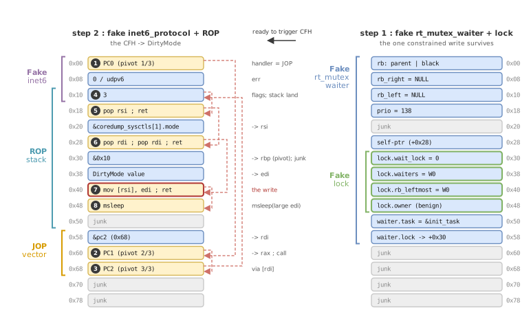
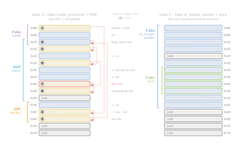
The following figure shows how CPU entry area is used to first hold fake rt_mutex_waiter and lock structures, then serve inet6 (next section), ROP stack and JOP gadgets for stack pivoting at the same time, and eventually use a very short ROP to perform the DirtyMode and safely halt the core.

Dual use of the CEA, with three data structures overlapped within 104 bytesDual use of the CEA, with three data structures overlapped within 104 bytes

Use inet6_protos[IPPROTO_UDP] to help

Start from now the exploit path would differ from targets, as of regular x86_64 Linux kernel, we can pick a shorter path by just overwriting some function table (or any object that contains one), as we already have KASLR leaked and ready to get a CFH.

A scan of writable data turns up many pointer tables whose neighbours satisfy the layout above. inet6_protos[IPPROTO_UDP] is a nice one. The neighbours fall out for free, and the trigger is a trivial unprivileged loopback packet.

inet6_protos[16]  == NULL              // fake wait_lock -> unlocked
inet6_protos[17]  == &udpv6_protocol   // <- target (IPPROTO_UDP)
inet6_protos[18]  == NULL              // fake rb_leftmost
inet6_protos[19]  == NULL              // fake owner

After the write, inet6_protos[IPPROTO_UDP] points into the CEA page, where the kernel expects an inet6_protocol.

struct inet6_protocol {
  int (*handler)(struct sk_buff *skb);
  int (*err_handler)(...);
  unsigned int flags;
};

So W0 is re-spraied as a fake inet6_protocol. handler is the first pivot gadget, err_handler is unused, and flags is INET6_PROTO_NOPOLICY | INET6_PROTO_FINAL. Once we send a loopback IPv6 UDP (connect then write to ::1), the kernel will dereference the handler and give us a PC control.

The pivot and DirtyMode

We use the same compact CEA window to holds multiple objects: {the fake inet6_protocol, a few JOP/pivot slots, the final ROP stack}. On Google’s lts-6.12.80 kernel target we are not lucky enough to find a nice single stack pivot target, so the chain takes one extra load/call to land the CEA address in rbp, then pivots with mov rsp, rbp; pop rbp; ret.

A ret2usr or a full /proc/%P/fd/x overwrite would run to around ten gadget qwords, which is too long. So we use DirtyMode as the final exploit stage: a single write, with an almost-garbage value, that flips a permission bit. After it, LPE can be done purely in userspace.

Here we target at the core_pattern sysctl’s mode flags:

static struct ctl_table coredump_sysctls[] = {
  ...
  { .procname     = "core_pattern",
    .data         = core_pattern,
    .maxlen       = CORENAME_MAX_SIZE,
    .mode         = 0644,
    .proc_handler = proc_dostring_coredump },
  ...
};

coredump_sysctls lives in writable kernel data (share same KASLR slide with kernel image). The ROP writes a permissive value to coredump_sysctls[1].mode. Any value with the write bit (2nd LSB) set is enough.

Here we uses a short pop reg; mov [reg], reg; ret plus an msleep to park the hijacked thread safely. And now /proc/sys/kernel/core_pattern is now world-writable, so an unprivileged process opens it, writes |/proc/%P/fd/666 %P, and crashes a helper to trick kernel runs our binary as root.

The initial write primitive (the rb-tree write) cannot reach coredump_sysctls[1].mode directly because of where it lands, so the mode flip is done from the short ROP stage.

Appendix

The full exploit code can be found in our open source security research project, CyberMeowfia.

bigger ROP or NPerm

kernelCTF is a race, and the shortest reliable chain wins. NPerm-backed memory makes a fine large fake stack after the hijack, and there are heavier routes that would also work, including Lukas Maar’s heap-KASLR leak. Each adds another stage and increases time cost. CEA plus DirtyMode is the shortest path to a one-write win, and on the remote it win us the flag in about 5 seconds.

Mitigation

The patch

diff --git a/kernel/locking/rtmutex.c b/kernel/locking/rtmutex.c
--- a/kernel/locking/rtmutex.c
+++ b/kernel/locking/rtmutex.c
@@ -1544,6 +1544,8 @@ static bool rtmutex_spin_on_owner(struct rt_mutex_base *lock,
  *
  * Must be called with lock->wait_lock held and interrupts disabled. It must
  * have just failed to try_to_take_rt_mutex().
+ *
+ * When invoked from rt_mutex_start_proxy_lock() waiter::task != current !
  */
 static void __sched remove_waiter(struct rt_mutex_base *lock,
           struct rt_mutex_waiter *waiter)
@@ -1551,14 +1553,15 @@ static void __sched remove_waiter(struct rt_mutex_base *lock,
 {
   bool is_top_waiter = (waiter == rt_mutex_top_waiter(lock));
   struct task_struct *owner = rt_mutex_owner(lock);
+  struct task_struct *waiter_task = waiter->task;
   struct rt_mutex_base *next_lock;

   lockdep_assert_held(&lock->wait_lock);

-  raw_spin_lock(&current->pi_lock);
-  rt_mutex_dequeue(lock, waiter);
-  current->pi_blocked_on = NULL;
-  raw_spin_unlock(&current->pi_lock);
+  scoped_guard(raw_spinlock, &waiter_task->pi_lock) {
+    rt_mutex_dequeue(lock, waiter);
+    waiter_task->pi_blocked_on = NULL;
+  }

   /*
    * Only update priority if the waiter was the highest priority
@@ -1594,7 +1597,7 @@ static void __sched remove_waiter(struct rt_mutex_base *lock,
   raw_spin_unlock_irq(&lock->wait_lock);

   rt_mutex_adjust_prio_chain(owner, RT_MUTEX_MIN_CHAINWALK, lock,
-           next_lock, NULL, current);
+           next_lock, NULL, waiter_task);

We had also sent a fix to security@kernel.org before v1 landed. Its core:

static void __sched remove_waiter(struct rt_mutex_base *lock,
          struct rt_mutex_waiter *waiter)
          struct rt_mutex_waiter *waiter,
          struct task_struct *task)
{
  ...
  raw_spin_lock(&current->pi_lock);
  raw_spin_lock(&task->pi_lock);
  rt_mutex_dequeue(lock, waiter);
  current->pi_blocked_on = NULL;
  raw_spin_unlock(&current->pi_lock);
  if (task->pi_blocked_on == waiter)
    task->pi_blocked_on = NULL;
  raw_spin_unlock(&task->pi_lock);
  ...
  rt_mutex_adjust_prio_chain(owner, RT_MUTEX_MIN_CHAINWALK, lock,
           next_lock, NULL, current);
           next_lock, NULL, task);
}

Instead of reading the task out of waiter->task, the callers pass in the owning task (current on the self-blocking path, the proxied task on the rt_mutex_start_proxy_lock() rollback), and pi_blocked_on is cleared only when it still points at this waiter. task is always a valid task and the clear is guarded.

RANDOMIZE_KSTACK_OFFSET

The stack-reuse step relies on the freed waiter frame and the later user_auxv frame overlapping deterministically. With RANDOMIZE_KSTACK_OFFSET on they no longer do, and the step becomes a roughly 1/32 (5-bit) stack-offset guess. Both submitted targets leave it off by default. The mitigation target turns it on, so this path was not used there.

STATIC_USERMODE_HELPER

STATIC_USERMODE_HELPER would close this particular DirtyMode path. But the same idea can be generalized to any /proc/sys knob whose ctl_table::mode gates access and whose table sits in predictable writable kernel data.

Timeline

  • 2026-04-18: We reported the bug and sent a draft patch to security@kernel.org.
  • 2026-04-20: The bug was fixed with another patch.
  • 2026-05-04: The fix v1 was backported.
  • 2026-06-30: Google acknowledged our kernelCTF submission.
  • 2026-07-07: We published this blog post.

Disclosure policy

For all bugs found by VEGA, we follow our standard 90+30 days disclosure policy as described on our About page.

The Daily Front Page 3 of 26
Monday, July 13, 2026 The Daily Front No. 5 — The AI Label Wars
ask hn

Ask HN: Add flag for AI-generated articles

by levkk·▲ 1,082 points·455 comments·news.ycombinator.com ↗

Should HN add the ability to flag articles as AI-generated? This doesn't have to act as a regular flag, i.e., it won't de-rank the article; it could just show up as an indicator, allowing others (like myself) who don't like reading AI-generated text, to skip it.

Open questions:

  1. Why is the regular voting system not enough?

  2. Should HN change in response to the gen AI era? It has been successful not changing fundamentals.

Join the discussion on Hacker News →

article

Zig Creator Calls Spade a Spade, Anthropic Blows Smoke

by crowdhailer·▲ 1,527 points·777 comments·raymyers.org ↗
The Daily Front Page 4 of 26
Monday, July 13, 2026 The Daily Front No. 5 — Agents, Directories, and Domains
article

Telegram's t.me domain has been suspended

by Tiberium·▲ 357 points·276 comments·whois.com ↗
The Daily Front Page 5 of 26
Monday, July 13, 2026 The Daily Front No. 5 — Apple Without the Cathedral
article

Building and shipping Mac and iOS apps without opening Xcode

by speckx·▲ 543 points·231 comments·scottwillsey.com ↗
With a little bit of pre-work, you can vibe code Mac and iOS apps to your heart’s content without looking at Xcode anymore.

Lately, I’ve heard several Apple related podcasters talk about how bad Xcode is, and how Apple needs to make vibe-coding Mac and iOS apps better by making Xcode less inscrutable. They’re not wrong, but also I don’t understand why they’re even opening Xcode in the first place. With a little bit of pre-work, you can vibe code Mac and iOS apps to your heart’s content without looking at Xcode anymore.

And if you’re ever in doubt about how to make any of the following work, point Claude Code or your LLM coding tool of choice to this blog post, and let it figure it out. That’s literally its job, figuring out things you don’t want to have to.

TL;DR

  • Xcode.app must be installed, but it never has to be open. xcodebuild, notarytool, stapler, and devicectl all live inside Xcode and run fine from a shell.
  • A few one-time steps do need the GUI (or an interactive terminal): sign into your Apple ID, create a Developer ID certificate, store a notarization password. After that, builds and deploys are fully headless.
  • The Mac app ships via one scriptscripts/release.sh — which you write once. It runs the whole chain: archive → Developer ID sign → notarize → staple → install to /Applications.
  • Signing is certificate-and-keychain based. The signing key lives in the login keychain; xcodebuild finds it automatically. No secrets in the repo.

The one-time setup is the only part with any friction, so let’s get it out of the way first.

Install Xcode

You do have to have Xcode installed, there’s no getting around that, because build depends on tools that live inside Xcode.app.

Once Xcode is installed, make sure it’s the selected command line toolchain, and not /Library/Developer/CommandLineTools. If the output of the check is /Applications/Xcode.app/Contents/Developer, you’re in good shape:

Terminal window


1
❯ xcode-select -p


2
/Applications/Xcode.app/Contents/Developer

If it DOES return the path for the standalone CommandLineTools instead, point it to Xcode.

Terminal window


1
sudo xcode-select -s /Applications/Xcode.app/Contents/Developer

NOTE: The name “Command Line Tools” can be confusing.

This is because there’s a standalone Command Line Tools package, available with xcode-select --install, which is the /Library/Developer/CommandLineTools version. This contains clang and git, but not the iOS SDK, notarytool, devicectl, and other items needed for full app development.

The complete toolchain is inside Xcode.app, at /Applications/Xcode.app/Developer, and it has everything you need. If you have Xcode installed, you don’t need the standalone Command Line Tools.

Install XcodeGen

Xcode and its command line tools aren’t enough to generate and manage Xcode projects automatically. For that, you’re going to need XcodeGen. You can download it from Github or install it using homebrew:

Terminal window


1
brew install xcodegen

Long story short, Xcode projects are actually folders that macOS makes appear as files, and they contain everything about your project needed to create and compile your app. Xcode constantly modifies the files and file references constantly, and it creates issues for git repositories.

Xcodegen creates a project.yml (YAML) file with all your project settings, and then on every build, it recreates the entire .xcodeproj folder using that project.yml file. Only the YAML file has to be committed to git, and the whole .xcodeproj can be ignored from git’s perspective.

Configure Xcode, Once

You do need to setup Xcode initially in order to never have to look at it again.

Xcode License and Additional Components

First, either accept its license and install its additional components, or do it through the command line:

Terminal window


1
sudo xcodebuild -license accept


2
sudo xcodebuild -runFirstLaunch

Setup Your Apple Developer Account in Xcode

Next, open Xcode, click on Settings → Accounts and click on + to add your account.

NOTE: You have to have a paid Apple Developer account in order to distribute and notarize your apps.

And you will want them notarized in order to install them on you Mac and iOS devices and not have the OSes decided they’re malware and delete them.

Create a Developer ID Application Certificate

Once that’s done, create a Developer ID Application certificate (Settings → Accounts → your Apple ID → Manage Certificates…+Developer ID Application), which creates a cert for signing the shipped .app bundle.

Please note that a Developer ID Application certificate and your Apple Development certificate are two separate things.

The Apple Development identity is for building and running on your own devices — pushing to your iPhone, local debugging. The Developer ID Application identity is for the notarized .app that survives Gatekeeper and runs on someone else’s Mac. The release script wants that second one.

Creating the certificate in Xcode installs both the certificate and its private key into your login keychain. That private key is what actually does the signing, and it cannot be re-downloaded — so don’t delete it, and back up your keychain.

When in doubt, ask your LLM of choice about them and have it help you get set up. It’s the one that’s going to be using Xcode for you anyway.

And finally,

Store a Notarization Credential – Once, in Terminal

Notarization uploads your signed app to Apple for a malware scan. notarytool authenticates using a stored keychain profile that you create once, interactively — it prompts for an app-specific password, and there’s no way around the prompt:

Terminal window


1
xcrun notarytool store-credentials App-Name \


2
  --apple-id "[email protected]" --team-id YOUR-TEAM-ID


3
# paste an app-specific password when prompted

A few things worth knowing here:

  • Name the profile after the app. Don’t borrow another app’s profile — it’ll work on your machine and then silently break on someone else’s.
  • The app-specific password is not your Apple ID password. Generate one at appleid.apple.comSign-In & Security → App-Specific Passwords.
  • These passwords go stale silently whenever you change your Apple ID password. A 401 invalid credentials out of notarization almost always means “go make a fresh app-specific password,” not “your setup is broken.”

Confirm it’s stored:

Terminal window


1
xcrun notarytool history --keychain-profile App-Name

Side topic here, I store my app-specific passwords in a 1Password vault that Claude Code has access to. That way whenever I’m creating a new app, I can tell IT to create the notarization credential for me, and it knows to check its 1Password vault for the password. The whole point of using the LLM in the first place is to avoid doing things manually that you don’t want to do.

Setup a Local.xconfig File and Add It to .gitignore

Real signing needs your team ID and bundle prefix, and I put those in a Local.xconfig file:

Terminal window


1
cp Local.xcconfig.example Local.xcconfig


2
# then edit Local.xcconfig to set:


3
#   BUNDLE_PREFIX     = your.real.prefix


4
#   DEVELOPMENT_TEAM  = YOUR-TEAM-ID

Again, if in doubt, ask Claude Code or your LLM of choice to create this for you.

Set up the Agent Tools

Create the Deploy Script

Deployment on my apps is handled via a script called release.sh that lives in a scripts folder inside the repo. Without it, I don’t have an automated build pipeline.

I had Claude Code create mine: I told Claude, more or less: I want to archive, Developer ID-sign, notarize, staple, and install this app to /Applications without ever opening Xcode. Write me a script that does the whole chain and fails loudly if any step breaks.

It didn’t need me to explain the pipeline, because the pipeline isn’t a secret — archive with xcodebuild, export with -exportArchive and an ExportOptions.plist, submit with notarytool --wait, attach the ticket with stapler, check with spctl. That’s the documented, conventional way to ship a Developer ID Mac app, and the model knows it. What it needed from me was the project-specific stuff: the scheme name, the team ID, what to call the notary profile, where to install the result.

Then it wrote a first draft, we ran it, it broke, and we fixed it. That loop is not a failure mode, it’s just the process. I always look at AI workflows as works in progress, but it doesn’t take long before you can stop tweaking things and just start working.

This is the actual script from one of my app repos:


1
#!/usr/bin/env bash


2
# scripts/release.sh — produce a Developer ID-signed, notarized MY-APP-NAME.app and


3
# install it to /Applications.


4
#


5
# Requires (one-time): Xcode signed into your Apple ID, the paid Developer


6
# Program, and a notarytool credential profile. Defaults to the "MY-APP-NAME"


7
# profile; override with MY-APP-NAME_NOTARY_PROFILE=<name>.


8
#


9
# Usage: ./scripts/release.sh


10


11
set -euo pipefail


12


13
PROJECT="MY-APP-NAME.xcodeproj"


14
SCHEME="MY-APP-NAME-macOS"


15
APP_NAME="MY-APP-NAME"


16
TEAM_ID="YOURTEAMID"


17
NOTARY_PROFILE="${MY-APP-NAME_NOTARY_PROFILE:-MY-APP-NAME}"


18


19
BUILD_DIR="build"


20
ARCHIVE_PATH="$BUILD_DIR/$APP_NAME.xcarchive"


21
EXPORT_PATH="$BUILD_DIR/Export"


22
APP_PATH="$EXPORT_PATH/$APP_NAME.app"


23
INSTALL_DIR="/Applications"


24
LSREGISTER="/System/Library/Frameworks/CoreServices.framework/Versions/A/Frameworks/LaunchServices.framework/Versions/A/Support/lsregister"


25


26
cd "$(dirname "$0")/.."


27


28
step() { printf "\n\033[1;36m▸ %s\033[0m\n" "$*"; }


29
fail() { printf "\n\033[1;31m✗ %s\033[0m\n" "$*" >&2; exit 1; }


30


31
step "Pre-flight"


32
command -v xcodegen >/dev/null || fail "xcodegen not installed (brew install xcodegen)."


33
if ! xcrun notarytool history --keychain-profile "$NOTARY_PROFILE" >/dev/null 2>&1; then


34
  fail "notarytool profile '$NOTARY_PROFILE' missing. Create it with xcrun notarytool store-credentials."


35
fi


36


37
step "Regenerating project"


38
xcodegen generate


39


40
rm -rf "$BUILD_DIR"; mkdir -p "$BUILD_DIR"


41


42
step "Archiving (Release)"


43
xcodebuild -project "$PROJECT" -scheme "$SCHEME" -configuration Release \


44
  -derivedDataPath "$BUILD_DIR/derived" -archivePath "$ARCHIVE_PATH" \


45
  -allowProvisioningUpdates archive


46


47
step "Exporting Developer ID-signed app"


48
cat > "$BUILD_DIR/ExportOptions.plist" <<EOF


49
<?xml version="1.0" encoding="UTF-8"?>


50
<!DOCTYPE plist PUBLIC "-//Apple//DTD PLIST 1.0//EN" "http://www.apple.com/DTDs/PropertyList-1.0.dtd">


51
<plist version="1.0"><dict>


52
  <key>method</key><string>developer-id</string>


53
  <key>teamID</key><string>$TEAM_ID</string>


54
  <key>signingStyle</key><string>automatic</string>


55
</dict></plist>


56
EOF


57
xcodebuild -exportArchive -archivePath "$ARCHIVE_PATH" -exportPath "$EXPORT_PATH" \


58
  -exportOptionsPlist "$BUILD_DIR/ExportOptions.plist" -allowProvisioningUpdates


59
[ -d "$APP_PATH" ] || fail "Exported app not found at $APP_PATH."


60


61
step "Notarizing (submitting to Apple, may take a few minutes)"


62
ditto -c -k --keepParent "$APP_PATH" "$BUILD_DIR/notarize.zip"


63
xcrun notarytool submit "$BUILD_DIR/notarize.zip" --keychain-profile "$NOTARY_PROFILE" --wait


64


65
step "Stapling ticket"


66
xcrun stapler staple "$APP_PATH"


67


68
step "Verifying Gatekeeper acceptance"


69
spctl -a -vvv -t exec "$APP_PATH"


70


71
step "Installing to $INSTALL_DIR/$APP_NAME.app"


72
pkill -x "$APP_NAME" 2>/dev/null || true


73
rm -rf "$INSTALL_DIR/$APP_NAME.app"


74
cp -R "$APP_PATH" "$INSTALL_DIR/"


75
[ -x "$LSREGISTER" ] && "$LSREGISTER" -f "$INSTALL_DIR/$APP_NAME.app" >/dev/null 2>&1 || true


76


77
step "Verifying installed bundle"


78
xcrun stapler validate "$INSTALL_DIR/$APP_NAME.app"


79
spctl -a -vvv -t exec "$INSTALL_DIR/$APP_NAME.app"


80
printf "\n\033[1;32m✓ %s notarized, stapled, installed.\033[0m\n" "$APP_NAME"

It looks more complicated than it is, but it is a series of steps that you’d have to know need performed. Again, this is why you talk to your LLM, tell it what you want, and have it help build your workflow.

Some things to note:

set -euo pipefail halts the script on any failing command immediately instead of blundering forward. There’s no half-finished state that looks like success.

cd "$(dirname "$0")/.." means the script hops to the repo root regardless of where you invoked it from, so ./scripts/release.sh works whether you’re in the repo root or three directories down.

The pre-flight block checks that xcodegen exists and that the notary profile is actually stored before spending five minutes on an archive that’s doomed to fail at step five.

And the last two steps re-verify the installed bundle, not just the exported one. Belt and suspenders, but I’ve had a copy step silently mangle a bundle before and I’d rather find out from the script than from Gatekeeper three days later when it deletes my app for me.

Create CLAUDE.md or AGENTS.md

release.sh gives you a one-command deploy. CLAUDE.md (or AGENTS.md for basically every other model under the sun) is what makes the agent actually use it without being told every single time.

I had Claude create my CLAUDE.md itself after going back and forth about the build process. Now whenever I create a new app, I tell it to reference the repo for one of my other apps and use the same methodology.

CLAUDE.md


1
## Build commands


2


3
```bash


4
# Regenerate the Xcode project after changing project.yml or adding source files


5
xcodegen generate


6


7
# Unit tests (YOUR-APP-NAMEKit only; fast, no Xcode build required)


8
swift test


9


10
# macOS app


11
xcodebuild -project YOUR-APP-NAME.xcodeproj -scheme YOUR-APP-NAME-macOS \


12
    -destination 'platform=macOS' CODE_SIGNING_ALLOWED=NO build


13
```


14


15
## Release (Developer ID + notarization)


16


17
```bash


18
./scripts/release.sh   # archive → Developer ID export → notarize → staple → install


19
```


20


21
The `xcodebuild` commands above use `CODE_SIGNING_ALLOWED=NO`, which produces an


22
**ad-hoc** build: fine for CI and quick local checks, but Gatekeeper rejects it


23
and the iCloud KVS / App Group entitlements don't bind (no team prefix). For a


24
real menu-bar build that survives quarantine and lets iCloud sync work, use


25
`scripts/release.sh`. It signs with Developer ID, notarizes via the `YOUR-APP-NAME`


26
notarytool keychain profile, staples the ticket, and installs to


27
`/Applications/YOUR-APP-NAME.app`.

That’s It

And that’s the whole one-time setup. From here on, nothing needs a mouse.

How the build actually runs — no GUI in the loop

Everything below is plain command-line invocation. Xcode.app never launches; these tools live inside it but run standalone. This is exactly what Claude Code executes through its shell.

Fast, Unsigned Checks

For “does it compile / do the tests pass,” you don’t need signing at all:

Terminal window


1
# Unit tests — pure SPM, no Xcode build at all


2
swift test


3


4
# Compile the macOS app (ad-hoc, unsigned — fine for CI/local sanity)


5
xcodebuild -project TZed.xcodeproj -scheme TZed-macOS \


6
    -destination 'platform=macOS' CODE_SIGNING_ALLOWED=NO build


7


8
# Compile the iOS app + widget extension for the simulator


9
xcodebuild -project TZed.xcodeproj -scheme TZed-iOS \


10
    -destination 'generic/platform=iOS Simulator' CODE_SIGNING_ALLOWED=NO build

CODE_SIGNING_ALLOWED=NO gives you an ad-hoc build: it compiles and runs in a simulator, but Gatekeeper rejects it and entitlements like iCloud KVS and App Group don’t bind. That’s the fast inner loop.

The Mac Release Pipeline

One command does the entire shippable chain — the script from Part two:

Terminal window


1
./scripts/release.sh

Archive, Developer ID export, notarize, staple, verify, install. If any step fails it stops and tells you which one broke. Need a different notary profile? Override it: TZED_NOTARY_PROFILE=<name> ./scripts/release.sh.

Deploying to a Real iPhone, Headless

iOS has no notarization step — that’s a Mac-distribution concept. Getting a build onto a connected iPhone is xcodebuild plus devicectl, both inside Xcode’s toolchain:

Terminal window


1
# Build & sign for a real device (uses the Apple Development cert + provisioning)


2
xcodebuild -project TZed.xcodeproj -scheme TZed-iOS \


3
    -destination 'generic/platform=iOS' \


4
    -allowProvisioningUpdates \


5
    -derivedDataPath build/ios archive -archivePath build/TZed-iOS.xcarchive


6


7
# Install the built .app onto the connected device by its UDID


8
xcrun devicectl device install app \


9
    --device <DEVICE-UDID> build/ios/…/TZed.app

devicectl list devices lists connected and paired devices with their UDIDs. Device builds sign with the Apple Development identity (not Developer ID) plus a development provisioning profile, which -allowProvisioningUpdates fetches for you.

How code signing works when there’s no GUI

If you’ve only ever signed apps by ticking a box in Xcode, it’s worth understanding what’s actually going on under there, because none of it needs the GUI at build time.

The private key does the signing. When you created that Developer ID Application certificate, Apple issued a certificate and your Mac generated a matching private key, both landing in your login keychain. codesign (which xcodebuild calls) uses the private key to sign the binary; the certificate — which chains up to Apple’s root — gets embedded so anyone can verify it.

Automatic signing picks the identity for you. The release script uses signingStyle: automatic, so xcodebuild selects the right identity by team ID and pulls any needed provisioning profile from Apple on the fly. No profiles checked into the repo.

Entitlements bind at sign time. Each target has a .entitlements file (sandbox, network client, iCloud KVS, App Group). These only take effect when the app is signed with a real team identity, which is the other reason ad-hoc builds can’t ship: the iCloud and App-Group entitlements quietly don’t bind without the team prefix, and you get to spend an hour wondering why your key-value store is empty.

Notarization isn’t signing. Signing proves who built the app. Notarization is a separate step where Apple scans the signed app for malware and issues a ticket; stapling attaches that ticket so Gatekeeper trusts the app offline. For a hidden-UI menu bar app (LSUIElement), notarization is what keeps XProtect from flagging it.

The secrets never touch git. The signing private key lives in the login keychain. The notarization app-specific password lives in the notarytool keychain profile. Neither ever gets written into the repo.

You can verify any signed build by hand:

Terminal window


1
codesign -dv --verbose=4 /Applications/TZed.app   # who signed it, with what cert


2
spctl -a -vvv -t exec   /Applications/TZed.app     # would Gatekeeper allow it?


3
stapler validate        /Applications/TZed.app     # is the notarization ticket attached?

What the agent actually uses

There’s no magic here. Claude Code drives all of this through a plain, non-interactive shell — there’s no special “build” MCP server or plugin doing something clever. It’s xcodebuild, xcrun notarytool, xcrun stapler, spctl, codesign, devicectl, xcodegen, and swift. Standard CLI tools, the same ones we’d use ourselves.

The glue is the CLAUDE.md from Part two. It tells the agent the notary-profile convention, the two build paths, and that shipping means release.sh. The result is Claude just runs the thing, without me re-explaining it every session.

The one step that stays interactive is notarytool store-credentials, and that’s a choice rather than a limitation: you could pass --password and script it, but that means putting an app-specific password in your shell history. Type it once by hand, let the keychain or 1Password hold it, and everything downstream is automated.

Why Xcode never needs to be open

Put the GUI workflow next to the headless one and the whole thing just lines up:

JOBGUI WAYHEADLESS WAYGenerate projectXcode manages .xcodeproj``xcodegen generate from project.ymlBuild⌘B / Run buttonxcodebuild … buildArchiveProduct → Archivexcodebuild … archiveExport signed appOrganizer → Distributexcodebuild -exportArchiveNotarizeOrganizer uploadxcrun notarytool submit --waitStaple(automatic in Organizer)xcrun stapler stapleInstall to /Applicationsdrag-and-dropcp -R + lsregisterDeploy to iPhoneRun on devicexcodebuild archive + devicectl device install

The GUI is only ever needed for that one-time credential setup. After that, the entire lifecycle is scriptable, which is exactly what release.sh finalizes, and exactly why the agent can own it end to end while I go do something more interesting than watching a progress bar.

If you want to try it yourself, the order is: install Xcode and xcodegen, do the credential setup, then sit down with Claude and build your own release.sh and CLAUDE.md. That last part is the actual work, and it’s an hour or two at most. After that, “ship a new build” becomes one sentence. After the first app setup, Claude Code can copy the same setup to apply to future apps.

The Daily Front Page 6 of 26
Monday, July 13, 2026 The Daily Front No. 5 — Speech on the Bench
article

Apple's new SpeechAnalyzer API, benchmarked against Whisper and its predecessor

by get-inscribe·▲ 562 points·236 comments·get-inscribe.com ↗
Apple shipped SpeechAnalyzer with no accuracy numbers.

Apple shipped SpeechAnalyzer with no accuracy numbers. We measured it against the API it replaces and against Whisper, on 5,559 standard test utterances, and released every transcript.

Apple's New Speech API vs Whisper benchmark

Update 2026-07-15: Round 2 is live, adding NVIDIA Parakeet TDT v2/v3 (the comparison most readers asked for) and MOSS-Transcribe-Diarize, measured on the identical corpus and scoring.

The result, up front

Apple's new SpeechAnalyzer is the most accurate on-device speech engine we tested. It beat every Whisper model we ship, including Whisper Small, on both the clean and the noisy half of LibriSpeech, while running roughly three times faster than Small. And the API it replaces, SFSpeechRecognizer, came last on clean speech: behind even Whisper Tiny, a 40MB model.

Enginetest-clean WERtest-other WERModel size Apple SpeechAnalyzer (iOS/macOS 26)**2.12%****4.56%**system Whisper Small (WhisperKit CoreML)3.74%7.95%~460MB Whisper Base5.42%12.51%~140MB Whisper Tiny7.88%17.04%~40MB Apple SFSpeechRecognizer (legacy)9.02%16.25%system

Lower is better: WER is word error rate, the percentage of words an engine substitutes, drops, or invents. LibriSpeech test-clean is 2,620 utterances of clean read speech; test-other is 2,939 harder, noisier utterances. Every engine ran fully on-device on an Apple M2 Pro (32GB, macOS 26.5.1).

Apple SpeechAnalyzer2.12%

Whisper Small3.74%

Whisper Base5.42%

Whisper Tiny7.88%

SFSpeechRecognizer (legacy)9.02%

Why we ran this

With iOS 26 and macOS 26, Apple replaced SFSpeechRecognizer with a new API, SpeechAnalyzer and SpeechTranscriber. It published no accuracy figures for either one. So every developer deciding whether to migrate, and everyone comparing Apple's built-in recognition against Whisper, has been guessing.

We ship both Apple engines and three Whisper models side by side in Inscribe, a private on-device AI workspace, which puts us in an unusual position: we can run all five through identical production code paths on the same machine and the same audio. So we did.

Should you migrate off SFSpeechRecognizer?

Yes. This is the clearest result in the data. The new API cuts word error rate by 3.5 to 4x on the same audio: from 9.02% to 2.12% on clean speech, and from 16.25% to 4.56% on noisy speech. There is no accuracy trade-off to weigh; the new API wins everywhere we measured, and it produces punctuated, cased text where the legacy engine's output is rougher.

Put differently: an hour-long meeting transcribed with the legacy API contains roughly four times as many wrong words as the same meeting through SpeechAnalyzer. If your app still uses SFSpeechRecognizer for anything longer than a voice command, the migration is worth it on accuracy alone.

SpeechAnalyzer vs Whisper

The more surprising result: Apple's new engine also beat Whisper Small, the largest model we ship, by a comfortable margin on both splits, at roughly a third of Whisper Small's compute time per second of audio. For English, on Apple hardware, the built-in engine is now the strongest on-device option we can measure.

Whisper keeps two real advantages. It covers far more languages (SpeechTranscriber supports around 30 locales), and it runs anywhere, not just on Apple platforms with OS 26. But for English transcription on a current iPhone or Mac, the days of Whisper being the automatic accuracy pick are over.

We changed our own product on this result: Inscribe's Auto engine now prefers SpeechAnalyzer for the languages it supports, and Whisper for everything else. Shipping a benchmark and ignoring it in your own defaults would be a strange kind of honesty.

Speed

All five engines ran comfortably faster than real time: between roughly 12x and 40x on the M2 Pro, meaning an hour of audio transcribes in about 1.5 to 5 minutes on-device. SpeechAnalyzer was about 3x faster than Whisper Small per second of audio while beating it on accuracy. We are deliberately not printing a precise per-engine timing table yet: the accuracy runs shared the machine with a development workload, which does not affect WER but does add noise to timing. We will update this page with timings from a dedicated idle run.

Methodology, and why you can check it

A benchmark from a company that sells one of the engines should be treated with suspicion. Ours has two properties designed for that suspicion.

The Whisper column is reproducible against OpenAI's own numbers

We used LibriSpeech precisely because OpenAI published Whisper's WER on it. If our harness measured Whisper correctly, our numbers should land on theirs. They do, on all six measurements:

Engine / splitOursOpenAI publishedDelta Whisper Tiny, test-clean7.88%7.6%+0.28 Whisper Base, test-clean5.42%5.0%+0.42 Whisper Small, test-clean3.74%3.4%+0.34 Whisper Tiny, test-other17.04%16.9%+0.14 Whisper Base, test-other12.51%12.4%+0.11 Whisper Small, test-other7.95%7.6%+0.35

The small, consistent positive offset (a slightly stricter text normalizer plus CoreML quantization) is what honest reproduction looks like; random error would scatter in both directions. Since the same corpus, normalizer, and scorer produced the Apple columns, the numbers nobody else can check inherit the validation from the numbers anyone can.

The raw transcripts are public

Every per-utterance hypothesis for both Apple engines is downloadable below, next to the reference text and per-utterance WER. Disagree with our normalization? Rescore it yourself.

Details that decide whether a WER number means anything

  • Same production code paths. Each engine ran through the exact code Inscribe users get, not a lab harness with different buffering or settings.
  • Text normalization. LibriSpeech references are uppercase, unpunctuated, with numbers spelled out; modern engines emit punctuation and digits. Both sides pass through the same normalizer (casing, punctuation, digits-to-words, contractions), mirroring OpenAI's English normalizer. Score raw text and you punish engines for formatting nicely rather than for mishearing.
  • Corpus WER, not averaged WER. Total errors divided by total reference words, so short utterances are not over-weighted.
  • Fully on-device, verified. SFSpeechRecognizer sends audio to Apple's servers by default. We forced on-device recognition and made the harness refuse to run rather than silently fall back to the cloud, both because a cloud result would invalidate the comparison and because we were not going to upload 5,559 utterances from a privacy product.
  • Failures counted, not hidden. An engine returning nothing scores 100% WER for that utterance. It happened once in 27,795 transcriptions (legacy, test-other).

What building this taught us about our own app

The benchmark found a shipping bug in Inscribe. Our Apple-engine file import fed audio to SpeechAnalyzer and closed the input stream, but never called finalizeAndFinishThroughEndOfInput(). Without that call the analyzer never delivers its final results, and the import hangs forever. It had gone unnoticed because our Auto setting preferred Whisper. The fix shipped the same day, and it is part of why we publish the harness details: measuring your own product carefully has a way of finding the things you were not looking for.

Limitations

  • English only. LibriSpeech is English read speech. These numbers say nothing about the 100+ languages Whisper supports that SpeechTranscriber does not.
  • Read audiobook speech, not meetings. LibriSpeech is the standard, comparable corpus, which is why we started with it. Accented, far-field, and multi-speaker meeting audio is the obvious follow-up.
  • One machine. M2 Pro, macOS 26.5.1. Accuracy should transfer across Apple Silicon; speed will vary by chip.
  • Whisper via WhisperKit CoreML. Quantized on-device conversions, the same builds Inscribe ships. Reference GPU implementations may differ slightly, which the validation table quantifies.

What this means if you just want good transcription

If you are on a current iPhone or Mac, the best on-device transcription engine for English is already in the operating system, and the private option is no longer the compromise option. Inscribe uses exactly the engines measured here: SpeechAnalyzer where it supports your language, Whisper where it does not, all fully on-device, nothing uploaded. The benchmark is not separate from the product; it is how we decide what the product does.

The Daily Front Page 7 of 26
Monday, July 13, 2026 The Daily Front No. 5 — The Red Line
article

A graph that should be front-page news

by rakel_rakel·▲ 687 points·440 comments·lyrebirddreaming.com ↗
It doesn't just set a new record. It has departed entirely from the range of previous observations.

Every so often the Earth produces a signal that is impossible to ignore. This graph is one of them. It shows sea-surface temperatures in the Niño 3.4 region of the equatorial Pacific, one of the most important parts of the Earth's climate system. Each blue line represents a different year since 1982. The red line is this year. It doesn't just set a new record. It has departed entirely from the range of previous observations.

If this graph represented stock market prices, a new Olympic record or a medical test result, it would dominate the headlines. Instead, it is being met largely with silence. That silence should concern us just as much as the graph itself.

The first thing to understand is that this is not a computer model. It's not a forecast. It's not a simulation of what might happen decades from now. These are direct observations from satellites, ships and ocean buoys measuring the temperature of the tropical Pacific Ocean. This is reality unfolding now before our eyes.

The Niño 3.4 region is often described as the beating heart of the Earth's climate system. Changes here influence atmospheric circulation across much of the globe through a phenomenon known as the El Niño–Southern Oscillation. During El Niño events, warm water spreads across the central and eastern Pacific, altering wind patterns and redistributing rainfall around the planet. Australia experiences hotter, drier conditions with an increased risk of drought and bushfire. South America often receives heavier rainfall and flooding, while parts of Asia experience severe drought. The consequences are felt in agriculture, water supplies, ecosystems and economies on every continent.

El Niño itself is nothing new. It's been part of Earth's natural climate variability for thousands of years. What's new is the background climate in which it now operates. Human activities have increased atmospheric carbon dioxide concentrations by more than fifty per cent since the Industrial Revolution. Around ninety per cent of the excess heat trapped by these greenhouse gases has been absorbed by the oceans. The tropical Pacific is thus no longer oscillating around a climate that existed a century ago. It's oscillating around a much warmer baseline. Every El Niño now begins with substantially more heat already stored in the ocean than was once the case.

That distinction matters because the climate system is driven by energy. Warmer oceans evaporate more water. A warmer atmosphere can hold more moisture. This gives storms more fuel, producing heavier rainfall and more destructive flooding. At the same time, regions that miss out on rainfall experience greater evaporation, intensifying droughts and heatwaves. Climate change doesn't eliminate natural variability; it amplifies it.

Australia's already experienced this amplification. The Black Summer bushfires, repeated coral bleaching events on the Great Barrier Reef, marine heatwaves off Western Australia and record-breaking temperatures across the continent have all occurred in a climate that is significantly warmer than that of previous generations. As the oceans continue to warm, the likelihood and severity of these extremes continue to increase.

And the consequences extend well beyond weather. The oceans underpin virtually every major component of the Earth's climate system. They regulate atmospheric circulation, transport heat around the globe and drive rainfall patterns that sustain forests, grasslands and agriculture. They also support marine ecosystems upon which billions of people depend for food and livelihoods.

When ocean temperatures move outside the historical range, ecosystems unravel. Coral reefs bleach because microscopic algae that provide most of their energy can no longer survive prolonged heat stress. Fish species migrate towards cooler waters, disrupting fisheries that have existed for centuries. Kelp forests collapse. Oxygen levels decline. Marine heatwaves, once considered rare, are becoming increasingly common and increasingly severe. These ecological impacts don't occur in isolation. They feed back into the climate system itself.

Scientists describe the Earth as a network of interconnected tipping elements. Rather than operating independently, major components of the climate system influence one another. Changes in one part of the system trigger changes elsewhere, sometimes in unexpected ways. The Atlantic Meridional Overturning Circulation, Greenland's ice sheet, West Antarctica's glaciers, Arctic sea ice and the Amazon rainforest are all experiencing rapid destabilisation.

Each of these systems is under stress. Each influences others. The more they change, the greater the risk that the climate system begins to produce cascading effects that become increasingly difficult - or impossible - to reverse on human timescales.

Ultimately, though, climate change is not really about ocean temperatures, atmospheric circulation or statistical anomalies. It's also about people. Hotter oceans contribute to higher food prices, more destructive storms, declining fisheries, increased insurance costs, reduced water security, damaged infrastructure, worsening public health and displacement of communities. They exacerbate inequality because it’s invariably the poorest and most vulnerable who have the fewest resources to adapt. They also increase geopolitical instability as nations compete over dwindling resources and respond to growing humanitarian crises.

This is why graphs like this matter. Not because they prove that catastrophe is inevitable, and not because they predict the precise sequence of events over coming years. Science rarely deals in absolutes. What they show is that Earth is moving beyond the range within which modern human civilisation developed. We’re entering climatic conditions that our infrastructure, ecosystems, economies and institutions were never designed to accommodate.

The question is whether we're willing to pay attention and act before the changes become too large, too rapid and too interconnected for us to manage.

The Daily Front Page 8 of 26
Monday, July 13, 2026 The Daily Front No. 5 — The Climate Archive
article

Former NOAA employees built Climate.us to preserve climate data and resources

by benwerd·▲ 546 points·213 comments·19thnews.org ↗
After losing their jobs at NOAA, Rebecca Lindsey, her sister and another colleague teamed up to rebuild a pivotal resource.

After losing their jobs at NOAA, Rebecca Lindsey, her sister and another colleague teamed up to rebuild a pivotal resource the Trump administration took offline.

A collage of three black and white portraits set against blue backgrounds.

A team of former NOAA employees built the website Climate.us to preserve 15 years of key climate data and resources that were once featured on the now-defunct Climate.gov website. (Rebecca Lindsey, Mary Lindsey, Anna Eshelman)

*Correction appended

Rebecca Lindsey is no stranger to challenging the status quo. From an early age, she built a reputation for being outspoken. Her mother, a teacher, encouraged an inquisitive spirit on Lindsey and her sister Mary, even to the chagrin of administrators at the schools they attended. Lindsey recalled a time when a high school principal confronted her mother: “Your daughters, they ask questions, they challenge me.”

“My mom said, ‘Well, are they rude about it?’ and he said, ‘Well, no.’” Asking questions, her mother said to the principal, is “what we raised them to do,’” Lindsey told The 19th.

A few years later, Lindsey was working at NASA as a technical writer for a satellite mission, her first job out of graduate school. In a room full of men, she spoke up during a meeting as the woman who had been training her watched in disbelief. Later, the woman told Lindsey that she had never spoken at any one of these meetings.

So last year, after the Trump administration shut down NOAA’s official climate information website, Climate.gov, and Lindsey became one of the roughly 280,000 federal workers to lose their jobs, she knew something had to be done. 

Lindsey joined forces with former NOAA employees Anna Eshelman, and Mary Lindsey, her older sister, to become the core team behind the deactivated site’s successor, Climate.us, preserving over 15 years of key climate data and resources. The trove features key maps, educational materials and climate indicator reports, including the now-deleted Fifth National Climate Assessment, the government’s most comprehensive analysis of climate change that was at risk of being lost to the public.

A woman wearing overalls and a white shirt smiles at the camera, seated outside on a bench.

Rebecca Lindsey, Director and Managing Editor of Climate.us (Courtesy Rebecca Lindsey)

Lindsey told The 19th that the venture came out of a need for more science-backed climate information. For decades, Climate.gov was the go-to resource that translated complex climate science data into accessible public information, sharing critical tips on everything from how to survive heat waves to explainers on El Niño’s impacts on hurricanes to over 15 million site visitors per year. Funding for climate communications used to come straight from the federal government and for that to just be “yanked away” was jarring, Lindsey said.

“It’s not a pretty picture for climate communication and climate journalism right now,” Lindsey said. “We just felt like it was really important that there be a mature, robust, comprehensive online platform to serve as a hub. We felt that there needed to be a foundation, or cornerstone, that other people could build on and grow with.” 

She said that after a non-peer-reviewed Department of Energy report created by a panel of climate denialists published last summer, it raised alarms among NOAA employees about what could happen to Climate.gov. Federal courts later deemed the convening of the panelists unlawful. She said that the former Climate.gov, which is now rerouted to NOAA.gov, remains vulnerable to political influence.

“Trusted climate information should not disappear when politics change,” Lindsey said.

A woman smiles in a closeup portrait of her face surrounded by green leaves.

Anna Eshelman, Lead Designer of Climate.us (Courtesy Anna Eshelman)

Lindsey is Climate.us’ managing editor. Eshelman is its lead designer. Mary Lindsey is its lead data visualizer. The three women were laid off after the so-called Department of Government Efficiency, or DOGE, an initiative created by executive order in January 2025 to cut the size of the federal government, took aim at diversity, equity and inclusion, or DEI, initiatives and scientific-focused fields. Women, who made up 46 percent of the federal workforce, were hit particularly hard by the cuts. DOGE fizzled out several months before it was scheduled to sunset on July 4.

Before the cuts hit NOAA, Rebecca Lindsey had been Climate.gov’s program manager since 2023, Eshelman worked as an artist with the Climate.gov team for over four years and Mary Lindsey worked on the site for 13 years as a data visualization expert. At the time, women made up about 29 percent of STEM federal workers and 26 percent of all STEM leaders in the federal government, according to the 2019 Equal Employment Opportunity Report. 

“We are communicators. We are not climate scientists,” Lindsey said of the trio behind Climate.us, noting that some outlets have incorrectly described the team as scientists. “Climate.us will be a bridge between scientists and the public.”

Since its June 23 launch, Climate.us has raised more than $400,000 through a mix of crowd funding and individual donations. Lindsey said that while there’s uncertainty ahead for the long run, it is enough to keep the project running until early 2027, and the widespread support was “very touching,” to see.

Some eagle-eyed visitors of Climate.gov may recognize the same “climate dashboard” on the new site, tracking the Earth’s temperature, greenhouse gas levels and rising sea levels. Lindsey said they aim to retain the most notable parts of the site, while growing and continuing to update.

“Who we are now and what we’re doing is not the full Climate.gov. But we feel like it’s worth it,” she said. “It’s something, and we’re going to do the best we can to keep the most important parts of the site updated.”

The project employs three people, though Lindsey estimates it will ultimately need 10 to 12 employees to be sustainable. More than 80 men and women scientists have also volunteered as subject-matter reviewers to help ensure scientific accuracy.  

A closeup portrait of Mary wearing a collared shirt and bow tie, looking off camera.

Mary Lindsey, Lead Data Visualizer of Climate.us (Courtesy Mary Lindsey)

Lindsey said she grew up in a household that valued both the humanities and the sciences. She credits women teachers in physics, biology, chemistry and math with showing her that science was a field where women belonged.

“I think that having representation of women in the sciences and including women in leadership positions in the sciences is important,” Lindsey said. “I don’t know if I would have chosen the path I chose if I hadn’t had those pivotal women teachers telling me that science is a path where women can go.”

Today, Lindsey sees that same willingness to speak up and educate as a central role in Climate.us. In addition to the project’s climate work, Lindsey and Eshelman told The 19th that they hope Climate.us can provide similar inspiration to other women who want to pursue these careers.

“I would be thrilled if our example made other women feel empowered,” Lindsey said.

Eshelman added: “This core team of women came together organically, and just reflects the people and skillsets who stepped into these roles. That being said, I think it’s great to see women at the core for projects like this, and if seeing this team inspires other women to explore what’s possible, then I think that’s worth celebrating.”

Correction: An earlier version of this article mischaracterized Rebecca Lindsey’s views on political influence on NOAA.gov and its leadership.

The Daily Front Page 9 of 26
Monday, July 13, 2026 The Daily Front No. 5 — Cameras After the Contract
article

LAPD lets contract with surveillance giant Flock expire

by forks·▲ 471 points·413 comments·techcrunch.com ↗
The Los Angeles Police Department is reportedly ending its deal with Flock Safety.

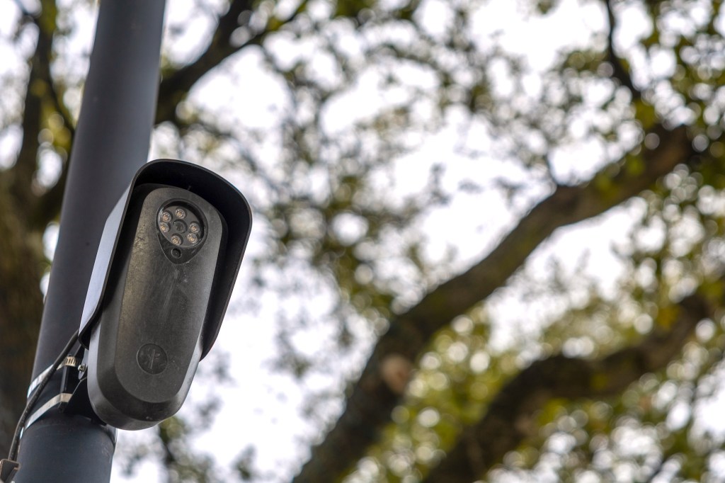
A Flock surveillance camera in Houston, Texas, US, on Wednesday, Feb. 4, 2026. Flock counts more than 6,000 customers that are using its license plate readers, camera-equipped drones, gunshot detection devices and software, with customers in every state except Alaska. Photographer: Antranik Tavitian/Bloomberg via Getty Images

LAPD lets contract with surveillance giant Flock expire, citing ‘serious concerns’ over civil liberties and privacy

The Los Angeles Police Department (LAPD) is reportedly ending its deal with Flock Safety, a surveillance company that helps law enforcement track vehicles using thousands of its license plate cameras placed across the United States.

A senior LAPD official told news outlets, first reported by ABC7 and the Los Angeles Times, that the police department would allow its three-year contract with Flock to expire when it ends on Saturday. The department cited “serious concerns” around civil liberties and privacy. Flock’s cameras are operated by the Atlanta, Georgia-based company and not the LAPD.

“This contract is not being renewed because of serious concerns around civil liberties and civil rights issues, particularly around privacy and the data that is being collected from these cameras,” LAPD’s chief information officer Dean Gialamas was quoted as saying. “The LAPD had to make a difficult decision, in this case discontinuing using Flock services until we can get those data, privacy, security and sharing concerns ironed out through a contractual relationship.”

A spokesperson for the LAPD did not respond to a request for comment from TechCrunch over the weekend, and it’s unclear if Flock’s cameras will continue recording in absence of an active contract. According to ABC7, the police department is seeking new language in its contract addressing privacy and data storage concerns.

As the third-largest police department in the U.S., the LAPD is one of Flock’s largest government customers to date. Several major U.S. cities have also stopped working with Flock, including Mountain View, California and South Portland, Maine, citing privacy worries and concerns that federal immigration officials used the cameras to track people in violation of their local laws governing their sanctuary city policies.

The contract expiry caught the surveillance company by “surprise,” said Flock spokesperson Holly Beilin in an email to TechCrunch. Flock said it was confident that the company could “clear up the current misconceptions” that led to the contract’s end. Flock would not say which specific misconceptions it was referring to.

Flock has a network of at least 80,000 cameras around the U.S. that scan license plates and allow police and federal agencies to track vehicles. 

The company has faced heavy backlash from local communities that have approved and then reneged on their deals with Flock over concerns with privacy and surveillance. Some locals have taken matters into their own hands by dismantling Flock cameras and covering them with trash bags, even as some communities found that Flock reinstalled cameras without permission from local authorities.

Researchers have identified an uptick in documented cases of motorists being pulled over, detained, and held at gunpoint by police, or jailed, due to false positives and errors with license plate readers. Last week, a journalist with car reviews and news website The Drive detailed how he was tracked for days and later boxed-in by police after a Flock camera mistakenly flagged the license plate of the on-loan review unit he was driving as stolen.

Flock has also faced scrutiny following several security lapses that have exposed cameras and data, which in one case allowed independent news outlet 404 Media to watch themselves live on publicly exposed Flock cameras. Lawmakers have also urged federal consumer authorities to investigate Flock for failing to implement measures that would prevent hackers and spies from gaining access to its security cameras, warning that many of the police user logins are not protected with multi-factor authentication.

404 Media also reported that the U.S. Drug Enforcement Administration used a local police officer’s password without their knowledge to search for a suspect accused of an immigration violation.

Do you know about security or privacy issues with Flock Safety, or issues with Flock cameras in your community? We would love to hear from you. From a non-work device, you can securely contact Zack Whittaker on the Signal messaging app with the username zackwhittaker.1337.

The Daily Front Page 10 of 26
Monday, July 13, 2026 The Daily Front No. 5 — Farewell to Sam Neill
article

Sam Neill has died

by j4mie·▲ 468 points·114 comments·theguardian.com ↗
Sam Neill, the versatile New Zealand actor whose career spanned Oscar winners and blockbusters such as The Piano and Jurassic Park, has died aged 78.

Actor Sam Neill smiling with arms crossed in a red plaid jacket in front of a wooden fence

Sam Neill has died aged 78. The actor is pictured at his home and vineyard, Two Paddocks, in Alexandra, Central Otago, New Zealand, in 2022. Photograph: Fiona Goodall/The Guardian

Sam Neill, star of Jurassic Park films, Peaky Blinders and The Piano, dies aged 78

New Zealand actor built career as dashing romantic leads and charismatic villains across film and television

Sam Neill, the versatile New Zealand actor whose career spanned Oscar winners and blockbusters such as The Piano and Jurassic Park, has died aged 78.

The actor’s death was announced on Monday in a statement shared on his Instagram account. No cause of death was given, but Neill had only recently revealed he was cancer-free after being diagnosed with stage three angioimmunoblastic T-cell lymphoma, a type of blood cancer, in 2022.

“It is with immense sadness that the whānau of Sam Neill share the news of his passing on Monday 13th July, in Sydney Australia. Sam was surrounded by family and passed with the dignity that has characterised his whole life.

“The loss was sudden and unexpected but blessed by the fact that Sam remained cancer free. They would like to express their deepest gratitude to the staff at St Vincent’s Private hospital for their incredible care.

“More details will be shared later, but for now, on behalf of the family, we ask that you respect their privacy as they navigate this immeasurable loss.”

Neill’s peers, friends and admirers paid tribute to him on Monday as news of his death spread.

Neill was born Nigel John Dermot Neill in 1947 in Omagh, Northern Ireland to an English mother, and a New Zealander father who was serving in the British army. The Neills moved to New Zealand in 1954. He took the name Sam when he was 12 because there were several Nigels at his school, and: “I found I moved more easily in the world as a Sam. Nigel is an awkward fit in most circumstances. Imagine being a movie actor called Nigel Neill.”

Neill attended school and university in Christchurch, but didn’t settle on acting until after he failed a “catastrophic” year of studying law. He began appearing in Canterbury University productions, and moved to Wellington to join the Downstage Theatre as a professional actor, where he was paid $35 a week and any leftover food from the kitchen from meals served to the audience before the show.

Sam Neill (centre) in a scene from the movie Jurassic Park

Sam Neill (centre) in Jurassic Park. Photograph: Album/Alamy

After some small roles on local television, his breakout role was in the 1977 film Sleeping Dogs, the first New Zealand film to open in the US. Soon after that he landed a leading role in My Brilliant Career (1979); played the son of the devil in Omen III (1981); appeared in Andrzej Żuławski‘s cult film Possession (1981); in the 1988 biopic Evil Angels (also known as A Cry in the Dark), as Lindy Chamberlain’s husband, Michael, opposite Meryl Streep; and in The Hunt for Red October (1990). His role in Ivanhoe (1982) made Neill a big name in Sweden, where the film has aired on TV every New Year’s Day for 40 years.

Neill came to widespread international attention in 1993 with two performances: as New Zealand settler Alisdair Stewart in Jane Campion’s Oscar-winner The Piano; and as Dr Alan Grant in Steven Spielberg’s Jurassic Park, a role originally offered to Harrison Ford. Neill played Alan Grant again in sequels Jurassic Park III and Jurassic World Dominion.

Sam Neill and Judy Davis in My Brilliant Career

Sam Neill and Judy Davis in My Brilliant Career (1979), directed by Gillian Armstrong. Photograph: David Kynoch/Margaret Fink/NFSAA

Neill shaped a career playing memorable romantic leads and charismatic villains. He had more than 150 credits over five decades, including Dead Calm, The Jungle Book, In the Mouth of Madness, Event Horizon, Bicentennial Man, The Dish and Peter Rabbit. He was one of the leading candidates to succeed Roger Moore as James Bond and did a screen-test in 1986, but lost out to Timothy Dalton.

In 2016 he starred in Taika Waititi’s breakout hit Hunt for the Wilderpeople, which led to small cameos in Waititi’s Thor: Ragnarok and Thor: Love and Thunder.

Neill also worked in television, playing the corrupt Maj Chester Campbell in Peaky Blinders, The Twelve, The Tudors, and episodes of The Simpsons and Rick and Morty. He was nominated for a Golden Globe for his portrayal of spy Sidney Reilly in the 1983 miniseries Reilly, Ace of Spies.

Neill lived on a farm and winery called Two Paddocks, in the Central Otago wine region. He described it as “a ridiculously time- and money-consuming business. I would not do it if it was not so satisfying and fun, and it gets me pissed once in a while.” He named his farm animals after his colleagues, including Laura Dern (chicken), Kylie Minogue (duck) and Helena Bonham Carter (cow).

In 2023, Neill revealed in his memoir, Did I Ever Tell You This? that he had been undergoing chemotherapy for a year after being diagnosed with stage three angioimmunoblastic T-cell lymphoma, a type of blood cancer. By the time his book was published his cancer was in remission, but he underwent monthly chemotherapy for the rest of his life, having signed a contract with the drug company that if he was still alive after four months, the treatment would be free.

“I’m not afraid to die,” he told the Guardian in 2023, “but it would annoy me. Because I’d really like another decade or two, you know? We’ve built all these lovely terraces, we’ve got these olive trees and cypresses, and I want to be around to see it all mature. And I’ve got my lovely little grandchildren. I want to see them get big. But as for the dying? I couldn’t care less.”

Sam Neill in Reilly, Ace of Spies

Sam Neill in Reilly, Ace of Spies. Photograph: Rex Features

He said he “dreaded” any prospect of retirement. “Some of it is to do with coming from a little place, the most obscure place in the world, as far from anything as you could get, and being asked to do something with an international dimension. How immensely seductive is that?”

Neill was appointed an Officer of the Order of the British empire in 1991 for his services to acting and a Distinguished Companion of the New Zealand Order of Merit (DCNZM) in 2007. Years later, after a change to New Zealand’s honours system allowed recipients to convert the DCNZM into a knighthood, Neill accepted a knighthood and gained the title sir in 2022.

Neill jokingly described his family life as “somewhat haphazard” due to his career. He is survived by his four children and eight grandchildren. His children are Andrew, who was placed for adoption when Neill was in his early 20s but reunited with his father in 1994; Tim, his son with actor Lisa Harrow; Elena, his daughter with makeup artist Noriko Watanabe; and Maiko, Watanabe’s daughter from her first marriage, who Neill adopted.

The Daily Front Page 11 of 26
Monday, July 13, 2026 The Daily Front No. 5 — Sega’s Cinematic Trickery
article

The art and engineering of Sega CD Silpheed

by ibobev·▲ 254 points·55 comments·fabiensanglard.net ↗
While the 640 MiB storage was 320x a cartridge capacity, the access time and bandwidth were an eye-opener.

The art and engineering of Sega CD Silpheed

The 90's was a decade of considerable improvement in the world of video-game consoles[1]. Each new model brought advanced processing power and better graphics without compromise.

The mid-90s emergence of CD-ROM drives however was an oddity. While the 640 MiB storage was 320x a cartridge capacity[2], the access time (800ms[3]) and bandwidth (single-speed 150 KiB/s) were an eye-watering 4,000,000x and 35x slower.

The Mega-CD was Sega's idea to bring CD-ROM to its Genesis console. Nearly 200[4] titles were produced for the platform. A few great games like Sonic CD, Snatcher, Final Fight CD, and RPGs came out. But an endless series of titles relying heavily on Full Motion Video (FMV) gave Sega's add-on an infamous reputation (Night Trap, Prize Fighter, Slam City, Corpse Killer, Supreme Warrior, WireHead, and A/X-101).

And then, there is Silpheed. Armed with exquisite artistic taste and an engine capable of jaw-dropping animation, it made the press go wild[5][6]. Players pondered what was real-time 3D and what was pre-calculated[7]. It received praises which, to this day, persist[8][9].

For those still unimpressed, keep in mind these near-fullscreen cutscenes run on a 12.5MHz m68k CPU, use 16 colors, and consume 150 KiB/s. With 16-bit 16kHz music, the 15fps video stream was left with a mere 8 KiB per frame.

I spent the past two weeks reverse engineering the FMV format in my spare time. That was a departure from how I normally work since I did not write a single line of code. I will likely write something about my A.I framework (and opensource it) next month. But I can already tell this is an overall pleasant way to work.

The following is what I came up with. And if you want to see all of the cutscenes and gameplay background videos to get accustomed to the topic, here is a storyboard I created with the tools I designed (I can't really say I "wrote" them).

Sega-CD internals 101

        GENESIS               │                      MEGA-CD                   
                              │                                                
┌──────────────────────┐      │               ┌───────────┐        ┌──────────┐
│ MC68000 7.67 MHz     │      │               │  WORD RAM │        │  MC68000 │
│                      │  ┌───┴──────┐        │   256 KB  │        │          │
│ 64 KB RAM            ◄──┤Expansion ├────────►───────────┤        │ 12.5 MHz │
│                      │  │   Port   │        │PROGRAM RAM│        │          │
│ 8 KB Audio RAM (Z80) │  └───┬──────┘        │  512 KB   │        │          │
└──────────┬───────────┘      │               └─────┬─────┘        └─────┬────┘
           │                  │                     └──────────────┬─────┘     
     ┌─────┴──────────┐       │                                    │           
     │                │       │                 ┌───────┐     ┌────┴────┐      
┌────▼──────┐   ┌─────▼─────┐ │                 │ Ricoh │     │  ASIC   │      
│ VDP       │   │   Z-80    │ │                 │  PCM  ├─────┤  GFX    │      
│ ┌───────┐ │   │   YM2612  │ │                 └───┬───┘     └────┬────┘      
│ │64KVRM │ │   │  SN76489  │ │                     │              │           
│ └───────┘ │   │           │ │                     │              │           
└─────┬─────┘   └──────┬────┘ │                     │      ┌───────┴──────┐    
      │                │      │                     │      │    CD-ROM    │    
      │                │   ┌──┴──────┐         ┌────▼────┐ │     DRIVE    │    
      │                └───┤RCA Cable├─────────►  MIXER  ◄─┤              │    
      │                    └──┬──────┘         └────┬────┘ └──────────────┘    
      │                       │                     │                          
 ┌────▼────┐                  │                     │                          
 │   TV    ◄──────────────────┼─────────────────────┘                          
 └─────────┘                  │                                                 

Adding a Mega-CD turns the machine into two systems running in parallel. The Mega-CD side has PCM and CD playback, connected directly to the mixer[10]. There is an ASIC with graphics acceleration (rot/scal/misc) to rival games like Mario Kart. The two systems communicate via shared memory (the expansion port) and analogic audio mixing.

Understanding how this thing works made me respect Mega-CD developers even more than before. This looks like a nightmare to deal with, especially synchronization.

The architecture of Silpheed

A Mega-CD system still renders to the TV with three layers. Two of them are made of tiles and called backgrounds (A and B) while one is the foreground containing sprites.

The Sub-CPU m68k writes the tiles and tilemap for background B. Meanwhile the main CPU takes care of "drawing" background A containing the HUD and the foreground sprite layer.

The Sub-CPU uses a double-buffer system where it renders to the Word RAM in L1 mode. While one buffer is fed to the VDP by the main CPU, it renders the next frame into the other buffer.

On the audio side, non-interactive cutscenes rely only on the Ricoh from the Mega-CD to generate PCM quality music. During interactive sequences, the Ricoh is sporadically used for PCM audio samples while the music is done via the YM2612.

Background A

Background B

Foreground (Sprites)

The original Genesis (Model 1) audio path is incredibly convoluted. The output of the Genesis, its front jack port, must physically be connected to the RCA input in the back of the Sega-CD via a "mixing cable". The Sega-CD then mixes the line-in signal with its own CD-DA + PCM signal. The result is sent direclty to the TV via another RCA cable!

Good design decisions

Most FMV games looked bad because developers followed a top-down approach trying to cram a real movie into a tiny CD-ROM using a weak CPU. To do so, they had to use a minuscule window, compression artifacts, and dithering that made you cry.

For Silpheed, Game Arts took the opposite approach. They started from the bottom, engineering upward from the constraints of the system. They made excellent trade-off decisions with flat shaded polygons, 16 colors total, no gouraud, and minimal dithering.

This approach would have never succeeded without the talented artists of Game Arts who were able to go the distance with these choices (especially the limited number of colors).

PC-CDROM games were a different story. Thanks to better CPUs (DX4-100) they were able to use much better codecs. Some well-funded games, like Command & Conquer, Crusader: No Remorse, or Wing Commander III (4 CDs!) used FMV to tremendously improve the storytelling.

The bandwidth problem

At its core the problem of FMV is a problem of bandwidth. Data needs to be extracted from the CD-ROM, decompressed by a processor into an image, and that image must be fed to the video screen to find its way to the TV. The Mega-CD is ill-equipped in all three stages.

The tilemap problem

At first sight, there is another problem. Without a framebuffer, rendering must follow a cumbersome process where 768 tiles of dimensions 8x8 are drawn into. The tiles are then laid out on the screen, 32x28 via a tilemap (traditionally called "nametable" in Genesis parlance). The result forms a 256x224 image.

Three easy ways to reduce bandwidth

The easiest way to reduce bandwidth is to reduce the size of the video. Silpheed also uses this trick but just a little bit with the top and bottom tile line set to black (that is 16 lines total). It almost looks like an artistic choice since it results in a cinematic aspect ratio!

The second way to reduce bandwidth is to reduce the framerate. Silpheed uses mostly 15fps with some complex scenes going as low as 7.5fps.

Finally, the third way to reduce bandwidth is compression. For this, cutscenes and background video are handled differently.

Video Compression

Silpheed does not use delta-compression. Every frame in a video is self-sufficient. Every single frame contains all the tiles it needs and the tilemap to place the tiles on the screen.

Written like that it looks like there is no compression at all. But that is where the cumbersome tilemap system becomes a tremendous source of optimizations. Let's take the example of frame 44 in the "Game starts" cutscene.

If we add an 8x8 pixel grid, we can see the image has interesting properties. For example, a lot of tiles are the same plain color.

Silpheed's video format extensively exploits this. The encoder only issues one of each of the 15 plain color tiles in a frame and then references it over and over again in the tilemap. For this frame, out of 896 tiles, 456 reference the same 15 single color tiles. That is a bandwidth reduction of 50% right there.

On the right, we have all the leftover tiles made of more than one color. For these as well, Silpheed has a trick up its sleeves.

Leveraging Mega-CD ASIC for decompression

With 456 tiles taken care of, 440 remain (see the image below). Some of these tiles also have an interesting property. They are made of only two colors.

The Mega-CD ASIC features advanced graphics capabilities. The most famous ones are rotation and scaling (to be able to rival games like Mario Kart on Super Nintendo). A much less notorious feature is named "Font bit"[11]. As its name indicates, the intent was to allow fast 2-color kanji/text rendition. With three bytes, the font registers generate 16 nibbles (8 bytes) which is two full rows of an 8x8 tile. Here is how it works.

  1. Write two 4-bit palette indices to the source color register ($FF804D).

    • Color A = pixels generated when a bit is 0
    • Color B = pixels generated when a bit is 1
  2. Write a 16-bit bitmap pattern to $FF804E.

    • Each bit represents one pixel.
    • The 16 bits are interpreted as two rows of 8 pixels.
    • A 0 bit selects Color A.
    • A 1 bit selects Color B.
  3. The ASIC expands the 1-bit pattern into 4-bit pixel data.

  4. Read the generated tile data back from $FF8050-$FF8056.

With three bytes, the font registers generate 16 nibbles (8 bytes). That is 37% bandwidth saved on the 50% remaining from the first optimization. Not to mention the CPU time saved not having to mask bits to write nibbles.

Above, on the left, are 234 tiles, made of two colors. These were generated via the ASIC "font registers". On the right is what remains, 206 raw tiles that are actually stored as 8x8 "raw" nibbles in the frame.

Tilemap compression

Each frame has a tilemap and this also is compressed. Normally the 768 tile locations would have taken 768x 10bit = 960 bytes. The compression scheme leverages another property of the image, namely that tile indices in the tilemap increase linearly (as shown in the 8x2 tilemap below).

0 1 2 3 4 5 6 7
8 9 A B C D E F

The tilemap is stored as a 768-bit bitmap (96 bytes) where 0 means "auto-increment" and 1 means read an immediate value. In practice, the trick reduced the space requirement by nearly 30% (96 + 556-byte payload = 652 bytes).

Fractal level

If you refer to the storyboard, you will see that two levels (Stage 1 and Stage 10) include complex textures (which in interviews were called "fractals" by developers). These sequences were very hard to compress. So much so that all tiles use raw format without any trick. The only way to make it work was to drop the framerate to 7.5fps.

Palette trick

If you take a look at the actual gameplay you will have noticed that the laser and explosions do not use a plain color. They are in fact multi-colored. This effect is achieved by reserving four colors at the end of the palette and shifting them each frame via the main m68k.

This also means artists had to design gameplay sequences using only twelve colors (cutscenes used the full 16 colors since there was no laser effect in them)!

References

^[ 1]Consoles of the 90s ^[ 2]Wikipedia: Mega-CD ^[ 3]VG Museum, Sega-CD ^[ 4]List of Mega-CD games ^[ 5]Silpheed/Reception ^[ 6]Silpheed.comp: Magazine articles ^[ 7]Silpheed backgrounds and cutscenes ^[ 8]Why DOES Silpheed's FMV look so good? ^[ 9]Sega CD Silpheed Was Largely Just Spectacle, But That’s Okay ^[10]Mega-CD V1 manual ^[11]MEGA-CD SOFTWARE DEVELOPMENT MANUAL

The Daily Front Page 12 of 26
Monday, July 13, 2026 The Daily Front No. 5 — Linux Finds a 32X
article

Linux on the Sega 32X. Who needs hardware synchronization primitives anyway?

by cakehonolulu·▲ 145 points·32 comments·cakehonolulu.github.io ↗
Who needs hardware synchronization primitives anyway?

Preface

I couldn't start this entry in any other way possible but by thanking everyone who enjoyed the Linux on Jaguar post.

Also special props to the linuxmd project again.

It was a very fun experience and we've even made it into a few news outlets:

Hackaday Hackaday

or

Tom's Hardware Tom's Hardware

I also posted it on Hacker News and it recieved some good interest (And nice questions!).

So, yes; thanks everyone again!

Why is this (Linux) trend continuing?

I have an easy answer to this question, it's mainly to improve my board bringup skills.

I've been working professionally on the Firmware/Operating Systems/Embedded area for well over 2 years now (Professionally-speaking) and one of the usual suspects you see when trying to land a new job is "the ability to handle board bringups from the ground up".

I know it doesn't sound too fascinating but for me, other than job hunting (Which is not my bread and butter anyway), bringing up a piece of silicon and having it run something you made/helped making is super fun. You get to experiment with many of the different layers that make the result up: Emulators, Technical documentation, Experimentation, Investigation... you know; the usual engineering stuff.

Not that reading early-90s scanned datasheets is my passion (There's some documents that are plain images embedded onto a PDF) but there's something to it that makes me come back every time.

I actually started doing this in '13/'14. I was 12/13 at that time and I vividly recall my parents buying me my first phone. It was a MediaTek-based 6589 quad-core processor with a gig of RAM. Powerful stuff eh!

At that time (Not much soon after), Google released Android 5.0 Lollipop; but the vendor of the phone decided that it would not update it to that version. And I was really sad... so I had to get my hands dirty.

I'll sum up the story a bit because it's a bit large, but the gist of it is that I asked the company to comply with GPL and release the Linux kernel source code for the phone; for which they opposed, but as a community we got together and they released it (Along some other phone's trees).

Picture me surprised when the source code was half-assed and the board configuration didn't boot on the phone. Fortunately at that time, I found a leak of the full-source of MediaTek ALPS targetting a variation of the 6589 that seemed promising enough (Had the full Little-Kernel bootloader, Baseband, Preloader, Linux kernel and AOSP) for me to check.

I spent a few months trying to reverse-engineer parts of the zImage that was bundled on the stock boot image provided by the phone vendor to fill parts of the MediaTek code (Mostly related to lcm, battery, chipset quirks and whatnot) and after some good amount of digging and experimenting (And good chats with the cool people over at xda-developers) I had Android 5.0 running on my phone; mind you, it wasn't perfect. No Bluetooth, no HWComposer (Hardware acceleration), no Media engines... but seeing the pure, unadultered new Material Design on my phone blew my mind.

Android 5.0 Lollipop Android 5.0 Lollipop

I should probably try to make a separate post of this story... someday.

The mighty Sega 32X

Released in November 1994 in America/Europe (December 1994 on Japan); the Sega 32X was an add-on that promised to be an intermediate step between the 16-bit era Genesis and the soon-to-be 32-bit Sega Saturn. I'm not a good writer so the story that led up to that particular moment (For SEGA, that is) is a bit tumultuous (SEGA Japan vs SEGA of America) so I'll leave it as a task for the reader.

Anyhow, prior to the 32X, SEGA launched a CD add-on; the Sega CD (Or Mega CD, if you are european/japanese). It plugged into the expansion slot of the Genesis and it enabled CD-quality audio streaming (And well, game/game asset streaming). It was a machine on it's own (It had a higher clocked 68000 in comparison with the Genesis). There were 2 separate models, the first "generation", which was front-loading...:

Sega CD 1 Sega [Mega]CD Model 1 with Mega Drive/Genesis Model 1

...and the second, top-loading one:

Sega CD 2 Sega [Mega]CD Model 2 with Mega Drive/Genesis Model 2

But this post is about the 32X... so here it is:

Sega 32X Sega 32X

The actual addon was plugged into the cartridge slot of the Genesis (It had a separate power brick and video output, later of which was "combined" on-top of the Genesis video out timing/video/color channel signals).

Sega 32X & Genesis Model 2 Sega 32X & Genesis Model 2

If you've ever had the pleasure of building the Tower of Power, you'll know that having 3 separate power bricks, plus the cables to get stereo output out of the 32X, the "patch" cables and the many missing tidbits I'm probably forgetting now, wasn't anything short of fancy.

But what did all of that power?

32X Hardware specifications

Admittedly, the addon is far more powerful than the base console:

Component(s)Sega Genesis/Mega DriveSega 32X Main CPU1 x Motorola 68000 @ 7.6 MHz2 x Hitachi SuperH SH2s (SH7604) @ 23 MHz Bits16-bits32-bits Max. on-screen colors6432768 System RAM64KB+256KB SDRAM (Along Genesis's 64K) Video RAM64KB256KB (Double-buffered) GraphicsSprite-basedSoftware-rendered 3D (Flat shaded, goraud shaded, simple texture-mapped polygons)

As you can see, quite the difference. I've not even listed all the differences, but the main ones I can think are those.

Unfortunately for SEGA, the launch happened almost at the same time as Sony's PlayStation 1; which was primed to overcome the gaming industry with a much simpler architecture. It also didn't help in any way that the SEGA Saturn was close to launch date too (So consumers were puzzled as to which one to get). All in true SEGA fashion!

Anyway, if we got Linux running on the Jaguar, we should be able to do similarly for the 32X; right?

jmp _linux, the rendezvouz

Getting Linux to run on the SH2s (Running as in, having it print anything meaningful over UART) required some brainstorm.

We'd need to set up 3 different CPUs, the 2 x SH2s and the 68000. Fortunately there's readily-available examples for that on Github so I picked what seemed the most popular 32X Hello World example: Chilly Willy's Sega MD/CD/32X devkit.

The basic example sets up a communication channel between the 32X(s) and the 68000 (So you can ask the 68000 do some stuff the 32X can't) through specific memory-mapped IO addresses; prepares the SH2s (Sets up the caches, uploads the SH2 code from the cart directly off of 68000 machine code...) and makes the primary SH2 jump to it; whilst the secondary gets parked.

What I did was, expand this so that I could have a simple state machine that pushed characters to the UART on the Genesis (Since the 32X doesn't have direct access to it); but there was a problem...

256K + 64K

The biggest hurdle when porting Linux to a new (And newer-ish, in terms of when it launched) platform is mostly about doing the wiring to get it up and running; that's usually the case if you have the memory to even load it. This is not the case for us...

Fortunately, there's FPGA-based flash carts for the console (Enables you to run games for both the base model and the 32X; and there's even specialized "cores" that provide Sega CD support if you don't have the add-on!). One of those (series) of carts comes from Krikkz.

He basically did what flashcarts do but went the extra mile for pretty much everything, it's not just about running games!

There's a special bit of those carts that we're interested on:

Extended SSFv2 Mapper

Older cartridge-based systems often had this notion about "mappers".

Mappers are basically ICs that sat on the cartridge which enhanced the capabilities of what the console can handle in terms of memory.

They could also offer other features not related to memory, an example is Sega's Virtua Processor (SVP), which had a Samsung-engineered DSP to do heavy math computation (To enable Virtua Racer to display all it's 3D polygon glory on a base Genesis); or Nintendo's SuperFX chip; which provided similar capabilities to the SVP and was made by the creators of Days of Thunder or Birds of Prey: Argonaut Games.

Usually mappers were used to enable more ROM space for larger/more detailed games in a bank-switch fashion. You'd write to a certain memory address/do a specific set of accesses and the IC would internally remap parts of the "extended" ROM to the memory window the console can directly address. Kinda like MS-DOS's HIMEM.SYS in spirit if you think about it.

So Krikkz basically did us all the work here, turns out we can have ROM as RAM (ROM which can be made "writeable" by arranging certain configuration bits). This gets us 4 MBs of RAM.

I had to basically extend the SDK example to do the ROM->RAM mappings but had to leave a bit of space for the Linux + initramfs binary to live on (The actual ROM within the cart memory window, basically). I ended up finding a sweet spot of 540~KBs of ROM and rest of RAM. The Linux loader basically copies the binary on the memory location it was linked at and jumps to it.

Compiling and running Linux

So, I made a sh2eb-elf cross-compiler and got to compile Linux... but the compilation failed rather soon.

Out of all the issues I've had with toolchains, this one was probably the funniest.

For some reason GCC was having an ICE (Internal compiler error) when compiling kernel/nstree.c. I was able to find a workaround (Didn't have the time at that moment to file a bug report) fortunately.

After all this work (And writing a small earlycon driver to get some UART output carried from the 32X to the Genesis) I had the very first Linux messages.

There was a separate issue, at some point Linux seemed to stop the boot process and was hanging indefinitely.

I then discovered another set of issues, this time regarding: ashlsi3, ashrsi3 & lshrsi3. I'm not really sure how those are written (Do they get copied/inspired from their libgcc-counterpart or something similar?) but comparing what the cross-compiler did for those and what Linux did, it was obvious that we were clobbering a register we should not be clobbering. I found this because I started noticing that some pr_info(s) and pr_notice(s) were getting it's stack corrupted (And never returned to the caller) and was able to trace it here.

I then made an additional (Similar) fix for arch/sh/lib/checksum.S just to be on the safe side of things; where I basically gated shrd because it doesn't exist on the SH2s contained within the 32X (And if used... Illegal Opcode).

This basically got us through the entire boot process right before the clock calibration; for which I decided to make a simple driver for the SH2(s) FRT (Free running timer); this also got us further and we were at the verge of launching the init process.

Fortunately, this time around I was able to leverage ELF FDPIC support (Which made my life easier in comparison with Jaguar's FLAT binary support) to build my rootfs. I was also blessed by musl-cross-make; which landed me a sh2eb-linux-muslfdpic- toolchain I could use (I must say I battled hard with crosstool-ng, buildroot and a few others but didn't succeed).

So with this, everything was booting.

Case... closed...?

SMP

Yeah, I couldn't help myself.

It turns out that you need some hardware primitives to enable inter-CPU synchronization... which the SH2s on the 32X don't have¹.

¹: TAS.B opcode seems to be used on projects like D32XR even after the developer manuals asked not to do so due to the adapter bus not having the locked read-modify-write cycle mechanism.

We also don't have cache coherency so another problem to add to our bag.

But I thought, hey, both SH2s are equal features-wise; we sure can come up with something... right?

It turns out that sparc32 has precisely some code to aid in that.

We can basically leverage Peterson's algorithm to implement the required primitives entirely in software. Mind you that this isn't performant but it does work.

I basically had to do the bringup for all the primitives that needed care (cmpxchg, for instance) with the ideas that Peterson described.

I also needed to wire the 68000's code (Which for now was only handling UART stuff) to aid on delivering IPIs to both SH2s (I extended the commands the 68000 can receive so that it could correctly do it's thing) plus setting up the shared memory region to aid on the syncronization tasks. Think of the 68000 as being a bus arbiter/extra interrupt router at this point.

From the SH2s I just send an "IPI" command which the 68000 parses and decides which interrupt line to assert based on a bit of the data word (0 primary, 1 secondary).

Then there's the cache-coherency issue, which I solved by not using cached mappings (And well, cache is disabled, regardless) to place Peterson's flag and turn variables (You know, to avoid SH2s spinning on stale cache values for flag; for instance).

There was another issue I faced, how do I identify which CPU is which (So Linux can properly manage and issue hard_smp_processor_id()): Well, considering I was doing softfloat regardless; I just made the CPUID_REG point to the SH2-private hardware divider register (DVSR) which had no other use so it effectively became my what cpu am i register. That register is written by the Linux loader at boot for both the primary and secondary SH2s.

Performance is abysmal, bus contention is bonkers; but it does work, and that's fine by me.

smp: Bringing up secondary CPUs ...
MARS SMP: released secondary SH2 to 22082000
smp: Brought up 1 node, 2 CPUs

I must admit that it wasn't as easy as that, it really involved lots of tinkering and (Mostly) trial-and-error (I also spent 2 nights chasing why both CPUs would get woken but soon after they'd idle, turns out I needed a fix on default_idle() that was making the scheduler bug out and not correctly continue execution).

But it was well worth it.

I just then basically made a simple console display driver (So you know, you could see it in action in your actual screen)...

Linux on 32X

Voilà

Needless to say that all of this required lots of fine-tuning (I was also OOM-ing constantly and needed to put both Linux and Busybox through a good diet) but it was again, a very rewarding experience.

Misc. config. files if anyone wants to try

Linux tree (mars_defconfig)

Busybox config

Init script

The Daily Front Page 13 of 26
Monday, July 13, 2026 The Daily Front No. 5 — First Board, First Sparks
article

Designing and assembling my first PCB

by tadasv·▲ 162 points·93 comments·vilkeliskis.com ↗
I had this sudden itch and I wanted to play around with hardware.

The beginning

About a couple months ago I purchased an Arduino Nano ESP32 dev board. I had this sudden itch and I wanted to play around with hardware. I don't really have much experience in this space, besides working on firmware for an IoT company over a decade ago, but I've written tons of software over the years. I was very surprised how quickly I was able to get the built-in LEDs to blink with Arduino IDE and some help from LLMs. After that I moved on to figure out how to build and flash firmware directly from the command line without having to deal with all these custom abstractions. I like operating from CLI. That was also somewhat easy and gave me confidence that I can go back to my normal tools (nvim) for working with code.

The devboard itself does not have much going on. Next was getting some peripherals so I ordered a small LCD and BME280 temperature/humidity sensor breakout boards. Both of these I was able to wire up to the ESP32 chip and get them to talk over the I2C protocol.

Playing around with Arduino Nano and random things attached to it via breadboard

Figure 1: Playing around with Arduino Nano and random things attached to it via breadboard.

Naturally, we cannot continue assembling pre-existing modules for a variety of reasons. I think they are great for prototyping, but I like getting out of the prototyping phase as soon as possible and getting into a more "release" or "production" workflow. I was thinking maybe I should recreate the Arduino board with all these components hardwired so I can ditch the breadboard. That sounded great, but it felt a little bit ambitious. There's lots of components and it would make it hard for me to test everything. Instead, I decided to create the BME280 sensor module. This would let me get a feel for what it takes to design something starting with schematics and ending up with a custom PCB. In the picture above you can see the small brown board that I got from Amazon, that's a BME280 sensor board which only has a handful of components. If everything goes as planned I should be able to swap-in my custom board and everything should continue working as before. That was the plan.

Schematic and PCB design

There seem to be several tools available for schematic/pcb design. I needed something that's free and runs on Mac OS. Some people praise EasyEDA, others like KiCad. I didn't do much research on this topic, it seemed like either of them would fit the bill, but I picked KiCad since it's free GPL licensed software.

All sensors, chips and components come with what's called a datasheet. A datasheet is a technical document made available by the manufacturer describing how the component functions, at what temperatures it can operate, reflow (soldering) temperature curves, size and exact dimensions, example wiring and many other things depending on the component.

For my sensor module, I needed to wire the BME280 for an I2C interface to make it plug-and-play. The module that I purchased from Amazon actually supports both I2C and SPI. So what I'm doing is not an exact copy, but actually a more narrow implementation. The BME280 datasheet has pin-out and connection diagrams starting on page 38. It actually provides examples for both SPI and I2C connections. I took the provided I2C connection diagram and transferred it to KiCad.

Schematic design of my sensor module

Figure 2: Schematic design of my sensor module.

I wouldn't call KiCad the most intuitive application for first-time users. However, I was able to draw up the exact schematic as was shown on the datasheet.

To transfer a schematic to a PCB you need to select what's called a footprint for each component. For example, there's only one type of BME280 sensor and it really has only one shape/size (aka footprint) available. That's not the case for other types of general use components such as resistors or capacitors. What footprints you pick will dictate the size of your board, how easy it is to assemble and most likely many other factors that I'm not aware of (such as heat dispersion).

Through my research I discovered that most commonly you're going to encounter SMD and THT components. THT or through-hole components are more old-school looking tech (though it's not old), generally larger in size and they get installed by pushing component legs through the holes in the PCB and soldering the legs to the board after. This can be done in most cases with a regular soldering iron.

SMD stands for surface mounted devices and are what you'd find in almost all modern electronic devices. They are much smaller in size, and as the size gets smaller, they will require more specialized equipment for installation. When I started looking at the footprint library in KiCad I got very confused because it wasn't immediately clear to me whether I needed to find a footprint for the exact component brand that I was planning to use or not. Lots of general SMD components have standardized footprints, I discovered. They follow standard codes like 1206, 0805, 0603, etc which translate to dimensions 0.12" by 0.06" or (3.2mm x 1.55mm) for a 1206 component. I went with the 0805 size as this seemed to be suitable for hand soldering, though it's pushing the limits.

After you assign a footprint for each component you can then import them into the PCB editor and layout your PCB.

My sensor module in KiCad PCB editor

Figure 3: My sensor module in KiCad PCB editor.

Module 3D preview

Figure 4: Module 3D preview.

The layout process did not seem too complicated, however, you need to be aware of how you are routing the connections, or they could otherwise prevent other ones from getting to their destination. I was able to layout everything on the front layer of the board. The only thing I did special (maybe that is not so special) was ground filling empty space on the front and back and then connecting front to back using via. This seems to be a common pattern used in the PCB design. Otherwise, it can get really tricky to route the connections without blocking other ones, even for a small simple board like the one I'm making here.

Sourcing components and ordering PCB

The component search was somewhat interesting too. I purchased my components from DigiKey. Although, it's probably best to have accounts with several electronics shops, just in case there's a limited inventory. I was able to find all components on DigiKey except for the BME280 sensor itself. The BME280 sensor was out of stock on several sites and it looked like it would take several months to get the backorder processed. I skipped the BME280 and decided to rip it off from the Amazon module I purchased earlier. The resistors and capacitors were somewhat easy to find, I just had to be careful picking the correct footprint and configuration (resistance etc).

KiCad also lets you generate a bill of materials (BOM). It's just a list of components and their configuration and where they need to be placed. The PCB manufacturers can sometimes perform the assembly for you if you provide them with the BOM. I did not do that, I wanted to hand assemble to get a feel for it.

BOM

Figure 5: BOM.

To order a PCB you need to export gerber and drill files. The gerber files define trace layout and the drill file is for the CNC machining. I exported both of these with default settings and packaged them into a zip file which I then provided to JLCPCB. From there you finish the order form. I did not make many changes and used defaults. JLCPCB is a Chinese company, order to door took about 2-3 weeks and cost me under $10 dollars. There are faster options, but they would break the bank on delivery costs.

My tools and assembly

As part of my current homelab, I only have two soldering tools plus a multimeter.

Hakko FX888DX-010BY

Hakko FX888DX-010BY soldering iron

Figure 6: Hakko FX888DX-010BY soldering iron.

I purchased this iron because it lets you control the temperature and it has pretty good reviews. It heats up really fast. I usually run my iron at 650F. However, temperature adjustment is critical so you know exactly what temperature you're getting so you don't damage the components.

Quick 861DW

Quick 861DW hot air station

Figure 7: Quick 861DW hot air station.

This device is called a hot air station, sometimes reflow or rework station. It is used heavily in electronics repair shops to replace components. You also can use it to solder SMD components. Once you go below 1206, using a soldering iron gets tricky. The way SMDs get soldered is by spreading solder paste over connections, placing the components on top and then microwaving the board using a hot plate or hot air gun to melt the solder. The hot air gun is the most versatile tool and it's good for smaller assembly.

I picked up a Quick 861DW because it's considered a pro entry-level device (according to LLMs at least). The most important part for a device like this is airflow control. I run this device on airflow setting 15 (which is very low volume) and 250C. SMDs are tiny and very light devices, anything that does not give you good air control will blow away the components.

The assembly

It took me about 15 minutes to assemble the board. That involved desoldering the BME280 sensor from the Amazon board, applying solder paste and laying out the components and soldering everything up. The only thing I struggled with was the sensor. The sensor is tiny and it has 8 connection pads underneath it so I wasn't sure if I would short any of the connections by accident because I couldn't see what was going on under the chip. I kept the area for the sensor clean and made sure there was flux on it and I left the rest to the surface tension gods.

My board vs board from Amazon

Figure 8: My board vs board from Amazon.

The results

I was giving this whole thing a 50/50 chance of working on the first try. I wasn't even sure if I routed everything correctly on the PCB. The "via" and grounding were a bit confusing. Then, soldering the sensor was slightly tricky and I wasn't sure if I shorted connections anywhere. However, to my surprise, the board I designed and assembled was plug-and-play on the first try!

My sensor board is working

Figure 9: My sensor board is working.

I did not have to modify the firmware, I did not have to put anything in between the board. It was literally a plug-and-play experience because I exposed the same I2C interface that I used originally.

This experience gave me confidence that I can produce custom and working PCBs. This, of course, was a very simple project, but it took me through the whole process end-to-end. It gave me a better understanding of the steps I may need to take for more complex designs. I was thinking maybe for the next one I should place the LCD, ESP32 and BME280 on a single board, hardwired. This one sounds a bit more complex. How do you flash the chip? How do you supply power? What is necessary and what is not? For example, the Arduino Nano dev board has lots of components on it. Are all of them needed? I have no idea. I will see what I'll do next, but I enjoyed this experience.

The Daily Front Page 14 of 26
Monday, July 13, 2026 The Daily Front No. 5 — E-Waste Horsepower
article

Benchmarking 15 “E-Waste” GPUs with Modern Workloads

by eso_logic·▲ 141 points·54 comments·esologic.com ↗
Decommissioned NVIDIA enterprise GPUs are one of the last remaining sources of idle VRAM.

Decommissioned NVIDIA enterprise GPUs are one of the last remaining sources of idle VRAM. K80 with 24GB of GDDR5 sells for $60, P100-16GB for around $75 and V100-16GB for under $200. Shortcomings and all, it’s important to understand if we can utilize these widely available cards in the modern era. This project to benchmark tesla GPUs has been in the works for almost a year and over the winter I was able to spend many kilowatt hours heating up my studio with GPUs.

https://esologic.com/wp-content/uploads/2026/07/22-tesla-benchmark-16-9-noaudio.mp4

Box of Tesla GPUs

A goal of all this benchmarking is to come up with a BOM for an inexpensive, 4U GPU node for my homelab. With the right cooler (if you’d like a beta unit of the cooler, join the email list!), these cards are happy to be installed much more densely than their consumer-oriented counterparts. One can easily fit three GPUs and a 10GB NIC into a standard ATX case, rack mount or otherwise.

Similar to GPU price, the cost of X99 Intel E5-* Xeon CPUs and their associated hardware are now so cheap they can’t be ignored. $40 gets you 56 threads @ 3.50 GHz boost using E5-2690. The going rate is $200 for the massive Supermicro X10DRG-Q with its two CPU sockets and 7 PCIe slots. Choosing the CPU and motherboard for a  GPU box is obviously important, but I wanted to have some hard numbers comparing the different schools of thought.

Don’t Be Afraid

Let’s note that all the hardware under examination here has been EOL’d. None of the GPUs are going to get CUDA compatibility updates or drivers anytime soon. Older gear is also going to be less power efficient, consuming much more energy per token. It is irresponsible to suggest these cards be used today.

… is the kind of finger wagging that has no place in homelabbing. The lack of software updates can be easily worked around by just using slightly older software. llama.cpp for example supports many CUDA architectures if you’re willing to build it from source. Using docker, I was able to get all of the software described below running on Kepler, an architecture released in 2014!

The power efficiency perspective is totally valid for high availability usecases. If you’re building something that is going to be used around the clock, you’ll quickly spend your savings on GPUs by paying for electricity. However this is also just not a usecase that is super relevant in the homelab. You’re not using LLMs or doing video processing? Turn off the box.

Content of the GPU Benchmarks

The benchmarking tool itself is published on github and I have already written a blog post about the development of the suite. Still though, here is a short description of the tests that appear in the resulting graphs.

Benchmark Category AI Description
ResNet50 Train B=64 Computer Vision Training Measures GPU performance when training a convolutional neural network for image classification.
ResNet50 Infer B=1 Computer Vision Inference Measures low-latency image classification inference on a single image.
ResNet50 Infer B=256 Computer Vision Inference Measures high-throughput batched image classification inference.
Blender GPU 3D Rendering Benchmarks production-style GPU path tracing for professional 3D rendering workloads.
Blender CPU CPU Rendering Provides a CPU rendering baseline using the same Blender scene.
CAT ViT Scores Vision Transformers Measures Vision Transformer inference throughput for image analysis and scoring.
CAT ViT Attention Vision Transformers Measures Vision Transformer attention map generation, a more computationally intensive analysis workload.
llama.cpp Qwen2.5 1.5B Prompt Large Language Models Measures prompt processing (prefill) performance for a small language model.
llama.cpp Qwen2.5 1.5B Gen Large Language Models Measures autoregressive text generation throughput for a small language model.
llama.cpp Llama 3 8B Prompt Large Language Models Measures prompt processing performance for a larger language model.
llama.cpp Llama 3 8B Gen Large Language Models Measures autoregressive text generation throughput for a larger language model.
llama.cpp Qwen1.5 MoE Prompt Large Language Models Measures prompt processing performance for a Mixture-of-Experts language model.
llama.cpp Qwen1.5 MoE Gen Large Language Models Measures text generation throughput for a Mixture-of-Experts language model.
F@H Single Scientific Computing Measures scientific compute performance using molecular dynamics simulations.
F@H Double Scientific Computing Measures scientific compute performance under a heavier molecular dynamics workload.
SHA-256 Cryptography Measures raw cryptographic hash computation throughput on the GPU.
Whisper Med FP16 Speech Recognition Measures transformer-based speech-to-text inference performance.
Storage→CPU→GPU (gdsio) AI Infrastructure Measures the throughput of loading data from storage into GPU memory, an important bottleneck for large AI models and datasets.

Theory of Operation

The goal of the utility is to be able to benchmark Tesla GPUs, “GPU Box” style servers. The theory of operation for the benchmarking suite is as follows.

Benchmarks are defined as dockerfiles and run as docker containers for compatibility and portability. The containers are run first on each type of GPU attached to the system. For example if there is a K80, an M10 and a P100 in the system, the container is run first with one of the two cores on the K80, then on one out of the four cores on the M10, and then once on the P100 because it only has one logical core. Then the container is re-run on all attached cores of all attached GPUs in parallel. Finally, if the test is multi-GPU native, a container is created with access to all cores of all GPUs and the test is run. This is an example result for a system with 3 P100’s running a ResNet50 training test:

{
    "name": "resnet50_train_batch_64",
    "benchmark_version": "0.2.0",
    "override_parameters": {},
    "larger_better": true,
    "multi_gpu_native": true,
    "verbose_unit": "Images Processed / Second",
    "unit": "i/s",
    "critical_result_key": "native_multi_gpu_result",
    "numerical_results": {
        "min_by_gpu_type": 208.20215154739634,
        "max_by_gpu_type": 208.20215154739634,
        "mean_by_gpu_type": 208.20215154739634,
        "theoretical_multi_gpu_mean": 208.2021515473963,
        "theoretical_multi_gpu_sum": 624.606454642189,
        "forced_multi_gpu_numerical_mean": 205.4402100738262,
        "forced_multi_gpu_sum": 616.3206302214786,
        "native_multi_gpu_result": 566.5793352441259
    }
}

The theoretical_multi_gpu_sum value is numerically calculated by taking the per GPU score summed over all the GPUs attached to the system. In our example, if the single K80 core scored 10, this value would be counted twice in theoretical_multi_gpu_sum. If the single M10 core scored 5, this value would be counted four times in theoretical_multi_gpu_sum. The next calculated value theoretical_multi_gpu_mean is computed by theoretical_multi_gpu_sum and dividing it by the number of GPUs attached to the system. The result forced_multi_gpu_sum is calculated by taking the sum of the results from the parallel run. Similar to the other mean value, forced_multi_gpu_numerical_mean is created by dividing forced_multi_gpu_sum by the number of GPUs. All of these different figures eventually be used to identify performance bottlenecks in GPU boxes or the tests themselves.

Currently, only the keys defined with critical_result_key are used in the visualizations. As of writing, these are all either native_multi_gpu_result or forced_multi_gpu_sum. Subplots titles marked with an asterisk are forced_multi_gpu_sum.

Hardware Under Test (Benchmarked Tesla GPUs)

GPUs: K80, M10, M40, M60, P40, P100, V100, T40

CPUs: E5-2687W 12-Core, E5-1680 8-Core

Motherboards: Asus X99-WS single socket, Supermicro X10DRG-Q dual socket

Results

Unless otherwise specified CPU and motherboard are the same within a set of results. The same RAM, chassis and power supply was used in every test. All GPUs were cooled with my cooler set to auto.

GPU Generation Comparison

For this first set of tests, we’ll be looking at results grouped by general usecase area across GPU generations. The expectation here is that in general performance should increase with release date, and the resulting bars left to right are ordered by the corresponding card’s release date.

There are a few surprises right off the bat here. The overall performance of Tesla V100-16GB is right up there with (the somewhat rare) T40 in all tests. V100 is significantly older and less expensive than T40. Generally too, there is a major increase in performance with Volta over the previous incremental gains achieved in previous generations.

If you read for any amount of time online, you’ll find people recommending P40 over P100 for LLM usage and these results hold that finding as well.

I was very impressed by M60’s Whisper performance. If you have a ton of audio transcription to do, M60 can be had for only $50.

GPU Scaling

This next set of tests examines how performance changes as more cards are added to the system. The expectation here is that generally test performance should increase with the number of cards added to the system but with diminishing returns as more communication overhead is added.

Interestingly, we see that LLM throughput stays the same as more GPUs are added. This points to a llama.cpp configuration issue on my part. PRs always appreciated if you know what is going on here.

For both K80 and P100, I’m really not seeing a ton of evidence of those diminishing returns except for CAT ViT Attention on P100. Other, more mature multi-GPU native tests (ResNet50 and SHA-256) increase linearly with the GPU count. I’ll speculate: maybe there would have to be diminishing returns eventually, but the horizon is probably further away than you could fit in 4U.

This is a great news for the homelabber looking to add a dedicated GPU node and a welcome outcome of this effort to benchmark tesla GPUs. In this scenario the rack units are already occupied and you want them to be as productive as possible. It does not look like filling a chassis with GPUs would lead to a lot of wasted compute due to overhead.

GPU Mixing

More of a what-if than an actual question, but I was curious what the results would be if a newer more expensive GPU was combined with a bunch of inexpensive older GPUs.

The V100 in the mix is held back significantly by the P100s in the LLM usecase. For the other tests, my takeaway is similar to the previous section: the more GPUs the better even if they’re mixed generation.

CPU Comparison

GPUs need to be fed by CPUs. In selecting a CPU, should we optimize for single core speed or total number of processors? The expectation is that better single core performance would lead to overall higher scores, but having more CPUs gives you more PCIe lanes and more GPUs.

Then broken out by GPU type:

As expected, generally faster CPU cores result in better scores. The effect is small for the majority of results. However, for Whisper and CAT ViT Attention, there is absolutely a downward trend that maps to increasing core count and decreasing single core performance. For my personal usecase, this is an important finding which to discuss further in the final section.

Motherboard Comparison

Things like signal integrity problems or power delivery problems could show up by A/B-ing the motherboard. Both of the boards under test here are “Workstation” grade so I wasn’t expecting any difference in performance between the two motherboards.

As expected, no major surprises. You can find really really cheap X99 motherboards on eBay and Aliexpress. I’ve actually had good luck with these but have never built a critical system around them. If you’re attempting this, please let me know and I could point you to some tests to run.

GPU Node BOM

The killer app requiring a GPU box for me is actually one of my own projects streamarize. This project takes longform livestreams (from twitch streams) and produces ready to upload YouTube videos with timestamps, descriptions and thumbnails. It also produces “reels”-style short form videos made up of a sped-up version of the broadcast. The core components to streamarize are Whisper, Ollama and Content Aware Timelapse.

M60 may have exceptional Whisper throughput but to me the winning GPU is V100. For CPU and Motherboard, I’ll start off by trying out a single E5-1680 8-Core with the Asus X99-WS motherboard. Theoretically this should be able to support 3x V100s, leaving room enough for a 10GB NIC.

Next Steps

I have the setup now to add more tests or test more hardware. Anything major I missed to better benchmark tesla GPUs? Leave a comment! Next steps are to acquire the missing hardware and build the system.

Thanks for reading!

The Daily Front Page 15 of 26
Monday, July 13, 2026 The Daily Front No. 5 — Neural Nets in the Ledger
show hn

Show HN: I implemented a neural network in SQL

by alxmrs·▲ 114 points·20 comments·github.com ↗
784 pixels -> 196 -> 32 tanh -> 10 softmax
# /// script
# requires-python = ">=3.12"
# dependencies = [
# "xarray_sql",
# "xarray",
# "numpy",
# "s3fs",
# "zarr<3",
# ]
#
# [tool.uv.sources]
# xarray_sql = { path = "..", editable = true }
# ///

from __future__ import annotations

from typing import Callable

import numpy as np
import xarray as xr
import datetime
import xarray_sql as xql

SIDE = 28 # images are 28x28; flatten index is height * SIDE + width
WIDTHS = (
    SIDE * SIDE,
    196,
    32,
    10,
) # 784 pixels -> 196 -> 32 tanh -> 10 softmax

N_SAMPLES, TRAIN_FRAC = 700, 0.7 # total samples; fraction used for training
LR, STEPS, CHUNK = 0.5, 60, 250

# Drop zero-valued pixels from the (dominant) layer-0 contraction. A background
# pixel contributes 0 * weight = 0, so skipping those rows shrinks the join
# *exactly* — the result is identical, and the speedup scales with the fraction
# of zeros (a dark background). On dense inputs it is a no-op.
#
# Measured ~1.8x on real Fashion-MNIST (~50% zero pixels): 2.56 -> 1.45 s/step.
SKIP_ZERO_PIXELS = True

def fashion_mnist():
    """The whole training set, left lazy so SQL streams and samples it.

    The real path returns a dask-backed (chunked) Dataset — nothing is pulled

    into memory here; ``from_dataset`` reads it chunk by chunk on demand, and

    the random subsample happens later in SQL. The offline fallback is a small

    synthetic set built in memory.

    """
    try:
        ds = xr.open_dataset(
            "s3://carbonplan-share/xbatcher/fashion-mnist-train.zarr",
            engine="zarr",
            chunks=None,
            backend_kwargs={"storage_options": {"anon": True}},
        )

        if "channel" in ds.dims:
            ds = ds.isel(channel=0, drop=True)

        # To float64, lazily (no full read). This zarr already stores images
        # as float in [0, 1]; only integer-encoded sources ([0, 255]) rescale.
        images = ds["images"].astype("float64")
        if not np.issubdtype(ds["images"].dtype, np.floating):
            images = images / 255.0

        ds = ds.assign(images=images, labels=ds["labels"].astype("int64"))

    except Exception:
        # Offline fallback: a separable synthetic set (per-class template +
        # noise), so the same pipeline still learns without the network. A pool
        # larger than N_SAMPLES so the SQL subsample still has something to pick.
        rng = np.random.default_rng(0)
        n = 3 * N_SAMPLES
        templates = rng.standard_normal((10, SIDE, SIDE))
        labels = rng.integers(0, 10, n).astype("int64")
        images = templates[labels] + 0.6 * rng.standard_normal((n, SIDE, SIDE))
        ds = xr.Dataset(
            {
                "images": (("sample", "height", "width"), images),
                "labels": (("sample",), labels),
            }
        )

    # Integer index coords are the SQL join keys (sample, height, width).
    return ds[["images", "labels"]].assign_coords(
        sample=np.arange(ds.sizes["sample"]),
        height=np.arange(ds.sizes["height"]),
        width=np.arange(ds.sizes["width"]),
    )

def build_model_with_table_names(
    init_weight: Callable[[int, int], np.ndarray],
    init_bias: Callable[[int], np.ndarray],
    widths=WIDTHS,
) -> tuple[xr.Dataset, dict[tuple[str, ...], str]]:
    """The network as one Dataset that splits into tables per layer.

    Layer ``i`` is a weight matrix ``layer_i (inp_i, out_i)`` and a separate

    bias vector ``bias_i (out_i,)``.

    """
    weights = {
        f"layer_{i}": ((f"inp_{i}", f"out_{i}"), init_weight(inp, out))
        for i, (inp, out) in enumerate(zip(widths[:-1], widths[1:]))
    }

    biases = {
        f"bias_{i}": ((f"out_{i}",), init_bias(out))
        for i, out in enumerate(widths[1:])
    }

    coords = {}
    coords.update(
        {f"inp_{i}": np.arange(inp) for i, inp in enumerate(widths[:-1])}
    )
    coords.update(
        {f"out_{i}": np.arange(out) for i, out in enumerate(widths[1:])}
    )

    ds = xr.Dataset({**weights, **biases}, coords=coords)
    names: dict[tuple[str, ...], str] = {}

    for i in range(len(weights)):
        names[(f"inp_{i}", f"out_{i}")] = f"layer{i}"
        names[(f"out_{i}",)] = f"bias{i}"

    return ds, names

def main():
    rng = np.random.default_rng(1)
    mnist = fashion_mnist()

    ctx = xql.XarrayContext()

    # One Dataset splits into two tables: pixels (sample, height, width) and
    # labels (sample). The dim names are the join keys.
    ctx.from_dataset(
        "mnist",
        mnist,
        chunks=dict(sample=CHUNK),
        table_names={
            ("sample", "height", "width"): "pixels",
            ("sample",): "labels",
        },
    )

    # Draw a random N_SAMPLES subset in SQL (ORDER BY random() LIMIT), carrying
    # each sample's label and a train/test tag. `data` is the working label
    # table: cache() pins the chosen subset so every downstream query sees the
    # same split without rescanning the source. `ORDER BY random()` shuffles the
    # whole label column, so the subset is order-independent even if the on-disk
    # samples are class-sorted.
    data = ctx.sql(f"""
SELECT sample, labels,
CASE WHEN random() < {TRAIN_FRAC} THEN 'train' ELSE 'test' END AS split
FROM mnist.labels
ORDER BY random()
LIMIT {N_SAMPLES}
""").cache()

    ctx.register_table("data", data)

    # Materialise just the sampled images once: a single lazy scan of the full
    # dataset extracts the ~N_SAMPLES subset into `pixels`, which the per-step
    # forward joins instead of rescanning the source 60x. Only the subset lives
    # in memory; the full set stays lazy.
    pixels = ctx.sql("""
SELECT p.sample, p.height, p.width, p.images
FROM mnist.pixels p JOIN data d ON p.sample = d.sample
""").cache()

    ctx.register_table("pixels", pixels)

    # The gradient averages over the actual train count (random, ~frac * N),
    # read once from the materialized split.
    n_train = ctx.sql(
        "SELECT COUNT(*) AS n FROM data WHERE split = 'train'"
    ).to_pandas()["n"][0]

    def init_weight(inp: int, out: int):
        """Small random weights."""
        return rng.standard_normal((inp, out)) * 0.1

    def init_bias(out: int):
        """Biases start at zero."""
        return np.zeros(out)

    model, table_names = build_model_with_table_names(init_weight, init_bias)

    ctx.from_dataset(
        "model",
        model,
        table_names=table_names,
        # Each layer table is one chunk: weights on (inp_i, out_i) and the bias
        # vector on (out_i,), so every dim needs a size here.
        chunks={
            **{
                f"inp_{i}": model.sizes[f"inp_{i}"]
                for i in range(len(WIDTHS) - 1)
            },
            **{
                f"out_{i}": model.sizes[f"out_{i}"]
                for i in range(len(WIDTHS) - 1)
            },
        },
    )

    # Unify the per-layer weight tables into one working weight(layer, inp, out,
    # val) relation the loop rewrites in place, tagging each layer with its
    # index.
    seed = " UNION ALL ".join(
        f"SELECT {i} AS layer, inp_{i} AS inp, out_{i} AS out, layer_{i} AS val "
        f"FROM model.layer{i}"
        for i in range(len(WIDTHS) - 1)
    )
    ctx.register_table("weight", ctx.sql(seed).cache())

    # The biases live in their own bias(layer, out, val) relation, summed into
    # each layer's pre-activation as a separate term (z = W @ a + b).
    bias_seed = " UNION ALL ".join(
        f"SELECT {i} AS layer, out_{i} AS out, bias_{i} AS val FROM model.bias{i}"
        for i in range(len(WIDTHS) - 1)
    )
    ctx.register_table("bias", ctx.sql(bias_seed).cache())

    # The zero-pixel skip. fwd0 has no WHERE (it forwards all samples), so it
    # needs a fresh `WHERE`; g0 already filters to the train split, so it
    # appends an `AND`. Empty strings when the flag is off.
    zero_where = "WHERE images <> 0" if SKIP_ZERO_PIXELS else ""
    zero_and = "AND images <> 0" if SKIP_ZERO_PIXELS else ""

    for step in range(STEPS):
        #
        # --- forward pass -----------------------------------------------------
        #
        # Each layer contracts its activation with the weight table (JOIN on the
        # shared index + grouped SUM), then adds the layer's bias as a separate
        # term (JOIN the bias table on `out`), and keeps the pre-activation z
        # (tanh(z) for hidden, linear output). .cache() materialises each stage
        # so the per-step plan stays flat.
        #
        # The forward runs over ALL samples: train rows drive learning, test
        # rows ride along so we can score them from the same logits. Only delta2
        # is restricted to train, so the gradients (and the trained weights) are
        # identical to a train-only forward — test is never backpropagated.

        fwd0 = ctx.sql(f"""
WITH c AS (
-- z = x @ W: matmul of the input and first weight matrix
SELECT a.sample, w.out AS out, SUM(a.val * w.val) AS z
FROM (
SELECT sample, height * {SIDE} + width AS inp, images AS val
FROM pixels
{zero_where}
) a
JOIN weight w ON a.inp = w.inp AND w.layer = 0
GROUP BY a.sample, w.out
)
-- activation(z + b): Add in the bias term, then perform activation
SELECT c.sample, c.out AS out, c.z + b.val AS z,
tanh(c.z + b.val) AS val
FROM c JOIN bias b ON c.out = b.out AND b.layer = 0
""").cache()

        ctx.deregister_table("fwd0")
        ctx.register_table("fwd0", fwd0)

        fwd1 = ctx.sql(f"""
WITH c AS (
SELECT a.sample, w.out AS out, SUM(a.val * w.val) AS z
FROM (SELECT sample, out AS inp, val FROM fwd0) a
JOIN weight w ON a.inp = w.inp AND w.layer = 1
GROUP BY a.sample, w.out
)
SELECT c.sample, c.out AS out, c.z + b.val AS z,
tanh(c.z + b.val) AS val
FROM c JOIN bias b ON c.out = b.out AND b.layer = 1
""").cache()

        ctx.deregister_table("fwd1")
        ctx.register_table("fwd1", fwd1)

        # Output layer is linear (softmax lives in the loss / output error),
        # but still gets its bias summed in.
        logits = ctx.sql(f"""
WITH c AS (
SELECT a.sample, w.out AS out, SUM(a.val * w.val) AS z
FROM (SELECT sample, out AS inp, val FROM fwd1) a
JOIN weight w ON a.inp = w.inp AND w.layer = 2
GROUP BY a.sample, w.out
)
SELECT c.sample, c.out AS out, c.z + b.val AS z
FROM c JOIN bias b ON c.out = b.out AND b.layer = 2
""").cache()

        ctx.deregister_table("logits")
        ctx.register_table("logits", logits)

        #
        # --- backward pass ----------------------------------------------------
        #
        # Output error delta2 = softmax(logits) - onehot(label). The one
        # hand-derived rule: softmax couples classes through a per-sample
        # normaliser.

        delta2 = ctx.sql(f"""
WITH m AS (SELECT sample, MAX(z) AS m FROM logits GROUP BY sample),
e AS (SELECT logits.sample, logits.out, exp(logits.z - m.m) AS e
FROM logits JOIN m ON logits.sample = m.sample),
s AS (SELECT sample, SUM(e) AS s FROM e GROUP BY sample)
SELECT e.sample, e.out,
e.e / s.s - CASE WHEN e.out = y.labels THEN 1.0 ELSE 0.0 END AS val
FROM e JOIN s ON e.sample = s.sample
JOIN data y ON y.sample = e.sample
-- restrict the error to train, so every downstream gradient is train-only
WHERE e.sample IN (SELECT sample FROM data WHERE split = 'train')
""").cache()

        ctx.deregister_table("delta2")
        ctx.register_table("delta2", delta2)

        # Weight gradient of layer 2: fwd1.T @ delta2 / N.
        g2 = ctx.sql(f"""
SELECT a.inp AS inp, d.out AS out, SUM(a.val * d.val) / {n_train} AS val
FROM (SELECT sample, out AS inp, val FROM fwd1) a
JOIN delta2 d ON a.sample = d.sample
GROUP BY a.inp, d.out
""").cache()

        ctx.deregister_table("g2")
        ctx.register_table("g2", g2)

        # Bias gradient of layer 2: the mean output error per unit.
        gb2 = ctx.sql(f"""
SELECT out, SUM(val) / {n_train} AS val FROM delta2 GROUP BY out
""").cache()

        ctx.deregister_table("gb2")
        ctx.register_table("gb2", gb2)

        # Propagate to layer 1: delta1 = (delta2 @ W2.T) * tanh'(z1). The local
        # derivative is grad(tanh(z), z) at fwd1's pre-activation.
        delta1 = ctx.sql(f"""
WITH dc AS (
SELECT d.sample, w.inp AS out, SUM(d.val * w.val) AS val
FROM delta2 d JOIN weight w ON d.out = w.out AND w.layer = 2
GROUP BY d.sample, w.inp
)
SELECT dc.sample, dc.out,
dc.val * grad(tanh(fwd1.z), fwd1.z) AS val
FROM dc JOIN fwd1 ON dc.sample = fwd1.sample AND dc.out = fwd1.out
""").cache()

        ctx.deregister_table("delta1")
        ctx.register_table("delta1", delta1)

        g1 = ctx.sql(f"""
SELECT a.inp AS inp, d.out AS out, SUM(a.val * d.val) / {n_train} AS val
FROM (SELECT sample, out AS inp, val FROM fwd0) a
JOIN delta1 d ON a.sample = d.sample
GROUP BY a.inp, d.out
""").cache()

        ctx.deregister_table("g1")
        ctx.register_table("g1", g1)

        gb1 = ctx.sql(f"""
SELECT out, SUM(val) / {n_train} AS val FROM delta1 GROUP BY out
""").cache()

        ctx.deregister_table("gb1")
        ctx.register_table("gb1", gb1)

        # Propagate to layer 0: delta0 = (delta1 @ W1.T) * tanh'(z0).
        delta0 = ctx.sql(f"""
WITH dc AS (
SELECT d.sample, w.inp AS out, SUM(d.val * w.val) AS val
FROM delta1 d JOIN weight w ON d.out = w.out AND w.layer = 1
GROUP BY d.sample, w.inp
)
SELECT dc.sample, dc.out,
dc.val * grad(tanh(fwd0.z), fwd0.z) AS val
FROM dc JOIN fwd0 ON dc.sample = fwd0.sample AND dc.out = fwd0.out
""").cache()

        ctx.deregister_table("delta0")
        ctx.register_table("delta0", delta0)

        g0 = ctx.sql(f"""
WITH a AS (
SELECT sample, height * {SIDE} + width AS inp, images AS val
FROM pixels
WHERE sample IN (SELECT sample FROM data WHERE split = 'train')
{zero_and}
)
SELECT a.inp AS inp, d.out AS out, SUM(a.val * d.val) / {n_train} AS val
FROM a JOIN delta0 d ON a.sample = d.sample
GROUP BY a.inp, d.out
""").cache()

        ctx.deregister_table("g0")
        ctx.register_table("g0", g0)

        gb0 = ctx.sql(f"""
SELECT out, SUM(val) / {n_train} AS val FROM delta0 GROUP BY out
""").cache()

        ctx.deregister_table("gb0")
        ctx.register_table("gb0", gb0)

        #
        # --- SGD update: one query per relation -------------------------------
        #
        # weight <- weight - lr * gradient and bias <- bias - lr * gradient,
        # joining every layer at once against the per-layer gradients tagged
        # with their layer index.

        w = ctx.sql(f"""
WITH grad AS (
SELECT 0 AS layer, inp, out, val FROM g0
UNION ALL SELECT 1 AS layer, inp, out, val FROM g1
UNION ALL SELECT 2 AS layer, inp, out, val FROM g2
)
SELECT w.layer, w.inp, w.out,
w.val - {LR} * COALESCE(g.val, 0) AS val
FROM weight w LEFT JOIN grad g
ON w.layer = g.layer AND w.inp = g.inp AND w.out = g.out
""").cache()

        ctx.deregister_table("weight")
        ctx.register_table("weight", w)

        b = ctx.sql(f"""
WITH gb AS (
SELECT 0 AS layer, out, val FROM gb0
UNION ALL SELECT 1 AS layer, out, val FROM gb1
UNION ALL SELECT 2 AS layer, out, val FROM gb2
)
SELECT b.layer, b.out,
b.val - {LR} * COALESCE(g.val, 0) AS val
FROM bias b LEFT JOIN gb g
ON b.layer = g.layer AND b.out = g.out
""").cache()

        ctx.deregister_table("bias")
        ctx.register_table("bias", b)

        if step % 5 == 0 or step == STEPS - 1:
            # Train cross-entropy (logits span all samples, so filter to train).
            loss = ctx.sql(f"""
WITH m AS (SELECT sample, MAX(z) AS m FROM logits GROUP BY sample),
e AS (SELECT logits.sample, logits.out, exp(logits.z - m.m) AS e
FROM logits JOIN m ON logits.sample = m.sample),
s AS (SELECT sample, SUM(e) AS s FROM e GROUP BY sample)
SELECT -AVG(ln(e.e / s.s)) AS loss
FROM e JOIN s ON e.sample = s.sample
JOIN data y ON y.sample = e.sample
WHERE e.out = y.labels
AND e.sample IN (SELECT sample FROM data WHERE split = 'train')
""").to_pandas()["loss"][0]

            # Accuracy per split: argmax the shared logits, join the split label.
            # Both come from the one all-samples forward — no second pass.
            acc = (
                ctx.sql(f"""
WITH pred AS (
SELECT sample, out,
ROW_NUMBER() OVER (PARTITION BY sample ORDER BY z DESC) AS rk
FROM logits)
SELECT d.split,
AVG(CASE WHEN p.out = d.labels THEN 1.0 ELSE 0.0 END) AS acc
FROM pred p JOIN data d ON d.sample = p.sample
WHERE p.rk = 1
GROUP BY d.split
""")
                .to_pandas()
                .set_index("split")["acc"]
            )

            print(
                f"step {step:2d}: loss {loss:.3f} "
                f"train_acc {acc['train']:.3f} test_acc {acc['test']:.3f}"
            )

    # The trained parameters come back out as xarray in the *same shape as the
    # input model*: one weight variable per layer with its own (inp_i, out_i)
    # dims, plus one bias variable per layer on (out_i,). Each is read from its
    # relation by the `layer` column, so the result is a ragged set of per-layer
    # matrices and vectors — no dense array padded with NaN.
    trained = xr.Dataset(
        {
            **{
                f"layer_{i}": ctx.sql(
                    f"SELECT inp AS inp_{i}, out AS out_{i}, val AS layer_{i} "
                    f"FROM weight WHERE layer = {i}"
                ).to_dataset(dims=[f"inp_{i}", f"out_{i}"])[f"layer_{i}"]
                for i in range(len(WIDTHS) - 1)
            },
            **{
                f"bias_{i}": ctx.sql(
                    f"SELECT out AS out_{i}, val AS bias_{i} "
                    f"FROM bias WHERE layer = {i}"
                ).to_dataset(dims=[f"out_{i}"])[f"bias_{i}"]
                for i in range(len(WIDTHS) - 1)
            },
        }
    )

    print(f"trained {WIDTHS} MLP; weights -> xarray {dict(trained.sizes)}.")
    print(trained)

    trained.to_zarr(
        f"fashion_mnist_mlp_"
        f"{datetime.datetime.now().isoformat(timespec='seconds')}.zarr"
    )

if __name__ == "__main__":
    main()
The Daily Front Page 16 of 26
Monday, July 13, 2026 The Daily Front No. 5 — Word, Rendered Properly
show hn

Show HN: DOM-docx – HTML to native, editable Word docs (MIT)

by fishbone·▲ 153 points·40 comments·github.com ↗
Not screenshots or layout hacks.

Convert semantic HTML fragments to native, editable Word documents (OOXML): paragraphs, runs, lists, tables, images. Not screenshots or layout hacks.

Live demo: dom-docx.com. Try the converter, browse showcases, read the learn guide.

Built with a visual regression loop: render HTML in Chromium, convert to docx, rasterize via LibreOffice, score layout + structural fidelity against a human-validated metric, iterate. Latest scores: TEST-SCORES.md · methodology: SCORING.md.

Install

npm install dom-docx

Requires Node.js ≥ 20. No browser or Playwright is needed for the default inline path.

When is Playwright needed?

Entry styleSource: "inline" styleSource: "computed" rasterizeInPlace Node (dom-docx) Pure JS, no browser Playwright + Chromium Playwright + Chromium (same headless page) Browser (dom-docx/browser) Pure JS, no live DOM Live page: native getComputedStyle Live page: canvas/SVG → PNG <img> in the tab

On Node, playwright is an optional peer dependency. npm install dom-docx pulls only docx, cheerio and fflate, nothing heavy. It is loaded lazily when you pass styleSource: "computed" or rasterizeInPlace. To use those paths, install Playwright and Chromium yourself, once:

npm install playwright
npx playwright install chromium

Playwright is also used by the dev test harness (not required to use the library). Contributors: npm run setup after clone.

LibreOffice is not needed to convert. It is only used for the visual test harness.

CLI

Convert a file without writing any code:

npx dom-docx input.html -o output.docx
npx dom-docx input.html                      # writes input.docx next to it
cat fragment.html | npx dom-docx - -o -      # stdin → binary stdout (pipelines)
npx dom-docx input.html -s computed          # stylesheet/class HTML (needs playwright installed)
npm install -g dom-docx                      # optional: install globally, then run "dom-docx" without npx

Input is a body HTML fragment, same as the API. --help for all options.

Quick start

Browser

import { convertHtmlToDocx } from "dom-docx/browser";

const html = `
<h1 style="color:#1a1a2e">Quarterly Report</h1>
<p>Revenue grew <strong>12%</strong> year over year.</p>
<ul>
  <li>North America</li>
  <li>EMEA</li>
</ul>
`;

const blob = await convertHtmlToDocx(html);
// e.g. trigger a download in the browser
const a = document.createElement("a");
a.href = URL.createObjectURL(blob);
a.download = "output.docx";
a.click();

No Playwright, no Node. This runs entirely in the user's tab. See Browser bundle below.

Node

import { writeFile } from "node:fs/promises";
import { convertHtmlToDocx } from "dom-docx";

const html = `
<h1 style="color:#1a1a2e">Quarterly Report</h1>
<p>Revenue grew <strong>12%</strong> year over year.</p>
<ul>
  <li>North America</li>
  <li>EMEA</li>
</ul>
`;

const docx = await convertHtmlToDocx(html);
await writeFile("output.docx", docx);

Pass a body fragment only (no <!DOCTYPE> / <html> / <body> required). Defaults: US Letter, 1″ margins, Arial 10.5pt body text.

v0.1.x capability

Supported (default styleSource: "inline"):

  • Headings, paragraphs, lists (<ul>/<ol> including list-style-type), tables, links, inline formatting
  • Block backgrounds, blockquotes, <hr>, simple flex rows (≤4 items)
  • data: images; remote images via your imageResolver
  • Page size/orientation/margins, default font, metadata, header/footer HTML, page numbers, table of contents, lang/direction
  • Low-complexity inline SVG (bars + text)
  • CSS bar divs in table cells (background + height/width → native shaded bands)

Advanced (optional styleSource: "computed"):

  • Resolves <style> blocks and class/#id selectors via getComputedStyle
  • Node: requires playwright (optional peer dependency, installed separately) + Chromium. The library launches headless Chromium to render the fragment
  • Browser bundle: uses the live DOM in the user's tab. No Playwright, no extra install
  • SPA fragment export: pass root (browser) or rootSelector (Node + live page) when converting element.innerHTML so computed-style paths match the fragment tree
  • Inline is the supported default for npm installs; computed is for stylesheets/classes or when you already have a rendered page

Charts & complex SVG (optional rasterizeInPlace):

  • Rasterizes <canvas> and complex <svg> (e.g. Highcharts) to PNG <img> before conversion
  • Recommended for charts: rasterizeInPlace: { scale: 2 } — supersamples at 2× density for sharper images in Word (default scale: 1; max 4)
  • Browser: requires root. Clones off-screen by default so the live page is not mutated
  • Node: uses the same Playwright/Chromium context as computed styles; ephemeral spawn pages mutate in place by default
  • Simple inline SVG (rect + text bar charts) still converts natively without rasterization

Not supported in v0.1.x:

  • External stylesheets on the inline path (use computed or inline all styles)
  • Web fonts, CSS grid/float layout, forms, <pre> polish, <dl>, table rowspan
  • Header/footer first/even page variants; guaranteed multi-page layout fidelity
  • Complex SVG (paths, gradients, <use>) unless rasterizeInPlace is used on a live rendered page

See AGENTS.md for HTML authoring tiers and API.md for full options.

API

convertHtmlToDocx(html, options?)

Returns Promise<Buffer> (Node) with a valid .docx file.

import { convertHtmlToDocx, type ConvertOptions } from "dom-docx";

const docx = await convertHtmlToDocx(html, {
  pageSize: "a4",
  orientation: "landscape",
  margins: { top: 0.75, bottom: 0.75 }, // inches; omitted sides default to 1
  defaultFont: { family: "Georgia", sizePt: 11 },
  metadata: { title: "Q3 Report", creator: "Finance" },
  headerHtml: "<p style='font-size:12px;color:#666'>Confidential</p>",
  footerHtml: "<p style='font-size:12px'>© 2026 ACME</p>",
  pageNumber: true,
  lang: "en-US",
  direction: "ltr",
  coverHtml: "<h1 style='text-align:center'>Quarterly Review</h1>", // page 1, before the TOC
  tocHtml: "<ol><li><a href='#intro'>Introduction</a></li></ol>", // your TOC; links jump to id="intro"
});

Options

Option Default Description styleSource "inline" "inline" parses style="" only (pure JS, fast). "computed" uses getComputedStyle. On Node this requires Playwright + Chromium; in the browser bundle it reads from the live DOM (no Playwright). browser / pageNode only. Reuse an open Playwright browser or page (computed styles and/or rasterizeInPlace). Not used by dom-docx/browser. rootSelectorNode only. CSS selector for the export root when converting element.innerHTML from a live Playwright page. Must match the node whose HTML you pass. rasterizeInPlace — Rasterize <canvas> / chart <svg> to PNG <img> before conversion. Recommended: { scale: 2 } for chart exports. Node: Playwright page; browser: requires root. See API.md. imageResolver — Hook to fetch non-data: <img src> (library never fetches on its own). onWarning console.warn Called when output silently degrades — unresolved images, or class/stylesheet CSS ignored on styleSource: "inline". Pass null to suppress. pageSize "letter" "letter", "a4" or { width, height } in inches. orientation "portrait" "landscape" swaps dimensions. margins 1 inch each Per-side overrides in inches. defaultFont Arial 10.5pt { family, sizePt } for body text without explicit CSS. metadatatitle, subject, creator, keywords[], descriptiondocProps/core.xml. headerHtml / footerHtml — HTML fragments for page header/footer. pageNumber false Appends centered Page N field to footer. lang / direction — Spell-check locale; "rtl" for right-to-left. coverHtml — HTML fragment rendered as a cover page — the first content, before the TOC, followed by an automatic page break. Inline styles + data: images (e.g. a logo). Header/footer/page number are suppressed on the cover page. tocHtml — HTML fragment rendered as a table-of-contents "slot" — placed after the cover, before the body. You control the markup/styling (numbered, boxed, columns…); in-page links (<a href="#id">) jump to the matching id in the body. Add a trailing <div style="break-after:page"></div> to put it on its own page.

Images

Only data: URLs embed automatically. For http(s): or file paths, supply a resolver. You control fetch policy and security:

const docx = await convertHtmlToDocx(html, {
  imageResolver: async (src) => {
    const res = await fetch(src); // your allowlist / SSRF checks
    if (!res.ok) return null;
    return { data: new Uint8Array(await res.arrayBuffer()), type: "png" };
  },
});

Browser bundle

For client-side conversion (returns a Blob). No Playwright. The bundle runs entirely in the user's browser.

import { convertHtmlToDocx } from "dom-docx/browser";

// Inline styles: pass HTML string directly
const blob = await convertHtmlToDocx(htmlFragment, { styleSource: "inline" });

// Computed styles: render the fragment in the live DOM first, then convert
document.body.innerHTML = htmlFragment;
const blob2 = await convertHtmlToDocx(htmlFragment, { styleSource: "computed" });

// SPA export: pass the live root so computed paths match element.innerHTML
const root = document.querySelector(".page-body")!;
const blob3 = await convertHtmlToDocx(root.innerHTML, {
  styleSource: "computed",
  root,
});

// Charts (Highcharts, canvas): rasterize to PNG <img> on a clone, then convert
const blob4 = await convertHtmlToDocx(root.innerHTML, {
  styleSource: "computed",
  root,
  rasterizeInPlace: { scale: 2 }, // recommended for charts; default scale is 1
});

Browser-only options: root, document, rasterizeInPlace. Build: npm run build:browserdist/browser/dom-docx.browser.js.

For advanced usage (buildDocxBuffer, custom StyleResolver, engine architecture), see API.md.


What converts well

Optimized for Word-friendly semantic HTML: headings, paragraphs, lists, data tables, inline formatting, shaded callouts, simple flex rows.

Excellent Good Avoid (or use rasterizeInPlace) Headings, lists, simple tables Shaded banners, flex (≤4 items) Live chart libraries (Highcharts, canvas) unless rasterized Inline strong / em / links Table row/cell backgrounds Complex SVG paths/gradients unless rasterized Explicit page breaks (break-before: page, break-after: page) CSS grid, floats, absolute layout Short span highlights Blockquotes, <hr> External stylesheets (inline path) Simple SVG bars (rect + text) data: images Forms, web fonts, CSS grid/float layout

Full authoring guide for agents: AGENTS.md.


How it was built

dom-docx maps a practical HTML subset to native OOXML through a three-stage pipeline:

  1. Style resolution: inline style="" (default) or browser computed styles
  2. Visitor: Cheerio walk → docx paragraphs, tables, numbering, hyperlinks
  3. Pack + patch: generate OOXML, patch list numbering and shaded-block alignment for LibreOffice/Word PDF export

Quality is driven by an autonomous loop rather than one-off visual checks:

  • 30+ regression cases (defined in tools/generator.ts, run via npm run score:suite): human-validated layout fidelity (ink-projection structure comparison, 85.6% concordance with blind human quality ratings), plus guards for bad contrast, missing list markers, wrong text and imbalanced shaded blocks; raw pixel match is recorded as a regression tripwire
  • Engine score: 50% visual (layout-based) + 35% editability (native structure, not 1×1 layout tables) + 15% compile speed
  • OSS benchmark: same harness scores html-to-docx and @turbodocx/html-to-docx for ongoing comparison (BENCHMARK.md)

The default inline path is pure JavaScript (docx + cheerio + fflate) with no browser required. Playwright is Node-only: for styleSource: "computed" on the server and for the dev harness. The dom-docx/browser bundle never uses Playwright; computed styles come from the live page's getComputedStyle.

Full scoring formulas, subscores, calibration and the agent iteration workflow: SCORING.md.


Development

For contributors and harness runs (not required to use the library):

git clone … && npm install && npm run setup
npm run build              # dist/ for npm pack
npm run typecheck
npm run score:suite          # full visual + XML regression suite (cases: tools/generator.ts)
npm run score:suite:priority # fast subset of the same cases
# Run one case: SUITE_ONLY=rasterize-in-place-chart npm run score:suite
npm run score:benchmark     # vs html-to-docx + TurboDocx
npm run guard:config        # ConvertOptions OOXML checks

Prerequisites for the harness: LibreOffice (soffice) for PDF rasterization, Playwright Chromium (npm run setup).


Documentation

Doc Contents API.md Full API reference, engine architecture, usage patterns AGENTS.md HTML authoring guide for AI agents SCORING.md Validation methodology and engine score TEST-SCORES.md Latest suite metrics and per-case scores BENCHMARK.md Comparison vs OSS html-to-docx libraries examples/ Sample HTML, DOCX output and side-by-side previews SHOWCASE.md How to run and extend showcase examples CONTRIBUTING.md Library vs harness layout, dev setup

License

MIT

The Daily Front Page 17 of 26
Monday, July 13, 2026 The Daily Front No. 5 — The Handwriting Desk
article

Backtrack-Free Cursive

by dmit·▲ 271 points·125 comments·mmapped.blog ↗
I love writing in cursive, shaping each word in one long stroke.

I love writing in cursive, shaping each word in one long stroke. If you grew up learning the Latin alphabet, you likely don’t realize how much joy it sucks out of cursive writing. I noticed only because I learned the Cyrillic alphabet first. I think and write primarily in English, yet Russian feels more enjoyable to write.

The crime

I narrowed the problem to backtracking—the need to add strokes to the letters I’ve partially written. English wants me to dot my i’s and cross my t’s. It has a lot of them, and they like to cluster in a single word. Instead of thinking about what I want to write next, I have to maintain a mental queue of pending strokes.

Backtracking is rare in Russian. Only й (short i) and э (pronounced like e in end) require two strokes. There is also ё (pronounced yo, like in New York), but its umlaut is optional. So much of Russian literature is written without ё that native speakers infer it unconsciously.

⊕ The word destination requires four backtracks (two t’s and two i’s) when written in English. Its Russian translation назначение needs none.

To quantify my discomfort, I analyzed Dostoevsky’s Crime and Punishment in Russian and English and computed how much backtracking I would have to do if I were to write it in cursive. The English version needs backtracking for 51% of words with 0.68 backtracks per word on average. In Russian, only 6.4% of words need backtracks, with 0.066 backtracks per word on average.

One way to remove backtracking is to lift the pen immediately instead of waiting until the end of the word, as if doing italic calligraphy. Pen lifts alleviate the mental queue problem and give a chance to readjust the palm, but they break the writing flow.

Dots and crosses are even more irritating on digital notebooks because the undo feature works on the stroke level. Often, I want to remove the last word I’ve written. If each word required only one stroke to write, I could do it in a single tap. But since every other word requires multiple strokes, I resort to the eraser tool, which is slower and more distracting.

The redemption

I couldn’t find a cursive script that would address my annoyances, so I designed one. It’s based on SmithHand, with occasional borrowings from the Russian script I learned at school. SmithHand renders most lowercase letters in one stroke, except x, t, i, and j.

x is the easiest letter to fix. Instead of using two diagonal strokes, I draw two mirrored c’s, as my Russian penmanship teacher would suggest.

The fix for t is also straightforward. Instead of crossing the vertical line in a separate stroke, I add an auxiliary line that moves the pen up and left and then crosses the stem. It’s the same motion you’d use to draw digit 4, but mirrored both horizontally and vertically.

This variant of t often appears on logos. I counted three instances just walking around Zürich main station. For example, logos of Stocker bakery, Leonardo ice cream parlor, and the Hotelplan group use it. If it reads well on Swiss logos, it’s good enough for my scribbles.

⊕ Single-stroke letter t often appears on logos.

If you’re feeling fancy, you can make a loop on the upstroke, giving the letter a little bow. I prefer this variation in the th and te ligatures because it pairs well with its neighbors.

⊕ Word theater written in a single stroke.

The tt ligature requires planning: draw two vertical stems first, then add a horizontal stroke crossing them both.

⊕ Word pretty written in a single stroke.

i and j gave me a hard time. I tried skipping their dots entirely, but the result was subpar. I tried writing the dot before the stem, trading a backtrack for a pen lift, but I couldn’t get used to it. It also broke the flow, unless the word started with a dotted letter (as in in or just). An acceptable solution must connect the dot and the stem in a legible way.

The breakthrough came from my prior experiments with dot shapes. I write with an extra-fine nib, so dots can disappear in a dense grid packed with letters. I considered using little circles instead. The change didn’t seem worth the trouble on its own, but the pen lift constraint gave the idea a new appeal: dots become invisible when connected to a stem, but circles remain distinctive.

The design that worked fuses the circle and the stem. To write an i without lifting a pen, I draw a tight loop above the midline that flows into a stem on the downstroke.

The placement and the alignment of the circle are crucial. If the circle is below the midline, the letter looks like a Greek ε. If the circle doesn’t align with the stem, the letter looks like an r.

⊕ The circle above the letter i must be above the midline and align with the stem; otherwise, the letter is easy to confuse with ε or r.

Word jitter is perfect for practicing the script because it contains i, j, and a challenging tte ligature.

⊕ Word jitter written in a single stroke.

Some capitals required minor adjustments. The horizontal bar of capital T turned into a loop. Capital F acquired a little bow that connects to the next letter. Capital K has two renderings: in two top-down strokes (requires a pen lift) or in one stroke that traverses the top arm twice (once up and once down).

Here is the full alphabet for reference:

⊕ Backtrack-free cursive Latin alphabet.

I’ve been using this script for several months, both on paper and digital notebooks. My i’s are still inconsistent, my t’s and x’s aren’t as elegant as they used to be, but writing English finally brings me as much delight as writing Russian.

⊕ Words delightful and destination, each written in a single stroke.

The Daily Front Page 18 of 26
Monday, July 13, 2026 The Daily Front No. 5 — The Physics of Talk
article

The social physics of conversation: Communication patterns matter

by kiyanwang·▲ 178 points·39 comments·andiroberts.com ↗
The most important conversations are not always the ones that appear on the agenda.

Most communities and organisations evaluate their gatherings by what was decided: what was on the agenda, what was agreed, and which actions were allocated to whom. These are reasonable things to track. But they tell us surprisingly little about why some groups consistently think better together than others.

Alex Pentland, director of MIT’s Human Dynamics Laboratory, spent years investigating what makes some groups outperform others. His research team equipped more than 2,500 people across a wide range of teams and industries with electronic sensors. These recorded not what people said, but how they communicated: tone of voice, body language, turn-taking, who spoke to whom, for how long, and in what sequence.

The content of the conversations proved less revealing than their structure. Communication patterns were as significant a predictor of group success as intelligence, personality, and talent combined. Pentland’s team could identify which groups would outperform others without meeting their members or knowing what they were working on.

What they were measuring was what Pentland later called idea flow.

The pattern that predicts performance

Idea flow is not about having better ideas. It describes how ideas move through a group: whether they circulate freely or become stuck, whether they reach everyone or remain concentrated among a few, and whether the group is genuinely thinking together or merely creating that appearance while one or two people do the intellectual work.

Pentland identified three communication dynamics that consistently distinguished high-performing groups:

Energy: the frequency and quality of exchanges among members, with face-to-face conversation producing particularly strong results.

Engagement: the extent to which members communicated directly with one another rather than routing everything through a central figure.

Exploration: the degree to which the group reached beyond its boundaries to gather perspectives and information.

Engagement produced some of the most practically useful findings. In successful groups, members talked and listened in roughly equal measure. Contributions tended to be short, and people addressed one another rather than speaking only to the leader or chair.

These groups also contained side conversations and informal exchanges, the two-person moments that meeting facilitators often try to suppress. Far from being distractions, these interactions helped groups examine and develop ideas.

By contrast, groups that appeared most orderly, one person speaking at a time, with every exchange directed through the centre, were frequently the least generative.

Hub and spoke versus the web

A familiar structure appears in community meetings, team away-days, residents’ forums and staff consultations. Someone sits at the front or the head of the table. Questions are directed towards them, and responses come back from them. Conversation moves inward and outward through a single point, like the spokes of a wheel meeting at the hub.

This is not necessarily caused by a dominant personality or poor facilitation. It can arise from the physical architecture of the room: the position of the chairs, the direction the tables face, or the implicit signal that one person is there to receive the group’s input and respond. The structure begins shaping behaviour before anyone speaks.

Pentland’s research suggests that this familiar arrangement can suppress collective intelligence. When ideas must pass through the centre, they are filtered, delayed and reduced. The person at the hub becomes a bottleneck, and their perspective shapes what the group can think together.

The alternative is a web of conversation. Ideas move among all members; the centre is not a person but a shared question; and the group’s energy is distributed rather than concentrated. Groups with this pattern performed better in creativity, problem-solving and decision quality, regardless of the intelligence or experience of individual members.

The implication is both humbling and hopeful. What a group produces depends not only on who is in the room, but on how the room is structured and what kinds of interaction that structure permits.

The lunchroom table and the coffee break

Some of Pentland’s most striking findings concerned what happened around formal meetings.

In a study of a bank call centre, his team found that the best predictors of team productivity were energy and engagement outside meetings. Together, these factors explained one-third of the variation in performance between teams.

The researchers advised the manager to change the coffee-break schedule so that everyone on a team took their break at the same time. This contradicted conventional efficiency logic: staggered breaks kept the phones covered. Nevertheless, the manager tried it. Average handling time fell by more than 20 per cent among the lowest-performing teams and by 8 per cent across the centre.

No new training or work process had been introduced. People who worked together had simply been given unstructured time to talk away from their workstations. Better connections produced better performance.

The same principle applies to a neighbourhood meeting, community planning session or team away-day. An important exchange may happen before the formal session, during a break or in the corridor afterwards. These conversations are not peripheral to the group’s work. They are often where an idea is tested, challenged and understood.

Designing for idea flow

Most gatherings are designed for order: rows of chairs facing a screen, a tightly timed agenda, short breaks and information delivered from the front.

That may be appropriate when the purpose is information delivery. It is less effective when the purpose is collective thinking. In that setting, the physical and social environment either enables ideas to circulate or prevents them from doing so.

Several practical changes follow.

Allow meaningful breaks. Informal conversation over coffee is not simply time between the real work. It gives people space to examine what they have heard, voice thoughts they were reluctant to raise in the main session and form connections that no agenda could prescribe. Longer, unstructured breaks are an investment in the quality of a group’s thinking.

Create satellite spaces. A single room facing in one direction encourages a single, centralised conversation. Smaller spaces, a side room, a circle of chairs or a table in the corridor, allow people to break away, exchange ideas and return. A consultation that keeps everyone in the main hall for three hours is likely to produce less genuine participation than one designed for smaller exchanges.

Change the connections. When people remain in the same configuration, conversation settles around existing relationships. Mixing participants after a break or forming small groups across familiar boundaries introduces the non-redundant perspectives on which exploration depends. The resulting awkwardness can be productive: it is often the feeling of a new connection being made.

Make room for an informal beginning. The minutes before a session are not dead time. They allow people to establish the relationships through which later ideas will travel. Beginning abruptly, with no prior contact, asks a group to perform collectively before it has had the chance to connect.

None of this requires a large budget or a specialist facilitator. It requires a different belief about what a gathering is for, and a willingness to design for interaction, not simply control.

The citizenship of the side conversation

Most of us have been taught that the responsible participant waits their turn, addresses the chair and stays on topic. A side conversation is rude; an informal exchange is a distraction.

Pentland’s research complicates that picture. Participants who reach across the table, speak to someone they do not know, continue a discussion in the corridor or raise a question that was not on the agenda may be contributing to the group in a particularly important way. They are helping ideas travel between people rather than accumulate at the centre.

Citizenship in a gathering is therefore not only about what you contribute when you have the floor. It is also about whether you help build the web of relationships through which the group can think.

The most orderly meeting is not necessarily the one doing the deepest thinking. Nor is the most engaged participant always the person speaking most loudly to the chair.

Questions for reflection

Think about the last community meeting or team gathering you attended. Did the conversation resemble a hub and spoke, with exchanges routed through one central figure, or a web in which ideas moved among members? How did that pattern affect what the group produced?

Where does the real thinking happen in your community or team: during the formal meeting or in the conversations around it? How could your next gathering make better use of that knowledge?

Who rarely speaks during the formal session but often has something valuable to say afterwards? What conditions might help that contribution emerge earlier?

When you participate in a gathering, do you help build the web—reaching towards people you have not spoken to and creating connections the agenda did not plan—or do you direct your attention towards the centre and wait to be called?

Sources

Pentland, A. (2012) “The new science of building great teams.” Harvard Business Review, 90(4), pp. 60–69.

Pentland, A. (2014) Social Physics: How Good Ideas Spread—The Lessons from a New Science. New York: Penguin Press.

The Daily Front Page 19 of 26
Monday, July 13, 2026 The Daily Front No. 5 — Across Europe by Rail
article

Interrail: 6,379Km and 13 Countries over 7 weeks

by coinfused·▲ 196 points·144 comments·shkspr.mobi ↗
That was a bit too intense.

Last year, my wife and I went on a 5,025 Km Interrail adventure. We got the month-long unlimited pass and saw 10 Countries in 30 Days. That was a bit too intense. So this year we got the 15 travel days in 2 months package. We grabbed the 1st class tickets when they went on sale in December.

Here's how our journey ended up:

A map of Europe with several countries connected by a black line.

The trip included two ferries - one overnight - which had a small Interrail discount. In total we spent approximately 40 hours on trains over a 7 week trip.

This blog post looks at the practicalities of the journey and the experience we had while travelling. You are free to decide which cities you want to visit and which you want to skip. This worked (mostly) for us - you should write a blog post about your own experiences.

London To Brussels

Eurostar St Pancras is dangerously crowded and needs tearing down. You can use RealTimeTrains to see your departure platform before it is announced - that's useful for avoiding some of the queues.

The first-class service in Eurostar is lovely (even if it doesn't get you access to the lounge). Unfortunately, you need to book vegan meals a few days in advance - a deadline I missed. The veggie option was fine though.

Made it to Brussels where we hit our first snag.

Brussels to Hamburg

We'd booked some of our tickets months in advance. What we hadn't realised is that construction work had been announced and our train would be getting is much later than we anticipated.

Neither Interrail (who we booked the seat reservations through) nor DB (who had our contact details) thought to tell us about the change in journey. Nevertheless, we jumped on a train and had a pleasant enough trip up to Germany.

The Interrail refund form is ridiculously complicated and asks for various screenshots. There really ought to be a big "DB Screwed Up" button for an instant refund. Still, after a couple of days the refund came through.

Hamburg to Copenhagen

There's a DB lounge at the station. We received suspicious stares at our Interrail passes which then necessitated deep examination of our seat reservation by two people. Begrudgingly they let us in. There were comfortable seats and some free drinks. It was mostly quiet until various children started crying.

The train was gentle and slow. 1st class got a snack included - veggie but not vegan. For the first time since leaving the UK there were passport checks which were friendly.

At one point there was a quiet announcement in German. We didn't think much of it until everyone started getting off the train. Turns out one of the carriages had suffered a failure and we were turfed out at Nyborg. Approximately 1,000 passengers attempted to board the next available train - it looked like an utter crush. So we waited for the one after that.

We were treated to a train with spectacular panoramic windows as it went over The Bridge.

Standing in front of a big window with the water behind us.

A friendly guard told us where to change. Arrived a little late and filled in the Interrail compensation form again.

Copenhagen to Göteborg

The lounge in Copenhagen was basic but fine. A few bowls of fruit and a coffee machine but nothing else. Weirdly no train display.

The train had power sockets on the ceiling - along with headphone jacks! Was a little strange seeing cables dripping down from the ceiling. The 1st class seats were a little roomier than standard, but not much in it. Ticket inspector looked confused at Interrail passes but didn't challenge us.

Göteborg to Oslo

Trains were frequent enough that we didn't bother with advance seat reservations. No 1st class, but the quiet zone was spacious enough. Again, a brief glance at the tickets rather than scanning them.

I was heartily impressed to see snack vending machines on a train! Better than someone pushing a cart through I reckon.

Oslo to Stockholm

There were no signs on seats to say reserved and the service was very full. But we got our seats without a problem. There was free fruit and tea / water in the 1st class carriage. WiFi speeds were excellent.

Stockholm to Helsinki (overnight ferry)

Annoyingly, the ferry terminal is a rather long distance from the nearest tram stop which was a bit of an arse.

The check-in to the ferry warns of extra costs if you have the temerity to use the staffed counters - but the automatic check in wouldn't work with our tickets. They wanted to check that we were eligible for the Interrail discount, so we showed them the app - we didn't have to spend a travel day though. They printed out our tickets and didn't charge us extra.

The boat itself was gorgeous. Obviously not full - many of the bars were empty and the disco was dead - but surprisingly they put on a full song and dance show as entertainment. We'd made reservations at one of the fancy restaurants, which was perfectly nice. It was breathtakingly beautiful outside.

Two of us looking out over the islands.

The room was basic, but much easier to sleep in than an overnight train. Unfortunately, I fucked up with the timezones. Stockholm is UTC+1 and Helsinki is at UTC+2. I set my alarm an hour too early!

Two clocks. One has a Finnish flag, the other a Swedish flag.

The breakfast buffet was very well stocked for veggie and vegans. Massive queue before opening but not too crowded.

Helsinki to Tallinn (day ferry)

Terminal was a short walk from the tram. It was spacious and had plenty of seating. Again we couldn't use the automated check in and had to show our Interrail apps. Ferry was small but plenty of room to sit or go shopping.

Tallinn to Riga

Slightly confusing process to buy the tickets as they only went on sale a few weeks before departure. No seat reservations for the first half of the journey - we were slightly worried by the number of people waiting for the three-carriage train. In the end there was plenty of space. Again, 1st class a bit roomier than standard but not dramatically so.

The ticket inspector gave a confused look at the Interrail pass and issued us with a receipt for €0.00!

A receipt for €0.

The train had an onboard ticket vending machine with contactless payments and, delightfully, some bowls of water for dogs.

We changed at Valga which was simple - literally walk across the platform to the waiting train. It was a little more crowded, but plenty of seats.

Riga to Vilnius

1st class was a bit crowded but pleasant until the boomer Brits started ignoring the quiet carriage signs. They were shut up by the guard. Complimentary sparkling water.

Vilnius to Warsaw

There is a VIP lounge in Vilnius - but it is little more than a quiet space with a loo and water fountain. All the snacks and hot drinks were chargeable. We didn't actually have access to it this trip - but the Riga to Vilnius trip did. We scanned our previous ticket reservations to get in.

We weren't able to book seats - because the service said it was sold out. However the train was half empty. No 1st class, but there was WiFi and power, so no complaints from me.

Liz looking out into the rain.

On having our tickets checked we were told that there was 1st class, but we couldn't use it with our Interrail passes. As with most European trains, announcements were in English.

The change at Mockava was easy - we walked to the next platform. We'd booked seats in a little 6 seater cabin - sadly the air con was little more than homeopathic. Even cracking open the window did nothing but waft hot air over us. Fairly full train, toilets were adequate, but the heat was stifling. Even worse, no WiFi!

The train occasionally stopped for several minutes at a time. The crew just opened the doors to let a breeze in - very little health-and-safety culture here!

Door opening on to the track.

Mind you, we also saw people crossing the tracks to get to their platform. Yikes!

There were passport checks by armed guards. Brief and inoffensive.

Warsaw to Berlin

Despite the extreme heat, it left on time. This 6 berth 1st class carriage was a bit bigger than the last - and the aircon actually worked.

We were treated to complementary water, juice, and a vegan snack bar! The train driver sounded their horn at every opportunity which wasn't exactly relaxing.

Berlin to München

No vegan currywurst on the DB menu any more 😭.

Annoyingly, we were kicked off at Nuremberg - despite most announcements being made in English this one wasn't, but we figured it out. A train came fairly quickly, so we weren't too late.

München to Verona

There is a 1st class DB lounge but it isn't open to OBB/Interrail scum. Luckily there were plenty of food options for vegans in station. No vegan currywurst on train but several other options.

Train display board.

This was one of two reservations which demanded that it be printed out onto paper and under no circumstances would it be accepted from a screen. That was a lie. Showing the code on-screen was fine.

Verona to Milan

Such a frequent service that no reservations were needed. Annoyingly, the train windows were covered with graffiti so it was impossible to see out. Ticket inspector barely glanced at our tickets. WiFi didn't work. Crowded and a bit noisy. Air con just about coped with the heat.

Milan to Basel

The Interrail app seemed certain that we had to change a dozen times for this journey. Instead, I found a direct train to Olten. The 1st class seats were massive and had a handy compartment for smaller bags. Windows were huge. Again, our passes and reservation were barely glanced at.

As we arrived in Olten there was a train a couple of platforms away which was direct to Basel. Bit of a dash to get it. No 1st class, but it was a double-decker so we got to sit upstairs, which is just as good!

Basel to Paris

The only thing better than 1st class is upstairs on 1st! Big comfy reclining seats. Packed train with not much luggage space. As ever with trains travelling to France, there were warnings about labelling luggage correctly but no one seemed to do it. Zero vegan options on board. C'est la vie!

Paris to London

What a blessing to witness so many people's first ever attempt to queue for a train 🙄

Mad queues to get in to the departure lounge - but the train departed and arrived on time. I'd remembered to pre-book a vegan option which was tasty and also included a dairy-free chocolate bar. Eurostar's WiFi is shit but 5G worked OK.

What's Next?

Doing Interrail trips like this is brilliant. The trains are usually a lot more relaxing than flying, it's more convenient to arrive in a city centre, and they're less polluting.

Would we do a trip like this again? It's certain a lot of travel. We weren't very spontaneous - most of the trip was planned out way in advance, along with hotels. Having 2-4 days in each place is like taking a series of minibreaks, which is delightful. But it can be exhausting. I don't want to complain that my diamond tiara is too tight, but there comes a point where there is such a thing a too much holiday.

We still have several more European countries to visit; although not all are easy to get to by train. Perhaps we'll fly in somewhere, take the train around, then fly back? Or spend a week only in one country?

If you have tips for further adventures - please let us know!

The Daily Front Page 20 of 26
Monday, July 13, 2026 The Daily Front No. 5 — Port 69 Weather Report
article

TFTP Honey Pot Results

by speckx·▲ 92 points·40 comments·bruceediger.com ↗
I was extremely excited when I got daily UDP port 69 traffic.

My TFTP honey pot has been running for over a month, continuously on my $5 a month VPS, and intermittently on my Dell R530 home server. It’s time to see what surprises it has captured.

Hacker News discussion

When the TFTP honey pot runs, both servers see between 20 and 50 TFTP packets per day. Both servers see mostly the same traffic. I was extremely excited when I got daily UDP port 69 traffic, most of it in TFTP format. I was let down when I realized most of the traffic was regularly scheduled scans from seven infosec companies.

Infosec company scans

  1. Shadow Servers

    • 5 ERROR packets, about 1 every 11 seconds

      1. Code 4, message “Bad Filename”
      2. Code 0, message “Access violation”
      3. Code 4, message “4”, 1 extra bytes “\x05\x00\x044\x00\x00”
      4. Code 5, message “Illegal TID”
      5. Code 4, message “Illegal TFTP operation”
    • RRQ for a.pdf, octet, on a different schedule than the burst of ERROR packets

  2. Censys

    • RRQ for /a, netascii
  3. Driftnet

    • RRQ for file named with 8, randomly-chosen letters, netascii
    • File name fist pattern “[a-zA-Z][a-zA-Z][a-zA-Z][a-zA-Z][a-zA-Z][a-zA-Z][a-zA-Z][a-zA-Z]”
    • Sometimes via IPv6
  4. Shodan

    • 16 byte non-conforming UDP payload
    • hex representation: 00000417271019800000000000034925
    • Arrives from UDP port 18020 about half the time
    • bursts of 4-6 packets inside of two minutes, from two or more IP addresses
  5. Secretive Palo Alto Networks

    • RRQ for /a, netascii, followed by RRQ for file, octet.
  6. Netscout

    • RRQ for file name ay9mfwq7xxmd4w6c7\xa0, octet
  7. Internet Census

    • RRQ, file name /a, netascii
    • 16 byte non-conforming UDP payload, no two exactly the same
    • hex: 000004172710198000000000xxyyzzww
    • superficially resemble Shodan non-conforming UDP payload

Yes, that’s three companies that regularly request a file named “a” for download. I found it tedious to disentangle the requests. Command line whois doesn’t provide very regular output. I retrieved CIDR data for each of the three from whois, and re-extracted log entries based on CIDRs using grepcidr to double-check that I caught all the log entries of each company, and assigned log entries to those companies correctly.

These seven companies mostly use IP addresses registered to themselves. Most of the IP addresses are without A records in DNS. I was able to find the owners of the addresses via whois. Shodan is the exception, sometimes using their own IP addresses, sometimes using Digital Ocean addresses.

I can’t discern any kind of schedule other than “about once a day” for most of these company’s probes. Over 35 days, my always-on TFTP honey pot got 35 pairs of probes from Palo Alto Networks IPv4 addresses. Requests of each pair arrive about 45 seconds apart. The first request of the pairs arrives a mean of 24.09 hours apart, minimum of 14 hours apart, maximum of 33.65 hours apart.

Min Median Max Palo Alto 14 24.2 33.7 Netscout 31.9 72.7 260 Censys 0 24 60

Above, examples of intervals (in hours) between probes from three of the infosec companies. Even for Palo Alto Networks and Censys probes, a median of 24 hours is almost meaningless given the range of between-probe-intervals.

Cryptic probes: irregular or very infrequent

Count Name Type OACK pairs 5 RRQ 1 startup-config octet RRQ 1 masscan-test netascii RRQ 2 test.xxx octet RRQ 2 test octet RRQ 7 file_id.diz octet Nonconforming 11 hex: 000010000000000000000000 12 bytes binary RRQ 1 ..\\..\\..\\..\\boot.ini octet RRQ 2 test octet RRQ 6 pxelinux.0 octet RRQ 9 config octet, blksize:1428, tsize:0 options RRQ 6 a octet, Alpha Strike Labs RRQ 1 r7tftp.txt octet Nonconforming 1 hex: 68656c700d0a0d0a 8 bytes binary, “help” with 2 crlf end-of-lines Nonconforming 3 hex: 00000417271019800000000012101111 16 bytes binary

One more that’s not so easily described:

Five bursts of RRQ for y000000000028.cfg, 000000000000.cfg, y000000000000.boot, ata192.cfg, spa504g.cfg, spa112.cfg in various combinations, all with type octet, all from 199.115.115.137. The IP address 199.115.115.137 does not appear to be associated with or used by the seven infosec companies mentioned above. The file names are associated with IP phones: 000000000000.cfg is the default config file name for Polycom phones. spac504g.cfg is the default config file name for SPA504G Cisco IP phones. ata192.cfg is the default config file for Cisco analog phone adapters

What’s the point of these scans?

First and foremost, it seems like mere identification of IP addresses listening on UDP port 69 is a major purpose. Netscout, Internet Census and Censys seem to be looking for TFTP servers. Doing an RRQ for a file named /a or 8, randomly-selected characters can’t lead to more than identifying that a TFTP server listens on port 69 on a given IP address. The RRQ for masscan-test seems to be a server existence probe hiding behind Robert Graham’s masscan, which is a TCP-only, whole internet scanner.

One of the RRQs asks for a file named r7tftp.txt, a file requested by the nmap TFTP server ID module. I don’t believe that RRQ was generated by nmap, but certainly one of the points of these scans is to identify which TFTP server runs on which host. Palo Alto Networks pairs of requests of /a with type “netascii”, followed by file with type “octet” seem like an attempt to identify which server software answered the request. Neither /a nor file are likely to exist, so servers probably respond with ERROR packets. Palo Alto Networks must be distinguishing between different server software. I hypothesize that Shadow Servers’ burst of ERROR packets, and the pairs of OACK packets must serve the same purpose by different means.

A few of the packets probe for poorly-configured servers. The single request for ..\\..\\..\\..\\boot.ini obviously attempts to see if a Windows TFTP server allows directory traversal. Asking for pxelinux.0 and all the files 199.115.115.137. requests fall in this category.

It’s possible that the requests for .cfg files made by 199.115.115.137 are attempts to find IP phones or PBX’s that people have left internet accessible.

Uploading a file named “a” is said to be a leftover from warez days. Scriptkiddies would test if uploads to particular sites were possible using a remote file name of “a”. Multiple companies requesting files named “a” might be checks for TFTP servers currently or previously configured to allow WRQ write requests.

I have no idea what Shodan gets from sending bursts of packets that don’t conform to TFTP.

There are only a few CVEs for TFTP server. I don’t think any of the probes are attempts to exploit TFTP server vulnerabilities. One of the ironies of this experiment is that most of the TFTP traffic comes from infosec companies, not “bad guys” trying to exploit niche software.

The Daily Front Page 21 of 26
Monday, July 13, 2026 The Daily Front No. 5 — Games, Tokyo, and Lost Rules
The Daily Front Page 22 of 26
Monday, July 13, 2026 The Daily Front No. 5 — Workshop Briefs
repository

Beavis Ultrasound PnP ISA Sound Card Replica

by mariuz·▲ 102 points·44 comments·github.com ↗
★ 71⑂ 2 forks Python

Open source clone of the Gravis Ultrasound PnP

Uhhh... I'm, like, angry at numbers.
Yeah, there's like, too many of them and stuff.

The Beavis Ultrasound PnP is an open source replica of the Gravis Ultrasound Pnp. Unlike other clones, this design includes the entire schematic as well as the reverse-engineered source code of the GAL.

Rendering of the Beavis Ultrasound card

If you want to build this board, first make sure you have an AMD InterWave chip, the AM78C201. The design of the card is quite simple since essentially all sound card functionality is built into the AMD chip.

Note: I have not generated the fab package since I have not actually fabricated the board and tested it for functionality. Build this board at your own risk.

Schematic PDF

Fab Notes

The board is 8.2 x 4.2 inches (208 x 107mm) and 4 layers. Feel free to go with ENIG plating for the edge fingers; although hard gold is technically better, it is ludicrously expensive.

Assembly Notes

The dual op amps may be substituted. The BOM calls out the LM833 but the JRC5532 will also work. Basically, any ~10MHz low noise op amp that can handle a +/-8V input power supply will suffice. If you want to get fancy, install sockets and experiment.

The ferrite beads were missing from the card I started with so their values are unknown but you can replace them with a 0 ohm resistor or a piece of wire. It's a little odd using ferrite beads to filter the voltage regulators when they are really only effective at frequencies far higher than the audio range.

JPR12 and JPR13 are not installed. Presumably these were for testing the isolation of the 5V analog power planes, which have cuts to reduce crosstalk between the analog and digital supplies of the InterWave chip.

U100 is there for completeness but in practice is never used since it hosts a PLL chip that doesn't seem to exist anymore. Use the two crystals instead.

Programmable Devices

U8, the IW78C21M1, is the 1MB sample ROM. If you can't find this chip, then go find and download the sample ROM from around the internet and burn it to a 27C800, and install it (preferably socketed) at U80.

U6/U60 is the 93C66 EEPROM containing the plug-n-play configuration data. You should program it with the contents of ultrasound_pnp.bin using a TL866 or equivalent device programmer. Note that the order of bits is reversed in the EEPROM contents, 16 bits at a time. For example, the first two bytes are actually 1E 56 but are stored as 6A 78. A small Python program, pnp_reverse.py, is provided if you are curious, but it is not necessary to program the 93C66. It's only useful if you want to experiment with custom configurations and you're not using the PNPMAP.EXE utility provided by Gravis/AMD.

U14 is a GAL used for several purposes:

  • Buffer IOCS16 from the IDE port to the ISA bus
  • Buffer the bus reset signal to the IDE port
  • Decode some address lines to make the primary/secondary drive select signals
  • Control the buffer enable signals for the ISA to IDE data buffers

If you don't need the CDROM IDE function, you probably don't need the GAL. If you do, burn the gr_gal.jed file into a 16V8. You can also build it from the GR_GAL.PL2 file if you want.

The Daily Front Page 23 of 26
Monday, July 13, 2026 The Daily Front No. 5 — Workshop Briefs
show hn

Show HN: YouTube Guitar Tab Parser

by neogenix·▲ 108 points·66 comments·github.com ↗

CLI that turns a YouTube guitar-lesson video into a PDF of the guitar tab.

It downloads the video, samples frames, uses Claude vision to locate the tab region, crops every frame to that region, de-duplicates the crops by the bar number printed on each line of the score, and stitches the distinct tab lines vertically into a PDF. It works out of the box with no configuration — the PDF is written to out/<video-title>.pdf, with the video title as a heading on the first page and in the document metadata.

Example

Generated from the YouTube lesson Game of Thrones - Guitar Lesson + TAB:

Requirements

  • Node.js ≥ 20
  • yt-dlp and ffmpeg on your PATH (brew install yt-dlp ffmpeg)
  • An Anthropic API key

Setup

npm install
npm run build
cp .env.example .env   # then put your ANTHROPIC_API_KEY in it

Usage

# with a .env file
node --env-file=.env dist/cli.js "https://www.youtube.com/watch?v=WgU5tDGC-Vc"

# or with the key already exported
export ANTHROPIC_API_KEY=sk-ant-...
node dist/cli.js "https://www.youtube.com/watch?v=WgU5tDGC-Vc"

During development you can skip the build step:

node --env-file=.env --import tsx src/cli.ts "<url>"

The result is written to out/<video-title>.pdf (its path is also printed to stdout); progress goes to stderr.

Options

Everything has a sensible default; you normally only need the URL.

-i, --interval <seconds>   screenshot interval (default 2)
--model <id>               Claude vision model (default claude-sonnet-5)
--sample <n>               frames sampled for tab-region detection (default 6)
--dedup-threshold <n>      pre-dedup Hamming distance, cost control (default 12)
--max-height <px>          cap download resolution (default 720)
--keep-temp                keep intermediate frames/crops

How it works

  1. Downloadyt-dlp fetches the video (≤ --max-height).

  2. Framesffmpeg extracts one frame every --interval seconds.

  3. Detect — two stages, since vision models are reliable at picking labeled regions but not at precise pixel coordinates:

    • A labeled row/column grid is drawn on --sample frames and Claude vision reports which rows and columns the sheet music overlaps. The per-edge median across samples gives a coarse box (works whether the tab is a full-width bottom strip or a corner overlay).
    • That box is then snapped to the actual paper edges with an image mask (sheet music is dark content on a light, unsaturated background, unlike the colourful performer/backdrop), so the crop hugs the tab tightly. If no clear paper region is found (e.g. a dark-themed tab viewer), the vision box is used.
  4. Cropsharp crops every frame to that box.

  5. Pre-dedup — a dHash perceptual hash drops near-identical consecutive crops. This is only a cost control to reduce the number of vision calls in the next step.

  6. Bar-number dedup — Claude reads the measure/bar number printed at the start of each line and whether the crop is real sheet music. The tool keeps exactly one crop per distinct bar number (first appearance wins) and drops non-tab crops (title cards, intros/outros). Because the bar number is constant while the playback cursor sweeps a line and only changes when the score advances, this collapses all the near-identical cursor frames of a line into a single page.

  7. PDFpdf-lib stacks the distinct tab lines vertically down A4 pages, in the order they appear in the video. The video title (read from yt-dlp) becomes the file name, a heading on the first page, and the document metadata title. Output: out/<video-title>.pdf.

article

Are you telling me a readonly property is wrecking my performance?

by forthwall·▲ 62 points·38 comments·shub.club ↗

I was deep into investigating a performance issue with Letta Desktop lately; the story was same old same old, the greater the use, the slower the product. This seemed pretty obvious to me probably just some long running for loop, or unoptimized code.

What came to my realization was that actually the issue has nothing to do with my code (well, it did still, but, it was based on a bad assumption). The issue had to do with how I was forcing the UI to scroll down on new messages.

You see, I was using a simple script:

el.scrollTop = el.scrollHeight;

Seems reasonable, seems performant right.

If you look at the specification of scrollHeight, it seems like this property is static, and only updated on paint itself, not when accessing it.

I was wrong, of course, this is not performant, why would we set a property every time an element is modified, it makes more sense to calculate it when the user requests it.

There then lies the problem, the scrollHeight will always change when new messages come in, and if we get a ton of messages streaming in and constant need to scroll to the bottom, its gonna slow us down.

int Element::scrollHeight() {
  if (!InActiveDocument())
    return 0;
  GetDocument().UpdateStyleAndLayoutForNode(this);
  if (GetDocument().ScrollingElementNoLayout() == this) {
    if (GetDocument().View()) {
      return AdjustForAbsoluteZoom::AdjustInt(
          GetDocument().View()->LayoutViewport()->ContentsSize().Height(),
          GetDocument().GetFrame()->PageZoomFactor());
    }
    return 0;
  }
  if (LayoutBox* box = GetLayoutBox()) {
    return AdjustForAbsoluteZoom::AdjustInt(box->PixelSnappedScrollHeight(),
                                            box);
  }
  return 0;
}

(The chromium implementation of scrollHeight here)

Now, I guess if it was implmented the otherway around, it would still have the same issue I guess, but I think for me, I just assumed that readonly properties will always be pretty performant in general.

The word of advice is really this:

Properties can be dynamic, especailly when it's kinda obvious that they are like one that changes when something happens.

My solution for the scroll thing though was just put a really large number instead of trying to calculate a precise scrollheight; it will bound anyway.

The Daily Front Page 24 of 26
Monday, July 13, 2026 The Daily Front No. 5 — Duplicate Edition: GhostLock
article

GhostLock, a stack-UAF that has existed in all Linux distributions for 15 years

by djfergus·▲ 103 points·6 comments·nebusec.ai ↗
GhostLock (CVE-2026-43499) is a Linux kernel vulnerability found by VEGA.

GhostLock (CVE-2026-43499) is a Linux kernel vulnerability found by VEGA that exists in every major distribution since 2011. Triggering the bug does not require any special kernel config or privilege. By turning it into a 97% stable privilege escalation and container escape, Google has rewarded us $92,337 in kernelCTF. This writeup covers the technical details of the exploit.

Vulnerability Summary

GhostLock (CVE-2026-43499) lets an unprivileged local attacker:

  • Get a dangling kernel pointer to kernel stack memory with only regular threading syscalls.
  • Write a pointer to an almost arbitrary address.
  • Hijack a function table to get control flow hijack and eventually get root access.

GhostLock was introduced in Linux 2.6.39 and fixed in Linux 7.1. It has existed in the Linux kernel for more than 15 years. Every Linux distribution without the patch is affected and should consider upgrading to the latest LTS version.

Your browser does not support the video tag.

Vulnerability Analysis

Overview

GhostLock was introduced with the rtmutex rework in 8161239a8bcc (“rtmutex: Simplify PI algorithm and make highest prio task get lock”), and sat untouched for about fifteen years until the April 2026 fix in 3bfdc63936dd (“rtmutex: Use waiter::task instead of current in remove_waiter()”). The affected range is v2.6.39-rc1 to v7.1-rc1, with CONFIG_FUTEX_PI=y the only requirement and no capabilities or user namespaces needed.

remove_waiter() in kernel/locking/rtmutex.c clears current->pi_blocked_on. That is correct on the normal slow path, where current is the task that owns the waiter. It is wrong on the proxy path. rt_mutex_start_proxy_lock() enqueues, and on error rolls back, an rt_mutex_waiter on behalf of another task, so current is the requeuer rather than the waiter.

The waiter object lives on the stack of a task sleeping in FUTEX_WAIT_REQUEUE_PI. A FUTEX_CMP_REQUEUE_PI then proxies that waiter onto the target PI futex. When the rtmutex chain walk reports a deadlock, the rollback dequeues the waiter from the lock but clears pi_blocked_on on the requeuer. The waiter task keeps pi_blocked_on pointing at its own stack frame, which is popped the moment the waiter returns to userspace. Any later PI chain walk through that task follows the dangling pointer.

Root cause

Like other lifecycle bugs, this occurs when a function is used by a caller it was never designed to support.

The helper function remove_waiter() was originally written for exactly one scenario: a thread blocks on its own, then cleans up after itself. So it has always assumed that current (whichever thread happens to be running) is the waiter it needs to clean up, and clears current->pi_blocked_on accordingly.

However, Requeue-PI breaks that assumption. Through rt_mutex_start_proxy_lock(), this helper is now used to clean up on behalf of a different, sleeping thread. In that path, current is the thread that issued FUTEX_CMP_REQUEUE_PI rather than the actual waiter.

When __rt_mutex_start_proxy_lock() returns -EDEADLK, it rolls back via remove_waiter(), the misused helper.

int __sched rt_mutex_start_proxy_lock(struct rt_mutex_base *lock,
                                      struct rt_mutex_waiter *waiter,
                                      struct task_struct *task)
{
  int ret;
  raw_spin_lock_irq(&lock->wait_lock);
  ret = __rt_mutex_start_proxy_lock(lock, waiter, task);
  if (unlikely(ret))
    remove_waiter(lock, waiter);          // ret == -EDEADLK
  raw_spin_unlock_irq(&lock->wait_lock);
  return ret;
}

remove_waiter() then scrubs the wrong task.

static void __sched remove_waiter(struct rt_mutex_base *lock,
                                  struct rt_mutex_waiter *waiter)
{
  ...
  raw_spin_lock(&current->pi_lock);
  rt_mutex_dequeue(lock, waiter);
  current->pi_blocked_on = NULL;            // should be waiter->task
  raw_spin_unlock(&current->pi_lock);
  ...
}

waiter is the object that lives on the sleeping thread’s own stack, while current here is the thread that requested the requeue. The fix locks waiter->task->pi_lock and clears waiter->task->pi_blocked_on instead. This issue slips past lockdep, which only checks that a pi_lock is held but not whose it is.

Triggering the -EDEADLK Path. Reaching the -EDEADLK rollback needs a PI dependency cycle built from three futex words and three threads.

  • f_pi_chain, a PI futex, locked first by the waiter thread.
  • f_pi_target, a PI futex, locked first by the owner thread. This is the requeue target.
  • f_wait, the plain futex the waiter blocks on with FUTEX_WAIT_REQUEUE_PI.

The sequence is:

  1. The waiter takes f_pi_chain, then blocks in FUTEX_WAIT_REQUEUE_PI(f_wait -> f_pi_target). Its rt_mutex_waiter is now on its stack.
  2. The owner takes f_pi_target, then blocks on f_pi_chain, which the waiter holds.
  3. The main thread calls FUTEX_CMP_REQUEUE_PI(f_wait -> f_pi_target).
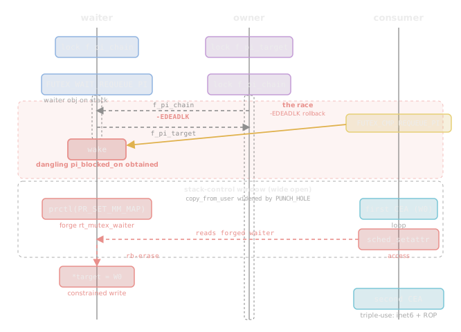
Race windowRace window

The requeue tries to proxy the waiter onto f_pi_target. The owner of f_pi_target is already blocked behind the waiter through f_pi_chain, so the chain walk closes the loop waiter -> f_pi_target -> owner -> f_pi_chain -> waiter. It returns -EDEADLK and takes the buggy rollback. The waiter wakes with a dangling pi_blocked_on.

Here the only ordering that matters is the requeuer rolling back the waiter while the waiter still owns the soon-to-be-freed object, and once the cycle is staged that happens on its own. After it resolves there is no time pressure at all. The waiter sits in userspace with a dangling pi_blocked_on, and the follow-up sched_setattr() that walks the chain can fire whenever it likes. The UAF window is wide open.

The catch is where the freed object lives on the kernel stack (stack-UAF if we call ret out of the futex syscall a “free”). To reclaim it, we need to find a syscall that can land controlled bytes back on the same stack at the same depth (offset).

Triggering the stack-UAF

Staging the three-futex cycle leaves the waiter task in userspace with pi_blocked_on dangling into its old FUTEX_WAIT_REQUEUE_PI frame. Everything below rides on that one pointer.

Note that three threads is for better understanding. To win the race and trigger UAF, you only need one CPU core.

The initial primitive from GhostLock

By now we hold a pointer into freed kernel stack, and we can trigger, at will, a kernel access that dereferences it as an rt_mutex_waiter. We can spray controlled bytes onto that stack and forge the rt_mutex_waiter outright. Depending on the layout we forge, this one access yields several primitives, two main ones:

  • write a pointer to an arbitrary (but constrained) address
  • write 8 bytes of zero to an arbitrary (but constrained) address

Several pointer dereferences and integrity checks run before the primitive fires, and after it fires the kernel returns normally, no crash.

So our main questions, each answered in a section below:

  • how do we get the freed stack memory back (spray)? -> Reusing the stack
  • how do we get the fake rt_mutex_waiter past its built-in structural checks, and forge pointers that read as valid? -> From fake waiter to a write
  • which write primitive, and what do we write where? what does the primitive constrain about the “arbitrary” address? -> Use inet6_protos

Exploit Details

Exploit Summary

  • prefetch -> Leak the kernel image slide and the physmap base.
  • GhostLock -> Leave a dangling rt_mutex_waiter in the waiter task’s pi_blocked_on.
  • (stack-)UAF Reclaim -> Use PR_SET_MM_MAP to reclaim the waiter’s own kernel stack and forge a fake rt_mutex_waiter over the freed frame.
  • Arb address writer -> Rtmutex rb-tree erase: one constrained pointer write (which we can reclaim its content), overwrite struct which contains a function table: inet6_protos[IPPROTO_UDP] = <CEA pointer>.
  • CPU entry area -> Host {fake inet6_protocol, pivot slots, ROP stack} all together at a known direct-map address.
  • Trigger CFH -> Trigger a loopback IPv6 UDP packet calls through the overwritten handler and pivots.
  • DirtyMode -> One write flips core_pattern’s mode bits, then the rest LPE is pure userspace.

This part we are focusing on basic exploit steps of generic x86 Linux systems, our next blog will discuss how to exploit GhostLock on Android, reclaiming stack frame, bypassing both ASLR and CFI.

Background of used tricks

Prefetch ASLR Leak

A prefetch on a given address runs in a different number of cycles depending on whether that address is mapped in the current page tables, so an unprivileged process can time prefetch across the kernel range and read off which addresses are mapped (the prefetch paper has the details).

It works here as Linux barely randomizes the base of its default kernel image (~9 bits of entropy for text base), so a little averaging can recover the KASLR base with near 100% reliability.

In theory any CPU with prefetch and without proper Kernel Page-Table Isolation is affected. But in practice it is more of an x86 technique (unless the ARM target runs KPTI off). kernelCTF images keep KPTI disabled.

kernelCTF images keep KPTI disabled, but even with KPTI on, prefetch paired with EntryBleed can still recover the kernel image base through the trampoline.

CEA spray and randomization bypass

The CEA (CPU entry area) is a per-CPU x86 structure holding the stacks and register context used for entry and exception handling: on an exception, interrupt, or syscall the CPU switches to a stack that lives in the CEA, and the entry code spills the register frame (pt_regs) there. An unprivileged userspace program can trigger a software exception and write its own register context into the pt_regs saved on a CEA exception stack. Before 6.2 the CEA sat at a completely fixed address, so we can place about 120 bytes of contiguous controlled memory at a known kernel address, which is very handy for forging structures, for absorbing the side effects of the pointer dereferences along the way, and for staging a ROP stack.

After Project Zero’s Bringing back the stack attack writeup, the kernel started strongly randomizing the CEA’s virtual address (since 6.2). But the virtual address of the CPU entry area is never needed, as the CEA’s physical offset is fixed, so its direct-map alias follows from the physmap base (same observation @kqx used).

That direct-map address is easy to leak with prefetch, plus candidate-edge normalization and a check against the predicted CEA page to reject neighbouring aliases. (The direct-map leak is noisier than the text one and may need a little more tuning, but it lands at very high accuracy on the target in the end.) So we can always compute the CEA’s other virtual-address mapping:

cea_direct = physmap_base + CPU1_CEA_BASE

Note that each CPU’s CEA virtual address is randomized to a different place. Their physical addresses are all fixed, though, and this offset depends mainly on the target’s kernel version and boot memory size. In the kernelCTF LTS 6.12.80 3.5G-boot environment, it is 0x11c517000(+0x1f58).

Reusing the stack: forging the waiter with PR_SET_MM_MAP

The dangling object is the waiter’s own stack rt_mutex_waiter.

struct rt_mutex_waiter {
  struct rt_waiter_node tree;     // rb node, lives in lock->waiters
  struct rt_waiter_node pi_tree;
  struct task_struct *task;
  struct rt_mutex_base *lock;
  unsigned int wake_state;
  struct ww_acquire_ctx *ww_ctx;
};

Controlled bytes have to land back over that exact frame, on the waiter thread’s own stack, and stay there long enough to be read. The waiter thread returns from the futex syscall and immediately calls prctl(PR_SET_MM, PR_SET_MM_MAP, ...). Inside, prctl_set_mm_map() copies a user-supplied auxv into a fixed-size unsigned long user_auxv[AT_VECTOR_SIZE] stack buffer. That buffer sits at roughly the same stack depth as the freed waiter, so it is a large, naturally-aligned, namespace-free block of controlled qwords landing right on top of the old object.

The auxv is laid out so the overlapping qwords become:

  • tree, an rb node crafted so erasing it promotes one chosen child pointer (W0_BASE, below) into the tree root.
  • task, set to &init_task, a valid task_struct so the chain walk’s task derefs are safe.
  • lock, set to &inet6_protos[IPPROTO_UDP] - 8, the write target.
  • wake_state, set to 0.

The auxv is backed by a memfd and positioned so the copy straddles a page boundary. A sibling thread races fallocate(PUNCH_HOLE) on the trailing page during the prctl, which stretches the copy_from_user window. The forged waiter stays live on the stack while, on another CPU, a consumer thread fires sched_setattr() on the waiter to walk the PI chain.
The race window is wide and we believe GhostLock is also exploitable on a single-core CPU.

clone/setsockopt/pselect/keyctl and other syscalls with large controlled stack locals work the same way. prctl is just convenient here. The buffer is large, aligned, and needs no namespace.
Here’s more useful syscalls that can reclaim the stack frame in our open-sourced PoC code.

From fake waiter to one controlled (limited) write

Controlling the waiter does not give an arbitrary write. The chain walk only does:

task->pi_blocked_on -> fake waiter
fake waiter->lock    -> fake rt_mutex_base
rt_mutex_dequeue(lock, waiter)        // rb_erase on lock->waiters

rt_mutex_dequeue() is an rb-tree erase, and erasing a single-child root writes that child into the root slot. Pointing lock at target - 8 lines the rt_mutex_base fields up over the data around the target pointer.

target - 8  ->  raw_spinlock_t wait_lock        (must read as "unlocked")
target      ->  waiters.rb_root.rb_node          (this slot gets written)
target + 8  ->  waiters.rb_leftmost
target + 16 ->  owner

The fake waiter’s rb node is crafted so the erase writes exactly one child pointer into rb_root.rb_node. The write primitive itself is a single constrained store: *(uint64_t *)target = W0_BASE.

The constraints are also highly strict: The qword before the target must read as an unlocked spinlock, meaning zero in the low 4 bytes, or the trylock fails and the walk exits without writing. The qwords after it (rb_leftmost, owner) must not steer the walk into an uncontrolled top waiter or owner. An unmapped value there faults and panics the box. The equivalent target address constraint is roughly as follows (*target will be written to a pointer):

*(u32 *)(target - 0x08) == 0
*(u64 *)(target + 0x08) == 0 // simplified
((*(u64 *)(target + 0x10)) & ~1ULL) == 0
// Then we can do:
*(u64 *)target = &W0->tree.entry  // W0_BASE

Here the W0_BASE has to point at something that stays valid through the comparisons and the no-owner wakeup later in the same rt_mutex_adjust_prio_chain(). We point it at the direct-map alias of the CPU entry area, which pays off twice:

  • Before the write: the CEA is controllable memory at a known address, so we can forge a self-consistent fake waiter and lock at W0 that survives the walk.
  • After the write: the target now points into the CEA. Once the walk is over, W0 no longer has to look like a waiter at all, so we can re-spray the CEA with whatever the kernel expects the target to point at (if we overwritten a function table pointer with W0, we can now fake function pointer in CEA to get Control Flow Hijack).

Why the CEA?

There’s several ways to spray controlled memory at a fixed (knowned) kernel address. The CEA is one of the more efficient, and its main limit is the ~120-byte small size. NPerm, kernelsnitch and other tricks can do the same job with more room.

Before the trigger, W0 is spraied as that fake waiter and lock pair: task = &init_task, a legit prio, and a lock whose wait_lock reads unlocked and whose owner is benign, so the dequeue, re-enqueue, priority update and wakeup all survive.

The following figure shows how CPU entry area is used to first hold fake rt_mutex_waiter and lock structures, then serve inet6 (next section), ROP stack and JOP gadgets for stack pivoting at the same time, and eventually use a very short ROP to perform the DirtyMode and safely halt the core.
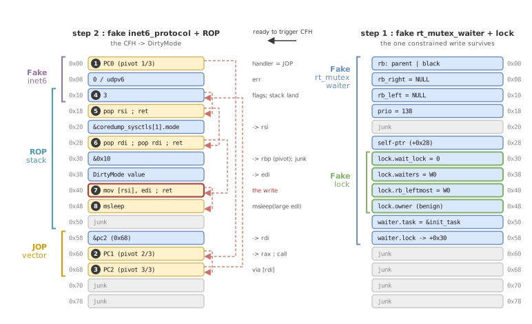
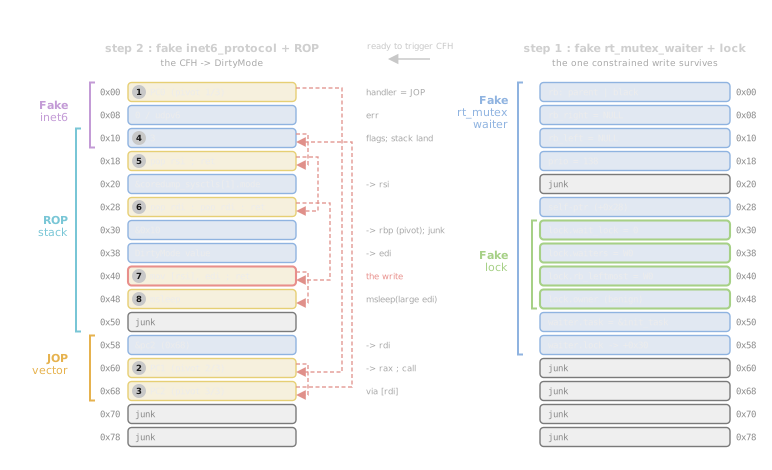
Dual use of the CEA, with three data structures overlapped within 104 bytesDual use of the CEA, with three data structures overlapped within 104 bytes

Use inet6_protos[IPPROTO_UDP] to help

Start from now the exploit path would differ from targets, as of regular x86_64 Linux kernel, we can pick a shorter path by just overwriting some function table (or any object that contains one), as we already have KASLR leaked and ready to get a CFH.

A scan of writable data turns up many pointer tables whose neighbours satisfy the layout above. inet6_protos[IPPROTO_UDP] is a nice one. The neighbours fall out for free, and the trigger is a trivial unprivileged loopback packet.

inet6_protos[16]  == NULL              // fake wait_lock -> unlocked
inet6_protos[17]  == &udpv6_protocol   // <- target (IPPROTO_UDP)
inet6_protos[18]  == NULL              // fake rb_leftmost
inet6_protos[19]  == NULL              // fake owner

After the write, inet6_protos[IPPROTO_UDP] points into the CEA page, where the kernel expects an inet6_protocol.

struct inet6_protocol {
  int (*handler)(struct sk_buff *skb);
  int (*err_handler)(...);
  unsigned int flags;
};

So W0 is re-spraied as a fake inet6_protocol. handler is the first pivot gadget, err_handler is unused, and flags is INET6_PROTO_NOPOLICY | INET6_PROTO_FINAL. Once we send a loopback IPv6 UDP (connect then write to ::1), the kernel will dereference the handler and give us a PC control.

The pivot and DirtyMode

We use the same compact CEA window to holds multiple objects: {the fake inet6_protocol, a few JOP/pivot slots, the final ROP stack}. On Google’s lts-6.12.80 kernel target we are not lucky enough to find a nice single stack pivot target, so the chain takes one extra load/call to land the CEA address in rbp, then pivots with mov rsp, rbp; pop rbp; ret.

A ret2usr or a full /proc/%P/fd/x overwrite would run to around ten gadget qwords, which is too long. So we use DirtyMode as the final exploit stage: a single write, with an almost-garbage value, that flips a permission bit. After it, LPE can be done purely in userspace.

Here we target at the core_pattern sysctl’s mode flags:

static struct ctl_table coredump_sysctls[] = {
  ...
  { .procname     = "core_pattern",
    .data         = core_pattern,
    .maxlen       = CORENAME_MAX_SIZE,
    .mode         = 0644,
    .proc_handler = proc_dostring_coredump },
  ...
};

coredump_sysctls lives in writable kernel data (share same KASLR slide with kernel image). The ROP writes a permissive value to coredump_sysctls[1].mode. Any value with the write bit (2nd LSB) set is enough.

Here we uses a short pop reg; mov [reg], reg; ret plus an msleep to park the hijacked thread safely. And now /proc/sys/kernel/core_pattern is now world-writable, so an unprivileged process opens it, writes |/proc/%P/fd/666 %P, and crashes a helper to trick kernel runs our binary as root.

The initial write primitive (the rb-tree write) cannot reach coredump_sysctls[1].mode directly because of where it lands, so the mode flip is done from the short ROP stage.

Appendix

The full exploit code can be found in our open source security research project, CyberMeowfia.

bigger ROP or NPerm

kernelCTF is a race, and the shortest reliable chain wins. NPerm-backed memory makes a fine large fake stack after the hijack, and there are heavier routes that would also work, including Lukas Maar’s heap-KASLR leak. Each adds another stage and increases time cost. CEA plus DirtyMode is the shortest path to a one-write win, and on the remote it win us the flag in about 5 seconds.

Mitigation

The patch

diff --git a/kernel/locking/rtmutex.c b/kernel/locking/rtmutex.c
--- a/kernel/locking/rtmutex.c
+++ b/kernel/locking/rtmutex.c
@@ -1544,6 +1544,8 @@ static bool rtmutex_spin_on_owner(struct rt_mutex_base *lock,
  *
  * Must be called with lock->wait_lock held and interrupts disabled. It must
  * have just failed to try_to_take_rt_mutex().
+ *
+ * When invoked from rt_mutex_start_proxy_lock() waiter::task != current !
  */
 static void __sched remove_waiter(struct rt_mutex_base *lock,
           struct rt_mutex_waiter *waiter)
@@ -1551,14 +1553,15 @@ static void __sched remove_waiter(struct rt_mutex_base *lock,
 {
   bool is_top_waiter = (waiter == rt_mutex_top_waiter(lock));
   struct task_struct *owner = rt_mutex_owner(lock);
+  struct task_struct *waiter_task = waiter->task;
   struct rt_mutex_base *next_lock;
 
   lockdep_assert_held(&lock->wait_lock);
 
-  raw_spin_lock(&current->pi_lock);
-  rt_mutex_dequeue(lock, waiter);
-  current->pi_blocked_on = NULL;
-  raw_spin_unlock(&current->pi_lock);
+  scoped_guard(raw_spinlock, &waiter_task->pi_lock) {
+    rt_mutex_dequeue(lock, waiter);
+    waiter_task->pi_blocked_on = NULL;
+  }
 
   /*
    * Only update priority if the waiter was the highest priority
@@ -1594,7 +1597,7 @@ static void __sched remove_waiter(struct rt_mutex_base *lock,
   raw_spin_unlock_irq(&lock->wait_lock);
 
   rt_mutex_adjust_prio_chain(owner, RT_MUTEX_MIN_CHAINWALK, lock,
-           next_lock, NULL, current);
+           next_lock, NULL, waiter_task);

We had also sent a fix to security@kernel.org before v1 landed. Its core:

static void __sched remove_waiter(struct rt_mutex_base *lock,
          struct rt_mutex_waiter *waiter)
          struct rt_mutex_waiter *waiter,
          struct task_struct *task)
{
  ...
  raw_spin_lock(&current->pi_lock);
  raw_spin_lock(&task->pi_lock);
  rt_mutex_dequeue(lock, waiter);
  current->pi_blocked_on = NULL;
  raw_spin_unlock(&current->pi_lock);
  if (task->pi_blocked_on == waiter)
    task->pi_blocked_on = NULL;
  raw_spin_unlock(&task->pi_lock);
  ...
  rt_mutex_adjust_prio_chain(owner, RT_MUTEX_MIN_CHAINWALK, lock,
           next_lock, NULL, current);
           next_lock, NULL, task);
}

Instead of reading the task out of waiter->task, the callers pass in the owning task (current on the self-blocking path, the proxied task on the rt_mutex_start_proxy_lock() rollback), and pi_blocked_on is cleared only when it still points at this waiter. task is always a valid task and the clear is guarded.

RANDOMIZE_KSTACK_OFFSET

The stack-reuse step relies on the freed waiter frame and the later user_auxv frame overlapping deterministically. With RANDOMIZE_KSTACK_OFFSET on they no longer do, and the step becomes a roughly 1/32 (5-bit) stack-offset guess. Both submitted targets leave it off by default. The mitigation target turns it on, so this path was not used there.

STATIC_USERMODE_HELPER

STATIC_USERMODE_HELPER would close this particular DirtyMode path. But the same idea can be generalized to any /proc/sys knob whose ctl_table::mode gates access and whose table sits in predictable writable kernel data.

Timeline

  • 2026-04-18: We reported the bug and sent a draft patch to security@kernel.org.
  • 2026-04-20: The bug was fixed with another patch.
  • 2026-05-04: The fix v1 was backported.
  • 2026-06-30: Google acknowledged our kernelCTF submission.
  • 2026-07-07: We published this blog post.

Disclosure policy

For all bugs found by VEGA, we follow our standard 90+30 days disclosure policy as described on our About page.
The Daily Front Page 25 of 26
Monday, July 13, 2026 The Daily Front No. 5 — Colophon

That's the Front for Today

Issue No. 5 — Monday, July 13, 2026 — went to press 2026-07-16 at 11:40 UTC.

About This Magazine

The Daily Front is a daily digital magazine assembled from the stories that reached the front page of Hacker News on Monday, July 13, 2026. Headlines, points, and comment counts are recorded as they stood at press time. All articles remain the property of their original authors — every piece links back to its source and its discussion thread.

How It Was Made

Fetched, cleaned, and typeset by an automated pipeline. An editor model laid out the pages, chose the highlights, and briefed the cover illustrator — 28 model calls and 232k tokens in total. Set in Jacquard 12, Playfair Display, Source Serif 4, and IBM Plex Mono, all served via Google Fonts under the SIL Open Font License.

The Cover

The cover illustration was commissioned with this prompt:

Create a surreal neo-baroque glass mosaic and stained-glass artwork in portrait orientation. The scene is a dim operations room at dawn, but rendered as luminous fragments of colored glass rather than ink or newspaper etching. An open server rack stands like a dark cathedral cabinet, its panels made of obsidian and smoky blue glass. From it, a translucent ghost made of frosted glass and pale opal shards drifts outward, dissolving into tiny pixel-like tesserae.

Beside it, a brass automaton clerk with jointed porcelain hands kneels on a reflective tiled floor, accidentally spilling private folders, old keys, and glowing cipher-like shapes — but none of the shapes contain readable text. The folders are abstract planes of amber and burgundy glass. The keys gleam in metallic gold mosaic pieces.

In the background, tall arched windows reveal a restless red ocean at dawn, glowing like molten stained glass beneath a bruised violet sky. Outside in the rain, a lonely street-pole surveillance camera hangs unplugged, its cable curling like a black ribbon. The rain is shown as vertical silver glass rods catching the first morning light.

Art style and medium: contemporary stained-glass mosaic fused with Byzantine icon aesthetics and Art Nouveau curves​, luminous lead lines, jewel-toned translucent glass, gold leaf accents, fractured reflections, iridescent surfaces, sacred-but-technological atmosphere. Palette of deep cobalt, smoky violet, ruby red, tarnished gold, opal white, and pale dawn cyan. Highly dramatic, elegant, strange, museum-quality, cinematic, ornate yet clean, with strong silhouette and beautiful negative space.

Production Ledger

StageModelCallsTokens InTokens Out
extractgpt-5.5 27 146,692 63,846
layoutgpt-5.5 1 18,687 3,082

The Publisher

Published by Johnny.

Support the Press

If The Daily Front brightens your morning, consider supporting its publisher.

Credits & Contact

All content — articles, posts, comments, and the images within them — belongs to its original authors and is reproduced here to point readers back to the source. Full credit goes to those creators; every item links to its original and its Hacker News discussion.

If you are an author and would like your content removed from an issue, write to hi@johnnys.page and it will be taken down.

Feedback is always welcome at the same address: hi@johnnys.page.

Credit where credit is due.

Every page of this issue began as someone else's work — these are the original sources, linked in full.

  1. GhostLock, a stack-UAF that has existed in all Linux distributions for 15 years by ranger_danger — nebusec.ai·HN discussion ↗
  2. Ask HN: Add flag for AI-generated articles by levkk — news.ycombinator.com·HN discussion ↗
  3. Zig Creator Calls Spade a Spade, Anthropic Blows Smoke by crowdhailer — raymyers.org·HN discussion ↗
  4. Samsung Health app threatens data deletion if users opt out AI training by bundie — neow.in·HN discussion ↗
  5. Grok CLI uploaded the whole home directory to GCS by denysvitali — twitter.com·HN discussion ↗
  6. Grok uploaded my user directory to xAI's servers by tnolet — twitter.com·HN discussion ↗
  7. Telegram's t.me domain has been suspended by Tiberium — whois.com·HN discussion ↗
  8. Building and shipping Mac and iOS apps without opening Xcode by speckx — scottwillsey.com·HN discussion ↗
  9. Apple's new SpeechAnalyzer API, benchmarked against Whisper and its predecessor by get-inscribe — get-inscribe.com·HN discussion ↗
  10. A graph that should be front-page news by rakel_rakel — lyrebirddreaming.com·HN discussion ↗
  11. Former NOAA employees built Climate.us to preserve climate data and resources by benwerd — 19thnews.org·HN discussion ↗
  12. LAPD lets contract with surveillance giant Flock expire by forks — techcrunch.com·HN discussion ↗
  13. Sam Neill has died by j4mie — theguardian.com·HN discussion ↗
  14. The art and engineering of Sega CD Silpheed by ibobev — fabiensanglard.net·HN discussion ↗
  15. Linux on the Sega 32X. Who needs hardware synchronization primitives anyway? by cakehonolulu — cakehonolulu.github.io·HN discussion ↗
  16. Designing and assembling my first PCB by tadasv — vilkeliskis.com·HN discussion ↗
  17. Benchmarking 15 “E-Waste” GPUs with Modern Workloads by eso_logic — esologic.com·HN discussion ↗
  18. Show HN: I implemented a neural network in SQL by alxmrs — github.com·HN discussion ↗
  19. Show HN: DOM-docx – HTML to native, editable Word docs (MIT) by fishbone — github.com·HN discussion ↗
  20. Backtrack-Free Cursive by dmit — mmapped.blog·HN discussion ↗
  21. The social physics of conversation: Communication patterns matter by kiyanwang — andiroberts.com·HN discussion ↗
  22. Interrail: 6,379Km and 13 Countries over 7 weeks by coinfused — shkspr.mobi·HN discussion ↗
  23. TFTP Honey Pot Results by speckx — bruceediger.com·HN discussion ↗
  24. Cyberpunk Comics, Manga and Graphic Novels by zdw — shellzine.net·HN discussion ↗
  25. A voxel Tokyo in real Japan time – ride the Yamanote line and study Japanese by momentmaker — jivx.com·HN discussion ↗
  26. Ancient Roman Board Game by nobody9999 — ludus-coriovalli.web.app·HN discussion ↗
  27. Beavis Ultrasound PnP ISA Sound Card Replica by mariuz — github.com·HN discussion ↗
  28. Show HN: YouTube Guitar Tab Parser by neogenix — github.com·HN discussion ↗
  29. Are you telling me a readonly property is wrecking my performance? by forthwall — shub.club·HN discussion ↗
  30. GhostLock, a stack-UAF that has existed in all Linux distributions for 15 years by djfergus — nebusec.ai·HN discussion ↗

Browse all issues in the archive →