Cover illustration

TheDaily Front

Issue No. 2 Saturday, July 11 2026 #2 — SATURDAY, JULY 11, 2026
All the news that fits in orbit, in court, and occasionally in SQLite.
Saturday, July 11, 2026 The Daily Front No. 2 — Contents
30stories
7,178points
4,838comments
245kllm tokens
Assembled with 30 model calls — 173,883 tokens read, 71,369 written.

Highlights

Apple sues OpenAI, accuses ex-employees of stealing trade secrets

Apple’s trade-secret suit against OpenAI turns the AI talent war into a courtroom spectacle with billions and reputations at stake.

Nvidia, CoreWeave, and Nebius: Inside the Circular Financing of the GPU Boom

A deep dive into Nvidia, CoreWeave, and Nebius asks whether the GPU boom is building durable infrastructure—or financing its own demand.

SpaceX wants to launch 100k more Starlink satellites for 100x the bandwidth

SpaceX’s proposed 100,000-satellite Starlink expansion promises bandwidth enough for the hinterlands and controversy enough for the heavens.

Einstein's relativity rules chemical bonds in heavy elements, new research shows

Brown chemists report direct evidence that relativity reshapes chemical bonding in heavy elements, unsettling a tidy textbook picture.

RISCBoy is an open-source portable games console, designed from scratch

RISCBoy delivers the day’s most charming maker marvel: an open-source handheld console from a parallel RISC-V past.

From the Editor

Today’s front page finds the modern machine age arguing with itself: Apple drags OpenAI to court, GPU money chases its own tail, and SpaceX asks for a sky thick with hardware. Yet beneath the thunder, our quieter columns remind us that progress still lives in craft—better databases, homemade consoles, strange clocks, silent speech, and chemistry where Einstein himself has the last word.

  1. Apple sues OpenAI, accuses ex-employees of stealing trade secrets3
  2. Nvidia, CoreWeave, and Nebius: Inside the Circular Financing of the GPU Boom4
  3. SpaceX wants to launch 100k more Starlink satellites for 100x the bandwidth5
  4. AI 2040: Plan A6
  5. Einstein's relativity rules chemical bonds in heavy elements, new research shows7
  6. UPI: Anatomy of a Payment Transaction8
  7. We scaled PgBouncer to 4x throughput9
  8. Prefer strict tables in SQLite10
  9. ZeroFS vs. Amazon S3 Files11
  10. Preemption is GC for memory reordering (2019)12
  11. RISCBoy is an open-source portable games console, designed from scratch13
  12. Biff.graph: structure your Clojure codebase as a queryable graph14
  13. An iroh powered smart fan15
  14. Show HN: Orbit – AR satellite tracker, watch 15k+ objects16
  15. Silent speech with ultrasound17
  16. Modern decor may be straining people's brains18
  17. Female US rower completes historic solo journey from California to Hawaii19
  18. Leaded gas was a known poison the day it was invented (2016)20
  19. Optimization Solver as a Service21
  20. Show HN: Ant – A JavaScript runtime and ecosystem22
  21. Show HN: Learn by rebuilding Redis, Git, a database from scratch22
  22. Amber the programming language compiled to Bash/Ksh/Zsh22
  23. Otary – Image and Geometry Python Library Now Has Tutorials22
  24. The early History of the Singular Value Decomposition (1993) [pdf]23
  25. Alternate clock designs and time systems23
  26. Book: RISC-V System-on-Chip Design23
  27. Digital Deli, 1984 book by early PC hackers and enthusiasts23
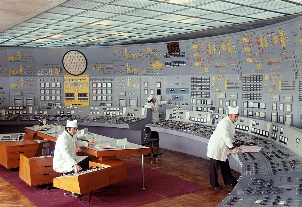
  28. The vintage beauty of Soviet control rooms (2018)24
  29. How to hide from killer drones24
  30. Google Search lets creators know more about their reach24
The Daily Front Page 2 of 25
Saturday, July 11, 2026 The Daily Front No. 2 — The AI Secrets Trial
article

Apple sues OpenAI, accuses ex-employees of stealing trade secrets

by stock_toaster·▲ 1,623 points·932 comments·9to5mac.com ↗
“This case is about Apple’s former employees stealing Apple’s trade secrets for the benefit of OpenAI.”

Apple has filed a lawsuit against OpenAI today, accusing the company of trade secret theft. Specifically, Apple alleges that its former employees have stolen trade secrets “for the benefit of OpenAI.”

“This case is about Apple’s former employees stealing Apple’s trade secrets for the benefit of OpenAI. Apple brings this suit to put a stop to it,” the lawsuit says.

Apple statement

In a statement to 9to5Mac, an Apple spokesperson said:

“At Apple, our teams are constantly developing breakthrough technologies to create the best products and services in the world, and protecting their work and intellectual property is something we take very seriously. Recently, significant evidence has emerged suggesting individuals employed by OpenAI wrongfully took Apple’s secret and confidential information regarding our unreleased technologies, processes, and products. We will always defend our teams’ hard work and innovations, and we are taking all appropriate steps to do so.”

Update: Read OpenAI’s response here.

Apple accuses OpenAI of trade secret theft

The lawsuit names Chang Liu and Tang Tan as two of the defendants. Tang Tan served as VP of product design at Apple, leading iPhone and Apple Watch product design. He departed the company in February 2024 to work with Jony Ive. Chang Liu, meanwhile, worked at Apple for eight years and was a senior system electrical engineer before departing to join OpenAI in January 2026.

Apple’s lawsuit also names OpenAI and io Products as defendants.

OpenAI’s hardware efforts are being led by Jony Ive, Apple’s former chief design officer. OpenAI acquired Ive’s startup io as part of a $6.5 billion deal last year. OpenAI’s takeover of the company included more than 50 engineers, developers, and other employees. In its original announcement, OpenAI touted that Ive founded io in collaboration with Scott Cannon, Evans Hankey, and Tan.

Hankey led Apple’s design team for several years after Ive departed the company. She departed in 2022 before reuniting with Ive as part of io. Cannon also previously worked at Apple.

Ive, Hankey, and Cannon are not personally mentioned anywhere in Apple’s initial filing today.

The complaint

Apple says it first raised concerns with OpenAI directly in February, asking the company to investigate and address the issue. OpenAI, however, never responded. Apple says the conduct detailed in the filing is “the tip of the iceberg.”

This is the tip of the iceberg. Apple lacks visibility into what’s been happening behind closed doors at OpenAI, where such misconduct is normalized and exemplified by leadership. This much is clear, however: at every level, from members of its Technical Staff to its Chief Hardware Officer, and in coordination with business partners, OpenAI has been stealing Apple’s trade secrets and confidential information. As a natural result, OpenAI’s nascent hardware business now rests.

Jony Ive and Sam Altman

The complaint, filed in the U.S. District Court for the Northern District of California, alleges that Tan used insider knowledge of Apple’s confidential projects to grill job candidates in interviews and learn more confidential information. Additionally, Tan directed job candidates still working at Apple to bring actual Apple hardware components and samples for “show and tell” sessions.

When interviewing Apple employees for jobs at OpenAI, Mr. Tan uses Apple’s confidential information to gain access to even more insider knowledge. He has used an Apple internal project codename to ask, “What’s the plan[?]” for an unannounced Apple product.

He has directed job candidates still working for Apple to bring “Actual parts” from Apple to their interviews for “show and tell” sessions in which he and his team at OpenAI can elicit still more Apple confidential information. These directions to bring Apple’s parts to OpenAI job interviews surprised at least one of the candidates, who commented that he “didn’t even know we could take those from the office.”

OpenAI has been instructing Apple employees to bring “CAD/design artifacts” and “prototypes” to their interviews and to divulge details about their work such as “subsystem and component selection,” the “tools or methodologies you use for system integration, such as CAD software, simulation tools,” and “Vendor selection and communication/collaboration with vendors.”

Furthermore, Apple says a candidate began “screenshotting and downloading files relating to a highly confidential Apple project” hours before interviewing with Tan, who then “solicited more information about that same Apple project” once the interview started. This became an “established pattern,” Apple says.

Tan also allegedly possessed and distributed an internal Apple “Need to Know” document to new OpenAI hires before they gave their notice to Apple. The document included Apple’s departure security protocols. As part of its investigation, Apple found a “pattern by employees who depart for OpenAI of taking steps to evade the security processes intended to protect Apple’s confidential information.”

Meanwhile, Apple also claims former engineer Liu exploited a security bug to download confidential engineering files after leaving the company. Rather than report the exploit, Liu allegedly joked about it in messages (“LOL,” “so funny”). Liu also failed to return an Apple-issued laptop after his departure.

Apple alleges that Liu downloaded a “compilation of technical files with over a thousand pages” with details of work he did at Apple. This included detailed manufacturing documents covering the complex circuit boards used in Apple hardware products.

Liu also allegedly coached another Apple employee at the time, whom he was recruiting to OpenAI, on which confidential materials to study before her own OpenAI interview.

Finally, Apple alleges that OpenAI had a trusted Apple partner carry out Apple’s proprietary metal-finishing technique, misleading the partner into believing it had Apple’s permission to do so. Apple also says OpenAI approached a second longtime Apple supplier that works on power and battery manufacturing, using insider terminology to ask “targeted questions” about specific Apple components.

The suit seeks injunctive relief and damages, and comes as OpenAI works to bring its first consumer hardware device to market.

Apple’s lawsuit also comes after Bloomberg reported that OpenAI was preparing “legal action” against Apple over how its partnership to integrate ChatGPT into Siri played out. Today’s lawsuit from Apple, however, says that agreement is not at issue here.

Tan and Liu are just two of many Apple employees who have departed for OpenAI. Today’s filing says that there are over 400 former Apple employees now working at OpenAI.

There have been various rumors about OpenAI’s hardware efforts so far. In April, Ming-Chi Kuo reported that OpenAI is developing its own smartphone, which could launch in 2028. The Information has also reported on OpenAI’s work on a HomePod-style smart speaker.

You can read the full filing below and find the PDF linked here.

Apple Inc. v. Liu et alDownload

The Daily Front Page 3 of 25
Saturday, July 11, 2026 The Daily Front No. 2 — The GPU Money-Go-Round
article

Nvidia, CoreWeave, and Nebius: Inside the Circular Financing of the GPU Boom

by adletbalzhanov·▲ 355 points·155 comments·io-fund.com ↗
“CoreWeave’s and Nebius’ growth is far from profitable, as they seek to capture AI demand.”
  • Neoclouds are seeing massive hyperscaler demand as companies race to scale AI infrastructure, resulting in rapid revenue and backlog growth.
  • Leaders like CoreWeave and Nebius enable this through access to the latest Nvidia GPU’s while also optimizing compute utilization.
  • However, the bearish argument behind hyperscaler demand lies in their desire to offload their capex spending and shift costs to the operating expense line.
  • CoreWeave’s and Nebius’ growth is far from profitable, as they seek to capture AI demand with limited cash flow and soaring debt loads in an increasingly tough macro backdrop.
  • Circular financing, demonstrated by Nvidia’s investments and financial backstopping, is another key item to monitor closely

Neoclouds are one of the more hotly debated AI business models, with CoreWeave and Nebius being the two most widely recognized names. These companies have seen their sales, backlog, and share prices soar, differentiating themselves through quick access to the latest GPU compute and GPU utilization advantages that allow hyperscalers to rapidly add efficient compute capacity. 

Notably, CoreWeave and Nebius have each secured 3.5 GWs of contracted power capacity; while these power footprints are key considering power is a hindrance to data center expansion, the vast majority of their contracted power capacity has yet to come online. CoreWeave is targeting 1.7 GW of active power by the end of 2026, while Nebius is targeting 800 MW to 1 GW of connected power. 

In turn, they are quickly working to convert their contracted power to active power, and thus convert large backlogs into revenue. Yet doing so is extremely expensive, and neoclouds do not have the same cash nor operating cash flow profiles of Big Tech. This is leading neoclouds to employ unique and circular financing structures, raising some red flags. 

In this analysis, I dive into the two public neoclouds that are riding Nvidia equity, hyperscaler contracts, and GPU-backed debt to fund the buildout, and what it means for the durability of the surge. 

Microsoft and Meta’s $120B+ Bet on Neoclouds

The size of hyperscaler-neocloud partnerships compared to their current revenue is astounding. Microsoft has struck the most neocloud deals, with approximately $60 billion worth of commitments between CoreWeave, Nebius, and other private players such as Nscale. Meanwhile, Meta has committed $35.2 billion to CoreWeave in total after its recent $21 billion expansion, and an up to $27 billion deal with Nebius for a total commitment of up to $62.2 billion. Along with Meta, OpenAI is one of CoreWeave’s two largest customers, while CoreWeave also has a multi-year compute agreement with Anthropic.  

Alone, Microsoft and Meta’s total commitments extend up to $122.2 billion – for perspective, that is ~90% of the TTM revenue of AWS being allocated towards neoclouds over long-term capacity deals. When factoring in hyperscaler-backed deals from OpenAI and Anthropic (although exact deal value is unknown), total potential commitments surpass $145 billion.  

Keep in mind, CoreWeave’s FY2026 estimated revenue is $12.6B and Nebius FY26 revenue is expected to be $3.4B - therefore, these partnerships are leading to commitments that are an order of magnitude higher than current sales.  

The reason hyperscalers are willing to allocate this capital to a relatively new business model in the neoclouds is three-fold – quick access to leading GPU generations, optimized compute utilization, and the added benefit of not having to recognize capex on the balance sheet – we look at each of these drivers below. 

Neocloud Advantage is Offering Quick Access to GPUs

At its root, neocloud demand is a product of hyperscalers' insatiable demand for compute capacity. However, neoclouds can often add compute capacity much faster than hyperscalers can through internal builds, offering a key value proposition for Big Tech. As hyperscalers spend hundreds of billions a year on AI compute, minimizing the lag between data center expenses and revenue generation is critical to maximizing their return on investment. 

Supporting the argument around neocloud’s advantage lying within time to deployment, commercial real estate giant JLL notes, “Neoclouds can deploy high-density GPU infrastructure within months compared to multi-year builds for hyperscale data centers, providing crucial time-to-market advantages for businesses needing rapid AI development.”

In CoreWeave’s S-1 Registration filing, it lists “Faster access to the latest AI infrastructure advancements” as one of its key benefits to customers. Specifically, CoreWeave says “we were among the first to deliver NVIDIA H100, H200, and GH200 clusters into production at AI scale, and the first cloud provider to make NVIDIA GB200 NVL72-based instances generally available. We are able to deploy the newest chips in our infrastructure and provide the compute capacity to customers in as little as two weeks from receipt.”  

Nebius makes a similar statement in its Annual Report, noting its “consistent track record of being one of the first to deploy the latest generation of NVIDIA GPU chips.” 

CoreWeave and Nebius' relationship with Nvidia is key to acquiring the latest GPUs ahead of others. Nvidia recently invested $2 billion in both CoreWeave and Nebius. Under these partnerships, CoreWeave and Nebius will each look to deploy more than 5 GW of data center capacity by 2030. 

CoreWeave recently demonstrated its ability to offer quick access to the latest chips and newest architectures to hit the market once again, being the first to have a Vera Rubin system up and running at the start of June.  This provides evidence that partnering with CoreWeave and Nebius can help hyperscalers access as much of the latest GPU compute as possible in short order. 

Beyond Hardware: Neocloud Platforms Offering Higher GPU Utilization

Aside from raw compute access, CoreWeave and other neoclouds layer on software and additional capabilities that improve GPU utilization – a key value add for hyperscalers.  

For example, CoreWeave Kubernetes Service (CKS) helps coordinate the allocation of workloads across thousands of GPUs, while its SUNK service helps optimize GPU utilization by allowing training and inference workloads to run on the same cluster. CoreWeave Tensorizer enables high-speed model loading, reducing GPU idle time. 

Combining these software and optimization capabilities with rapid fault detection and remediation services, CoreWeave believes it can offer higher GPU utilization rates than hyperscalers, based on the model FLOPs utilization (MFU) metric. The “MFU gap” is a metric that describes the gap between compute capacity and usage, which today often ranges between 30% to 40%. 

The MFU gap can become quite costly as it represents a more realistic way to measure the performance of GPUs -- rather than only taking into account if a GPU is sitting idle or not. According to Trainy AI: “GPU Utilization is only measuring whether a kernel is executing at a given time. It has no indication of whether your kernel is using all cores available, or parallelizing the workload to the GPU’s maximum capability.”  

Chart showing AI model FLOPS utilization with 100% theoretical vs 35–45% observed performance and efficiency gap

Chart comparing theoretical model FLOPS utilization (100%) with observed performance (35%–45%), illustrating a significant efficiency gap in AI workloads. Source: CoreWeave 

When going public, CoreWeave published its MFU rate at 35% to 45%, stating it is 20% higher than competitors, which means other AI data centers had MFU rates more in the 30% range. However, in a March 2025 blog post, CoreWeave noted that it was achieving an MFU of >50% on Hopper GPUs. This ability to stand up next-generation GPU hardware in short fashion combined with improved utilization rates is where the neoclouds’ advantage lies.  

Behind the Balance Sheet: Why Hyperscalers Are Leasing Neocloud Capacity

By leasing compute capacity from neoclouds, hyperscalers shift their cost timeline from being a large upfront capex outflow to an operational expense outflow spread over long-term contracts. The need to spread costs is becoming increasingly evident due to the massive spending hyperscalers are engaged in.  

Although this is the “bear” case on why hyperscalers work with neoclouds—contrasting this with the rationale behind GPU access and utilization is key because one could argue that hyperscalers are quite capable of software optimizations and GPU utilization on their own (in fact, they are the longstanding incumbent here with deep expertise in cloud operations and workload optimizations). 

Take Meta for example. Analysts are currently expecting the company to generate $136 billion in cash from operations in 2026. With its stated capex guidance of $125 billion to $145 billion, the company could easily be free cash flow negative during the year. However, as noted, Meta also has up to $62.2 billion in neocloud agreements. If Meta built the equivalent value of capacity itself, the firm would recognize that spending as balance sheet capex, weighing further on its already pressured free cash flow.  

On the other hand, neocloud agreements add nothing to Meta’s capex, as the costs are recognized as operating expenses over the life of the contracts. Notably, Meta’s contracts with CoreWeave and Nebius extend through 2031-2032, meaning that opex payments could average less than $10 billion annually. 

Looking at Microsoft, we can see a similar situation. In calendar year 2026, the company is guiding for capex of $190 billion, while analyst forecast $200 billion in cash from operations over the same period. If these figures materialize, the company would consume 95% of its OCF on capex. The $60 billion in neocloud agreements, recognized as operating expenses over many years, expands its capacity while keeping that spend off its cash flow statement. 

As hyperscalers offload their capex, neoclouds are the ones taking that capex on—resulting in their massive funding needs.  

Circular Financing: Nvidia’s Role as an Investor, Supplier, and Demand Backstop

Both Nebius and CoreWeave lend some of their advantage to Nvidia, as it is this partnership with the GPU leader that offers them that ability to be among the first providers to stand up and deploy next-gen platforms such as Blackwell Ultra and now Rubin.  

Having Nvidia as a partner also could play a role in helping CoreWeave and Nebius secure funding at much better terms, extending presence and support beyond the hyperscalers to another investment-grade firm with a strong balance sheet and cash flows. Nvidia’s LTM free cash flow was $119 billion, the second highest of any company in the world, only behind Apple. The downside, however, is that Nvidia’s relationship with the two is one of the most identifiable instances of circular financing.  

This stems from the multi-billion-dollar investments that Nvidia has made in CoreWeave and Nebius. Notably, Nvidia’s latest $2 billion investments in each company were not its first. Nvidia’s Q1 2025 13F filing revealed a CoreWeave stake worth $896.7 million at the time, while its Q4 2025 13F revealed a $33 million stake in Nebius. Thus, the investment relationship between Nvidia and these firms extends well beyond one year. 

Furthermore, in the case of CoreWeave, Nvidia has also provided a significant financial backstop against unsold GPU capacity. Under the agreement with an initial value of $6.3 billion, “in instances where [CoreWeave’s] datacenter capacity is not fully utilized by its own customers, NVIDIA is obligated to purchase the residual unsold capacity through April 13, 2032.” In other words, Nvidia is committed to purchasing unsold GPU capacity if CoreWeave is unable to find another buyer. With an initial value of $6.3 billion, there is the potential that the arrangement could become larger over time. 

As Nvidia makes these investments, CoreWeave and Nebius are going right back to Nvidia to purchase large volumes of GPUs - a clear representation of circular financing. By providing a relatively small amount of equity funding, Nvidia secures relationships with these neoclouds that intend to purchase tens of billions' worth of GPUs.  

Nvidia could see long-term benefits by supporting CoreWeave and Nebius through their ramp-up phases where cash flow is deeply negative. If the firms can eventually become self-sustainable, Nvidia would have two large-scale customers that it can continue selling its latest systems to for years to come. However, for the neoclouds, the concern is whether they have to continually raise cash into the foreseeable future to build new infrastructure and when that would level out, as revenue lags capex 2:1. 

How Neoclouds Are Funding AI Expansion: Debt, Equity, and Circular Financing

Both CoreWeave and Nebius are eyeing rapid ramps in active power – CoreWeave currently has 1GW of its 3.5GW contracted power pipeline active, but it aims to convert the majority of that over to active capacity by the end of 2027, while Nebius similarly has 3.5GW of contracted power and a goal of reaching up to 1GW of connected (active or can be activated upon GPU installation) by the end of 2026.  

However, as with all AI buildouts right now, the keywords are “active power” as energy constraints are intensifying across the board.  

CoreWeave’s Balance Sheet Challenged, Debt Quickly Rising

CoreWeave’s balance sheet is in a difficult position, as the company looks to rapidly expand its active power footprint at a rate that is not supported by its cash balance and its operating cash flow. 

Revenue of $2.08 billion rose by 112% YoY in its latest quarter. However, operating cash flows (OCF) came in at $2.98 billion, compared to capex of $7.7 billion, leading to free cash flow of -$4.71 billion. This mismatch led to the firm’s cash balance falling by $890 million, or 28.3% QoQ to $2.27 billion. Meanwhile, debt increased by nearly $3.5 billion, or 16.1% QoQ to $24.86 billion – this is set to rise further in Q2 as CoreWeave just announced a $3.5 billion senior note raise on June 11. 

Line chart showing CoreWeave quarterly capex rising to $7.7B vs revenue at $2.07B in 2026

Chart showing CoreWeave’s quarterly capex rising sharply to approximately $7.7 billion, while revenue reached around $2.07 billion over the same period. Source: YCharts

For the full-year, CoreWeave expects to spend $31 billion to $35 billion on capex, or $33 billion at the midpoint. This implies capex spending for the remainder of the year of $25.3 billion. Analysts currently estimate that the company will generate $8.68 billion in operating cash flow in 2026, or just $5.7 billion for the rest of the year. Given CoreWeave’s $2.27 billion cash balance, this creates a huge funding gap of $17.33 billion. In practice, CoreWeave is likely to raise more than this to avoid further decreasing its already somewhat thin cash cushion. 

CoreWeave has used equity issuance in the past as a funding source, but debt issuance far outweighs this. Looking at its first five earnings reports since going public, its total equity issuance is only $3.5 billion, while debt issuance was more than 5X higher at $18.81 billion. Thus, a further increase in debt is likely to be the primary way that CoreWeave continues to fund its capex plans while already having a net cash position of -$22.6 billion. Looking into its unique funding structures shows that debt will continue to be a key lever that the firm pulls. 

Nebius: Stronger Balance Sheet but Ongoing Funding Needs

Nebius is comparatively in a much better position, with $9.37 billion in cash to $8.45 billion in debt, for a net cash balance of $920 million. Revenue rose 684% YoY to $339 million in its latest quarter, while operating cash flow was $2.26 billion, rising by 170.7% QoQ due to significant customer prepayments. Capex came in at $2.47 billion, resulting in FCF of -$214.9 million.  

However, Nebius is also looking to rapidly expand its active power footprint, with the firm’s midpoint capex guidance for the full year at $22.5 billion. This implies $20 billion in spending over the remainder of the year. Including the company’s cash and contractual commitments of approximately $6.9 billion, Nebius currently needs to draw $6.3 billion in additional funding to support the midpoint of its capex forecast. 

Like CoreWeave, Nebius has also leaned heavily on debt rather than equity issuance to fund itself, although to a lesser extent. Since Q4 2024, Nebius’ total equity issuance was approximately $3.92 billion when including the $2 billion in pre-funded warrants Nvidia recently purchased. Over the same period, its debt issuance was $8.32 billion. In its latest earnings call, Nebius noted asset backed financing, corporate debt, and equity issuance as options for raising capital.  

Notably, Nebius’ undeployed 25 million share at-the-market equity program could go a long way toward bridging its 2026 funding gap. At a $200 share price (around 10% below the stock’s current level), fully utilizing this program would generate gross proceeds of $5 billion while diluting shareholders by approximately 8%. However, given past trends, asset backed and corporate debt are likely to be the primary path forward. 

Overall, this breakdown of CoreWeave and Nebius’ funding requirements for 2026 is just one stage of a much larger push to convert its contracted power into active power. After all this spending, CoreWeave aims to have just under 50% (1.7 GW) of its contracted power active. Meanwhile, Nebius hitting the upper bound of its connected power target would account for less than 30% of its contracted power, which includes power that is either active or can be activated once GPUs are installed.  

In turn, the companies will continue to need to find more and more funding to scale until CFO converges with capex. With the spread between these figures still very wide, the likely result is further increases in debt loads and/or shareholder dilution over several years. 

GPU-Backed Debt: Inside CoreWeave’s Funding Engine for AI Infrastructure

CoreWeave relies heavily on GPU-backed delayed draw term loans (DDTLs), having closed six separate facilities. Under DDTLs, CoreWeave draws down funds intermittently as it uses them to pay for different stages of data center buildouts.  

Notably, the company’s $8.5 billion DDTL 4.0, closed in March, was the first of its kind to receive an investment-grade credit rating. As of Q1 2026, CoreWeave had only drawn $1.26 billion worth of DDTL 4.0. This is the only portion of the $8.5 billion that currently shows up in CoreWeave’s total debt. Thus, as the firm draws down more of DDTL 4.0 over time, its debt will also increase.

Table showing CoreWeave’s debt obligations in Q1 2026, including DDTL 1.0–4.0 facilities, senior notes, and total debt of approximately $25.1 billion, with DDTL 4.0 drawn at $1.26 billion out of $8.5 billion

Table showing CoreWeave’s debt structure with total debt of approximately $25.1 billion, including multiple delayed draw term loan (DDTL) facilities and senior notes. Notably, the DDTL 4.0 facility totals $8.5 billion, but only $1.26 billion has been drawn, indicating significant future debt expansion as capital is deployed. Source: CoreWeave 

CoreWeave notes that the investment-grade rating is “supported by a long-term customer contract with an investment-grade AI enterprise," which is presumably tied to Meta’s latest contract. Essentially, the contract that CoreWeave has signed with the investment-grade customer, as well as the value of the GPUs it buys, are collateral for the debt. This is why the facility can achieve an investment-grade credit rating despite CoreWeave itself having a poor balance sheet, allowing for much more favorable interest rates that CoreWeave could not otherwise receive. 

Still, CoreWeave's ability to receive better interest rates than peers relies on backing from investment grade customer contracts. Notably, DDTL 5.0, closed in May (and is thus not included in the table above), was backed by two non-investment-grade customer contracts. This resulted in the facility not receiving an investment grade rating and thus having a higher interest rate. 

Interest Rate Pressure: A Growing Risk to Profitability

Increases in general rates apply further upward pressure on the rates that CoreWeave and other neoclouds can receive in future funding rounds. The fixed rate tranche of DDTL 4.0 is tied to U.S. Treasuries with an average weighted maturity of 3.14 years, plus a 2% premium. This portion of the yield curve has seen rates rise significantly since the beginning of the year from less than 3.6% to nearly 4.2%.

Line chart showing 3-year U.S. Treasury yield rising from below 3.6% to 4.16% in 2026

Chart showing the 3-year U.S. Treasury rate rising from below 3.6% in early 2026 to approximately 4.16% by June, reflecting a sharp increase in short- to mid-term interest rates. Source: YCharts.

Notably, CoreWeave’s interest payments are already elevated, coming in at $536 million in Q1. This equates to 25.8% of its $2.08 billion in revenue, and 46.3% of its $1.157 billion in adjusted EBITDA. The company is guiding for midpoint revenue of $2.525 billion next quarter, and midpoint interest expense of $690 million—which would push its interest to revenue ratio up to 27.3%. With this, interest expense is expected to become an even more relevant line item while already putting significant pressure on profitability. 

The Neocloud Race: Balancing Surging AI Demand With Rising Debt and Circular Risk

Overall, neoclouds clearly have significant growth momentum, with revenues and backlogs spiking, while attracting interest from investment-grade hyperscalers such as Microsoft and Meta, and AI labs including OpenAI and Anthropic. Access to leading Nvidia systems, and GPU utilization advantages make neoclouds an option for hyperscalers looking to quickly scale AI compute capacity. 

At the same time, the mismatch between operating cash flow and capex is causing debt levels to rise rapidly, which is a dynamic that is unlikely to change in the near term. Elevated interest rates remain an external risk, while circular financing raises questions around the degree to which neocloud growth depends on Nvidia’s capital support, and the extent to which Nvidia’s GPU demand is increasingly tied to the neocloud model.

The Daily Front Page 4 of 25
Saturday, July 11, 2026 The Daily Front No. 2 — A Crowded Sky
article

SpaceX wants to launch 100k more Starlink satellites for 100x the bandwidth

by CrankyBear·▲ 313 points·1,175 comments·zdnet.com ↗
“Starlink’s 100,000 satellites will dwarf existing constellations.”

It could mean faster internet for rural customers, but not everyone is happy.

starlink rocket with satellite

ZDNET's key takeaways

  • Starlink's 100,000 satellites will dwarf existing constellations.
  • When deployed, SpaceX promises the network will deliver gigabit speeds.
  • When it comes to satellite internet, Starlink has no real competition.

Do you like Starlink internet? If so, you'll love that its parent company, SpaceX, has applied to the Federal Communications Commission (FCC) for permission to launch 100,000 third-generation (Gen3) Starlink satellites. The upshot for users? SpaceX promises to deliver "ultra-low-latency" multi-gigabit symmetrical broadband.

Now, I'll believe that when I see it. Today's advertised peak is "up to" around 300 to 400+ Mbps down, but typical real-world speeds are much lower. Over at ZDNET's sister publication, PCMag, reviewer Brian Westover found that even on Starlink's top home plan, the Residential Max plan, mean download speeds plateaued in the 145 megabits per second (Mbps) to 170 Mbps range, with upload speeds of just under 40 Mbps.

Also: I built my own Wi-Fi router with a Raspberry Pi for Starlink and solar control - here's how

That's plodding compared to my home AT&T Internet fiber, which, day in and day out, delivers 2.1 gigabits per second (Gbps) download and upload speeds. I never would have dreamed of such speeds when I was still using a 300-baud modem. But these days, almost no one uses modems, and if you're not living in a broadband-rich area, you may not have access to fiber internet. For people like Westover, who lives in rural Idaho, Starlink isn't just great; it's a necessity.

SpaceX's Gen3 filing

In its FCC application, SpaceX seeks authority to deploy a Gen3 Starlink system in very low Earth orbit (LEO). The filing positions Gen3 as a successor and expansion beyond the existing Gen1 and Gen2 constellations. Today, there are nearly 11,000 Starlink satellites in orbit. If approved, Starlink will launch and operate 100,000 satellites.

These Gen3 satellites will weigh more than 2,000 kilograms, or over two tons. That means SpaceX won't be able to launch a meaningful number of satellites at once using its workhorse Falcon 9 rockets. Instead, CEO Elon Musk has said SpaceX will need to use Starship, which still isn't ready for prime time. In the meantime, Falcon Heavy rockets would be able to launch sufficient Gen3 satellites to deliver the service.

SpaceX has told the FCC that the Gen3 network is intended to serve not only consumers and enterprises but also government customers and "billions of AI-powered devices worldwide," tying the constellation directly to projected compute and data-transport demands from large-scale AI systems. This is no AI data center in space, but it's a step in that direction.

Massive spectrum request

The application seeks access to an unusually broad span of spectrum, including Ku-, Ka-, V-, E-, W-, and D-band frequencies. Downlink bands cited in the filing include 10.7 to 13.4 GHz, 17.3 to 21.2 GHz, and 37.5 to 42.5 GHz, while uplink bands span multiple ranges up to approximately 231.5 to 275 GHz. SpaceX requests waivers of FCC rules, such as Section 2.106, to assemble larger contiguous channels for high-capacity fronthaul, backhaul, and massive uplink.

Also: This 3-in-1 adapter for the Starlink Mini made all the difference for its power delivery

All this means Gen3 could interfere with rival satellite internet services and other wireless services. SpaceX promises to operate on a noninterference, nonprotected basis and to engage in "good-faith coordination" with incumbents and federal users.

For you, that means you'll need to upgrade your existing Starlink user terminals and antennas to make the most of the new satellite constellation's gigabit speeds. This upgraded end-user hardware is expected to be available shortly.

According to the filing, SpaceX claims the hardware and spectrum plan can deliver on the order of a 100-fold increase in total Starlink bandwidth. Starlink's current real-world latency is roughly 30 to 50 ms for most users. Gen3, SpaceX promises, will drop that to below 20 ms.

Starlink rivals

Starlink's highest residential rate is now $130 a month. While SpaceX hasn't announced rates for its new Gen3 service, I expect it to be at least $200 a month, and I won't be surprised if it ends up being $300 a month.

Also: How I turned my Starlink Mini into the ultimate off-grid internet device

Starlink's main satellite broadband rivals are Amazon Leo, Eutelsat-OneWeb, and forthcoming systems such as Telesat Lightspeed and Blue Origin's TeraWave. Moreover, legacy geosynchronous Earth orbit (GEO) players Hughesnet and Viasat are still in business.

However, when I say rivals, I'm being kind. Amazon Leo is only now getting ready to deliver the internet to customers, while Eutelsat-OneWeb is really a business-first network and not for Joe User. Meanwhile, GEO players are starting to go out of business. They simply can't deliver the speed today's demanding customers need. Nothing spells that out more than Hughesnet's recent deal with SpaceX to refer its customers to Starlink.

Next steps at the FCC

The application will move through the FCC's Space Bureau process, including a public notice and comment period during which rivals and interest groups can file petitions to deny, seek conditions, or propose modifications to SpaceX's plans. Approval is not guaranteed, and any eventual grant could include strict conditions around debris mitigation, spectrum coordination, and interference protections, especially given the nonconforming high-frequency bands SpaceX wants to use for Gen3.

Additionally, astromers are strenuously objecting to Starlink's plans. A recent European Southern Observatory study argues that large constellations, specifically Starlink, would have "devastating effects on astronomy."

Also: This tiny satellite device replaced my smartwatch while adventuring off-grid

Still, if the FCC signs off on even a substantial fraction of the 100,000-satellite request, Gen3 Starlink would redefine the scale of satellite broadband. It would also certainly ensure that, going forward, Starlink will be almost everyone's first choice for satellite internet.

The Daily Front Page 5 of 25
Saturday, July 11, 2026 The Daily Front No. 2 — Superintelligence, Deferred
article

AI 2040: Plan A

by kschaul·▲ 388 points·507 comments·ai-2040.com ↗
“Plan A is our positive vision for what should happen instead.”

AI companies are racing to build AIs that are smarter than humans in every way. In AI 2027, we predicted that this would result in either extinction or irreversible concentration of power.1

Plan A is our positive vision for what should happen instead.

In this scenario, humanity delays the development of superintelligence until 2040, makes all AI research public, allows dozens of companies globally to catch up to the frontier, and intentionally enters a regime of mutually assured compute destruction.

Plan A is our positive vision for how humanity can avoid AI-driven existential catastrophe and reach a flourishing future. It’s informed by conversations with experts at major U.S. frontier AI companies, direct experience at OpenAI, tabletop exercises, and discussions with policymakers, national security experts, and AI policy leaders. We recommend an international deal to avoid a dangerous race to superintelligence. The deal involves total research transparency for AI R&D, which allows the nations of the world to understand what’s happening and enforce guardrails. The result is multiple companies across multiple countries scaling slowly and safely together towards superintelligence, instead of racing each other in secrecy.

Plan A is primarily a recommendation, not a prediction. This scenario is not our best guess as to what the future will actually look like. Instead, it’s a vehicle for communicating and stress-testing our policy recommendations. While the implementation of Plan A is a recommendation and not what we actually expect to happen, the subsequent effects depicted are predictions.2

In this AI 2040 scenario, Plan A is implemented successfully, albeit imperfectly and only in the nick of time.

We contrast Plan A with 4 alternative plans (B, C, D, and S), which correspond to the main ways the US could respond (or not) to the challenges of superintelligence.3

AI companies will probably succeed at their stated goal of building smarter-than-human AI systems within the next 1 to 10 years.

The industry has convinced itself that controlling superintelligent AI can be figured out on the fly, and thus has no remotely adequate plan. We think this situation is terrible and could easily get us all killed.4 We do not expect whoever “wins the race” to have much of a lead, and we do not expect them to unilaterally slow down to reduce existential risk.5 If this race continues,6 we do not expect humans to maintain effective control as their AIs become superintelligent.7

Moreover, even if the AI companies somehow align their AIs, the result will be an unprecedented concentration of power—that is, the result will be a situation where a tiny group of people, or possibly just a single individual, is effectively in control of the world’s only army of superintelligences for some months, and will be presented by said superintelligences with various options for how to proceed, some of which will de facto amount to taking over the world.8

As best as we can guess, the CEOs of OpenAI, Anthropic, xAI, and Google DeepMind understand this and are proceeding anyway, perhaps because they think they are the lesser evil and will use their immense power responsibly, unlike Xi Jinping or rival CEOs.9

While we agree that it is generally correct to choose the lesser evil, we don’t think we should advocate for a strategy that has such a scarily high chance of leading to human extinction or global dictatorship. Instead, we wish to advocate for something that is actually good. If enough people do likewise, it can happen.

So, we wrote a scenario outlining that possible world.

“Plans are worthless, but planning is everything.” - Dwight D. Eisenhower

We think most AI policy proposals fall apart under scenario scrutiny—that is, if you try to write down a detailed and plausible scenario in which that proposal succeeds, you will find it difficult to do so, and you will realize the plan is less likely to work than it seemed, or has more unpleasant side-effects than its proponents acknowledged.

Perhaps that’s why scenario scrutiny is so rare in AI policy. Everyone wants to say that their own favorite policies will have great consequences and that the policies of their rivals will have terrible consequences. Applying scenario scrutiny to their own favorite policies might surface uncomfortable issues with them; meanwhile, applying scenario scrutiny to their rival’s policies is a lot of work for little rhetorical gain.10

We think the discourse would be improved if more AI policy proposals were subjected to scenario scrutiny. So we’re starting with our own, even though this opens us up to criticism. We hope critics will judge us against the existing state-of-the-art for plans to navigate the AI transition (if they can find any) and not against some hazy but pleasant fantasy where no one has to make any hard choices yet everything will probably be fine.

What of the immense difficulty of predicting the effect our policy would have in a world approaching superhuman AIs? This is like trying to predict how to best fight World War 3, except that it’s an even larger departure from past case-studies. Yet it is still valuable to attempt, just as it is valuable for the U.S. military to game out Taiwan scenarios in excruciating detail. There are other precedents as well: intelligence agencies, climate bodies, and pandemic-preparedness offices all rely on various kinds of scenario planning.

Plan A is our ambitious proposal for what to do, and we’d like to see something like it implemented soon because we are uncertain about how much time remains.11 But for purposes of writing a concrete scenario, we need a concrete timeline.

The timeline of this scenario is:

  • In 2029, the US and China agree to avoid a reckless race to superintelligence.
  • In 2030, we would have fully automated AI R&D, leading to superintelligence by the end of the year. Thanks to the deal, we avoid this.
  • Between 2030 and 2035, we scale within the human range, to AIs that are roughly as capable as top human experts.
  • In 2035, we pause at top-human-expert level AI in order to maintain human control.
  • In 2040, we unpause and scale to superintelligence.12 (Hence the title: AI 2040)

In our previous scenario, AI 2027, AI fully automated the process of building smarter AIs in 2027, leading to an intelligence explosion and superintelligence within the year. The two differences in this scenario are (1) the default timeline is now 2030, and (2) thanks to governance actions, generally-superhuman AIs first appear in 2040.

We changed the default timeline because we want our portfolio of scenarios to reflect our uncertainty about AI timelines. AI 2027's titular year was chosen because, at the time we started writing, Daniel thought there was roughly a 50% chance that things would go that fast or faster.13 At the time we started writing Plan A, 2030 was the corresponding year for Thomas. Daniel currently thinks things will probably go somewhat faster than depicted in this scenario; you can read more about our team’s views on timelines here and here.

We changed the governance actions because this scenario is primarily a recommendation, not a prediction. Conducting a full-speed intelligence explosion is wildly reckless and concentrates power to an extreme degree.

2027: The Writing on the Wall

America has two workforces now. The first is people, 165 million of them. The second is AI agents: millions of copies spun up and shut down every hour, working around the clock at superhuman speeds.

Most of their work is slop. But enough of it is good that people are paying ten billion dollars a month for AIs that can, in theory at least, do anything on a computer that an employee can.

There is one job the AI companies want to automate more than any other—their own. They haven’t succeeded yet; no recursive self-improvement so far.14 But they seem to be getting closer, and they’re pulling up the ladder behind them: the strongest coding AIs refuse to help competitors with AI R&D.15 Even as the most bullish employees admit that things are taking a bit longer than planned, the skeptics notice that their usual dismissals are starting to ring hollow. Why exactly will AI never be able to do my job? What’s the barrier again?

Congress is starting to pay more attention. They’ve long been hearing about AI: datacenters using too much water,16 chatbots encouraging suicide, Mythos hacking NSA systems—and of course, tech industry lobbyists warning that any whiff of regulation will make America immediately lose the race with China and spend the rest of history as a CCP tributary state.17

Now they step back and ask: Where are we going with this? What does the world look like five, ten, or fifteen years from now? Will there still be jobs? What if there aren’t?

One question weighs especially heavily on their minds: Who will control all these AIs?

Congress settles on an important part of the answer: Probably not us.18

They hold a series of tense hearings on AI. They read the 2016 OpenAI emails discussing how OpenAI was founded in order to prevent Demis Hassabis from becoming dictator.19 But who is preventing Sam or Elon from becoming dictator? Congress is unsatisfied with existing responses.

The result of this wakeup is the AI Transparency Act of 2027, an omnibus bill that does many things, some good and some bad, but doesn’t fundamentally change the situation.20

Incremental AI Policy Wishlist

Our main recommendation is to begin negotiating something like Plan A as soon as possible. But in this scenario, we depict Plan A happening imperfectly and only in the nick of time. So here is a list of less ambitious ideas that still help.

Transparency

The most important transparency intervention is limiting the gap between internal and external deployment. The internally deployed AIs are where most of the AI takeover risk comes from because those are AIs involved in recursive self-improvement. The externally deployed AIs allow the broader public to interact with and understand AI capabilities, which is vastly more informative than any abstract report or evaluation.

AI companies should also be required to publicly report their model specifications (detailed documentation about what goals/values they are attempting to train their AIs to follow), information about whether the models are following their instructions and specifications, internal usage statistics (e.g., fraction of compute spent on internal deployment), and qualitative impressions of internal use (e.g., “now we just give Agent-4 a few hundred thousand GPUs and tell it to orchestrate the next big training run”).

Enforce export controls

Existing US export controls are poorly enforced. Epoch estimates that roughly a third of Chinese total compute is acquired via smuggling. Smuggled chips make future agreements based on compute governance more difficult to enforce because it is hard for either the US or the Chinese government to trace smuggled chips. We have major reservations about introducing new export controls because they exacerbate the US/China race, but given the existence of export controls, we should obviously enforce them. If we don’t enforce them, then we should consider repealing them.

Invest in verification R&D

While new verification technology is not strictly necessary for an international agreement, it can be extremely helpful. For example, developing an inference-only verification solution would enable the US and China to agree to stop doing new frontier AI training runs while allowing the public to maintain access to existing AI models (which will be an increasingly important part of the economy).

We give more detail in our verification supplement.

Limit AI R&D budgets

In 2026, big AI companies spend roughly half their compute budget on AI R&D (which includes training frontier models and also running large experiments.)21 We could limit the fraction of compute spent on AI R&D. This would slow capabilities progress, giving the world a bit more time to react and prepare for each new wave of AI capabilities.22

AI Compute Tracking

The US should gather AI-relevant intelligence, especially on the compute supply chain and AI datacenters. Furthermore, it would be helpful for Plan A to direct AI companies to stop recycling AI chips, because decommissioned chips are one of the most promising routes for covert projects to acquire chips later.

Improve government AI capacity

High quality AI talent is important for almost any policy intervention. The US government has barely any top-tier AI talent right now, so fixing this should be an urgent priority.

2028: AI on the Ballot

The 2028 election cycle is heated, as usual. AI is the biggest topic. The datacenters now under construction cost twice as much as the entire US military budget.23

Most white-collar professions are seeing disruption like software engineering saw in 2026; such jobs now heavily involve managing AI agents. AI companies have industrialized the training process: Executives say “let’s move into [profession] this year” and then the company interviews professionals, buys data, creates training environments, etc. until their AIs get traction. Then the AIs rapidly improve as they are used more widely in the field and accumulate more real-world data.

Other countries are starting to get scared and angry. It seems like a handful of US and Chinese companies are on track to automate all the white-collar jobs. Power is concentrating in the US, and in particular in the President plus a handful of tech CEOs.

AI experts warn that the intelligence explosion is near. By speeding up AI research, the AIs will become even more competent, speeding up research even faster, making them even more competent, and so on. There are complicated dynamics about bottlenecks and hardware limits governing how fast this process goes and where it ends, but it seems like it might go very fast and end somewhere very far away.

On the default path, the next presidential term will see AIs that are far beyond human level, created entirely by AIs, themselves created entirely by other AIs, without any human in the loop since several generations back. Will those AIs be obedient, aligned, etc.? Why? Who will control them if so? How exactly is all of this supposed to end well?

Having put humanity on this path, the AI companies find it acceptable. But most people don’t. Forget thinking about his legacy—the President is starting to think about what’ll happen to him after he leaves office and the world gets transformed.24 Both presidential candidates keep getting asked what they’ll do about AI, and try out increasingly dramatic ideas on the campaign trail. The discourse bounces back and forth across all of the options displayed below, and more.

Eventually the President and his protégé converge on one plan; the opposition candidate converges on another. Then it’s Election Day.

2029: Choose a Path

The Daily Front Page 6 of 25
Saturday, July 11, 2026 The Daily Front No. 2 — Einstein in the Molecule
article

Einstein's relativity rules chemical bonds in heavy elements, new research shows

by hhs·▲ 399 points·184 comments·brown.edu ↗
“Researchers have shown the first direct experimental evidence that the textbook triple bond structure breaks down in heavy elements.”

Researchers have shown the first direct experimental evidence that the textbook triple bond structure breaks down in heavy elements, where relativity makes the rules.

PROVIDENCE, R.I. [Brown University] — Brown University chemists have provided direct evidence that upends the textbook explanation of how triple chemical bonds work in heavy elements. 

In a study published in Science, the researchers show evidence that when atomic nuclei are sufficiently heavy, the principles described in Einstein’s theory of relativity change the structure of triple bonds — blurring the lines between the two separate types of bonds involved in textbook triple bonding. Using a technique called photoelectron spectroscopy, the Brown team showed bonds created by carbon and the heavy element bismuth have the telltale signature of relativistic bonds. 

“This idea that relativity is important in heavy elements has been around since the 1970s,” said Lai-Sheng Wang, a professor of chemistry at Brown and the study’s corresponding author. “But we show direct spectroscopic evidence that what we learned in high school about chemical bonding isn’t true in heavy elements.”a graphic comparing relativistic and non-relativistic bond structures

Atoms form bonds by sharing electrons — the negatively charged particles that orbit atomic nuclei. Each atom shares one electron to form a bonding pair. The strong negative charge of the electron pair attracts the two positively charged nuclei, holding them together. Some elements share more than one electron pair, forming double or triple bonds. 

The textbook picture of triple bonding involves two different types of bonds: one sigma bond and two pi bonds. The sigma bond is a strong, “head-on” bond that occurs along an imaginary horizontal axis between nuclei. The two pi bonds are somewhat weaker, “side-by-side” bonds that wrap around the sigma bond. 

That picture works for lighter elements, but toward the bottom of the periodic table, where atomic nuclei get heavier, things get messy. The increased nuclear mass causes orbiting electrons to speed up to a significant fraction of the speed of light, where the rules of Einstein’s theory of relativity are important. 

In the relativistic regime, an electron’s spin — the magnetic moment that points either up or down — and the electron’s orbit are no longer independent of each other, a state known as spin-orbit coupling. That coupling changes the rules for how electrons can interact, disrupting the strict separation between sigma and pi bonds. 

“The boundary between a sigma bond and a pi bond is now sort of smeared,” Wang said. “We still have three bonds, but we don't really strictly have a sigma or a pi anymore.”

To show evidence for this bonding hybridization, Wang and his team, led by Brown Ph.D. students Deniz Kahraman and Jie Hui, formed molecules made from bismuth and carbon. Bismuth is a heavy element — right next to lead on the periodic table — where relativistic effects should be important. After cooling the molecules to near absolute zero, the team analyzed them using photoelectron spectroscopy. The technique uses a laser to knock individual electrons out of their positions in the molecule. The distance each electron flies tells the researchers how strongly they were bound. 

The photoelectron spectrum showed that the carbon-bismuth bonds did not fit the traditional triple-bond picture of one sigma and two pi bonds. Instead, the structure looks more like one pi bond and two hybrid sigma-pi bonds. 

Wang says the experimental verification of the relativistic structure may spur a rewriting of chemistry textbooks, especially as heavy elements — bismuth in particular — garner more research interest. Bismuth could be an alternative to toxic lead in next-generation solar cells. It has also drawn interest in research related to quantum materials and quantum computing. 

“Maybe this will become the new textbook idea as we are dealing with more and more heavy chemistry of the heavy elements,” Wang said. 

The work was funded by the U.S. National Science Foundation (CHE-2403841) and the U.S. Department of Energy (DE-SC0008501).

The Daily Front Page 7 of 25
Saturday, July 11, 2026 The Daily Front No. 2 — The Payment Beneath the Green Tick
article

UPI: Anatomy of a Payment Transaction

by prtk25·▲ 230 points·111 comments·timeseriesofindia.com ↗
“You pay in seconds. Seven parties make it happen, and you see only one of them.”

You pay in seconds. Seven parties make it happen, and you see only one of them.

We follow one payment from the scan to the green tick: at each stop, how that layer works, and what the data shows about how it has changed, including the days it fails.

scan

name & amount

PIN

the part you never see

payment sent

received

The five moments of a UPI payment as you experience them. Everything between your PIN and the result happens out of sight.

Several times a day, most of us pay the same way. You hold your phone up to a printed code, check the name that appears, enter the amount, key in a PIN, and a green tick says it is done. On the other side, someone’s phone buzzes to say the money has arrived. Start to finish, two or three seconds.

Those five moments, the scan, the name and amount, the PIN, the tick, and the buzz on the other side, are the whole payment as you ever see it. Everything else is hidden. Between the scan and the tick your instruction runs through a short chain of separate organisations, each checking one thing and handing the result to the next, all of it finishing before you have looked up from the screen. The app on your phone is only the first link, and it never touches your money.

It is worth knowing how much rides on this quiet handover. In June 2026 alone UPI carried more than 2,272 crore payments, more than any other real-time payment system in the world.5

This piece fills in the gap between the scan and the green tick. We follow a single payment down the chain, one party at a time: who hands it to whom, what each one checks, and where it can fail. At every stop we also look at how that part has changed. The diagram below is the whole cast, and we begin at the top, with the part you are holding.

Your appPhonePe, GPay

Your PSPissues your @handle

Your bankmoney out ⊖

NPCIthe switch

Payee bankmoney in ⊕

Payee PSPowns payee @handle

Payee appshows received

Every actor in one payment. NPCI sits in the middle and trades request-and-reply messages with all four legs. The receiver’s side mirrors yours.

The app

The first part is the one you already know: the app. PhonePe, Google Pay, Paytm, or one of a dozen others. It is easy to take the app for the payment system itself, but its actual job is narrow. In the system’s own language it is a Third-Party Application Provider: it gathers your intent — pay this person, this amount — shows you who you are about to pay, and collects your PIN through a secure pad it cannot read into. Then it hands the instruction on. It never sees your PIN, holds none of your money, and carries no banking licence.1

This thin layer is where almost all of UPI’s competition is fought, and the contest is lopsided. Two apps, PhonePe and Google Pay, between them carry about four-fifths of every UPI payment; everyone else divides the rest.10 That duopoly has held for years. What moves is the order beneath it.

Watch the ranking over the years. A newcomer, super.money, launched by Flipkart in 2024, climbs from outside the top fifty into the top five in about a year, pulling users in with guaranteed cashback.810 The two apps at the top barely shift; the floor below them never stops rearranging.

Rank of the leading UPI apps by yearly transaction volume. Source: NPCI app statistics.10

For all that competition, there is one thing none of these apps can do on their own: reach the payment network. For that, each of them has to stand behind a bank.

The sponsor

Because the app holds no licence and no direct line to the payment network, it has to borrow both from a partner bank called a Payment Service Provider, or PSP, its sponsor. The sponsor does the things the app cannot: it connects to the central system, it issues the UPI address that stands for you, and it is the party that first tied your phone to your bank account when you set UPI up.1

That address is more revealing than it looks. The suffix on a UPI ID, the part after the @, names the sponsor bank, not the app you are using. An address ending in @ybl sits on Yes Bank; one ending in @okaxis sits on Axis. PhonePe’s handles run on Yes Bank, Axis and ICICI; Google Pay’s on Axis, HDFC, ICICI and State Bank.7

Most of the big apps now sit on several sponsor banks at once rather than one, mainly for resilience: spread across banks, a single bank’s outage cannot take the whole app offline, and no one sponsor has to carry all of the app’s volume.7 The sponsor banks get a quieter benefit of their own. When a payer and a payee happen to sit on the same sponsor, that bank resolves both addresses in its own books and skips the network’s central directory — faster, and it saves the resolution fee of about a paisa.7

So what actually leaves your phone is not money. It is a request assembled by the app and signed by your sponsor bank. Three of the five moments you see live here: the scan, the name and amount, and your PIN. The name is the network confirming who holds the address you scanned, your one chance to catch a wrong payee before any money moves. The PIN is captured and encrypted by a certified component on your phone; the app passing it along never learns it.1

Your appTPAP

Your PSPsponsor

NPCIswitch

From a QR scan to a signed pay request. The verified payee name comes back before you pay; your PIN is encrypted inside the common library (Creds type=“MPIN”), never seen by the app. Source: NPCI UPI API specification.2

From here the request has left your hands entirely. Everything after this happens among the banks and the switch, and it begins at the one place every payment must pass through.

The hub

Every payment, whatever app or bank it starts from, converges on a single point: the central switch run by NPCI, the non-profit that operates UPI; there is only one. Its first task is translation. The address you are paying belongs to the recipient’s own sponsor bank, so the switch routes the request there and that bank resolves the handle into a real account before any money moves.2

Then it moves the money, and the order is fixed. The switch asks your bank to debit you first. Your bank is the only party that can open the sealed PIN from your phone, so it is here, and only here, that your PIN is checked: your bank verifies it, confirms the balance, takes the money, and replies. Only once that debit is confirmed does the switch ask the payee’s bank to credit them, and wait for that confirmation in turn. The money always leaves before it arrives, never the other way round.2

Your bankremitter

NPCIswitch

Payee bankbeneficiary

Inside the switch. NPCI debits your bank first and waits for confirmation before asking the payee’s bank to credit; the money always leaves before it arrives. Source: NPCI UPI API specification.2

What comes back to you is not handed over by the switch directly. NPCI returns the outcome to the two sponsor banks, and each sponsor passes it on to its app. Your sponsor tells your app the payment went through and you see the green tick; the payee’s sponsor tells the payee’s app and their phone shows the money received.2

Your appyou

Your PSPsponsor

NPCIswitch

Payee PSPsponsor

Payee apppayee

The result comes home through the sponsors, not straight from the switch: your PSP shows payment sent on your screen, the payee’s PSP raises their received. Source: NPCI UPI API specification.2

The switch itself publishes almost nothing about its own work, because there is nothing to compare it against. There is only one of it. Its scale shows up instead as the sheer total it carries.

2,272 crore UPI payments in June 2026, up from a few million a month at launch in 2016

The real money-moving, though, happens at the two ends: the bank that debits the payer and the bank that credits the payee. You would expect the busiest banks on each side to be much the same.

The banks

They are not the same banks. Rank the busiest banks on the paying side and the busiest on the receiving side, then join each bank to itself across the two: the orders do not line up.

Each bank’s rank when paying vs when receiving, latest 12 months. Source: NPCI member-bank data.10

On the paying side the order is the one you would guess. State Bank of India leads by a wide margin, the other large consumer banks behind it, much as their customer numbers would suggest. On the receiving side the order falls apart. One private bank, Yes Bank, sits far out in front, taking a share of incoming payments that no bank comes near on the paying side, and a share that has roughly doubled in two years.610 The same Yes Bank is an also-ran at paying: it barely originates payments, yet it receives more than anyone.

The reason runs back to the sponsor layer, and it starts with what UPI has become. Most UPI payments are no longer people paying people; they are people paying shops. The two lines crossed in 2022 and have moved apart ever since.10

Share of UPI payments by count: merchant vs person-to-person, monthly. Merchants passed people in August 2022. Source: NPCI.10

A shop’s UPI code is issued by a sponsor bank just as your handle is. For the largest merchant apps that sponsor is, overwhelmingly, Yes Bank.7 So when you scan a PhonePe code at a store, the credit lands first at Yes Bank, the bank behind the code, and the shopkeeper is paid out afterwards from the merchant app’s pooled account.6 “Beneficiary bank” here does not mean the shopkeeper’s own bank. It means the bank that sponsors the code.

Where it breaks

No system running at this size works every time, and what sets UPI apart is how precisely it records the times it does not. Every declined payment is filed under one of two headings.3

The first is a business decline: a wrong PIN, a short balance, a daily limit reached. You understand these the instant they happen, because the app tells you why and the cause sits on your side of the screen. The second is a technical decline: somewhere in the chain, a bank’s systems or the switch itself, a step could not be completed. This is the failure that surfaces as a message about the bank’s server, “Bank server down” or “your bank’s server didn’t respond, please try again”, with nothing on your side to explain it.3

Set the two against each other over the years and a clear divergence appears. Lately about one payment in eleven is declined, but fewer than one in four hundred fails because of the rail itself. And the gap is widening. Technical declines have fallen year after year, from more than one in a hundred to fewer than one in four hundred, as the banks and the switch were hardened. Business declines have not fallen; they have risen.10

Remitter-side decline rate, technical vs business, by year. Source: NPCI member-bank data.10

So the rail grows more reliable even as the payments that fail increasingly fail for reasons that have nothing to do with it. The everyday breakdown is not the machine giving way; it is the machine enforcing one of its own rules.

This runs against what the outages suggest. UPI has gone dark across the country for hours at a time, and those days are real and remembered.9 But they are rare. On an ordinary day a payment almost never fails because the system broke. It fails because of a limit reached, a balance too low, or a single wrong digit.

And then there is a third case, neither a clean success nor a clean decline: the payment the system itself cannot immediately call.

The safety net

Remember that the money always leaves before it arrives. Almost always the arrival is confirmed in the same moment, and you never know there was a gap at all. But every so often the confirmation does not come back in time. The payee’s bank may have credited the account and failed to report it, or it may not have credited at all, and for a short while the network genuinely cannot tell which. A payment caught in that state has its own name: it is deemed, meaning the credit is unconfirmed.2 This is the moment your app stops short of the green tick and says, instead, that the payment is processing. Your money has left, and no one can yet say whether it landed.

The system is built for exactly this. Your app does not sit and guess. After about ninety seconds it can quietly ask the network for the true status, and it is allowed only a few such checks, because apps that hammered this one question have themselves brought UPI down.9 You are not asked to do anything; the asking happens for you.

Behind that, NPCI runs its own reconciliation. It keeps querying both banks until it has a definite answer, and posts one of two verdicts: the credit did happen, so the payment stands, or it did not, so the debit is reversed.9

Your appyou

Your bankremitter

NPCIswitch

Payee bankbeneficiary

When a payment is left pending, your app quietly checks the status and NPCI auto-reconciles, ending with the money either confirmed or reversed to you, guaranteed within a day. Sources: NPCI UPI API spec, UDIR (OC-98), RBI TAT circular.94

And if it must be reversed, the timing is not left to goodwill. The money has to return to you within a day for a transfer, a few days for a merchant payment, with a hundred-rupee daily penalty on the bank if it is late.4 The system cannot always promise to get a payment right in the moment, so the rules promise to make it right afterwards.

Payments stuck this way were never common, and the reconciliation machinery around them has only tightened since.

scan

name & amount

PIN

the relayapp›sponsor›hub›banks

payment sent

received

The same five moments, with the gap filled in: the hidden relay spans app, sponsor, hub, and banks.

Which returns us to where we began: the scan, the name and amount, the PIN, the green tick, and a phone buzzing on the other side. Those five moments are still all you see. Behind those few seconds are seven separate companies and banks, passing a message down a line and back, checking it at every step, wrapped in rules written so that even when it fails, it fails in your favour. The next time the tick appears, you will know what it took.

Sources

  1. NPCI, PSP and TPAP roles; PIN handling and common library. Razorpay; Google Pay / NPCI.
  2. UPI message flow (ReqPay debit then credit; deemed result code; PSP notification). NPCI UPI Procedural Guidelines / Product Booklet.
  3. Technical vs business decline, definitions and targets. NPCI OC-149.
  4. Failed-transaction auto-reversal and penalty timeline. RBI TAT circular, 2019.
  5. UPI as the world’s largest real-time payment system. PIB / IMF; ACI Worldwide.
  6. Beneficiary-bank concentration and merchant escrow. The Economic Times.
  7. Sponsor banks, @handle suffixes, and the on-us efficiency. The Painted Stork.
  8. super.money’s growth. Business Standard.
  9. Deemed transactions, status checks, UDIR reconciliation, and polling-driven outages. Razorpay (UDIR); Inc42 (NPCI outage guidance, 2025).
  10. Transaction, app, bank and decline figures. NPCI ecosystem statistics, processed by Time Series of India.
The Daily Front Page 8 of 25
Saturday, July 11, 2026 The Daily Front No. 2 — Pooling at Four Times the Pace
article

We scaled PgBouncer to 4x throughput

by saisrirampur·▲ 234 points·55 comments·clickhouse.com ↗
“PgBouncer is single-threaded. A single process uses one CPU core, no matter how many the machine has.”

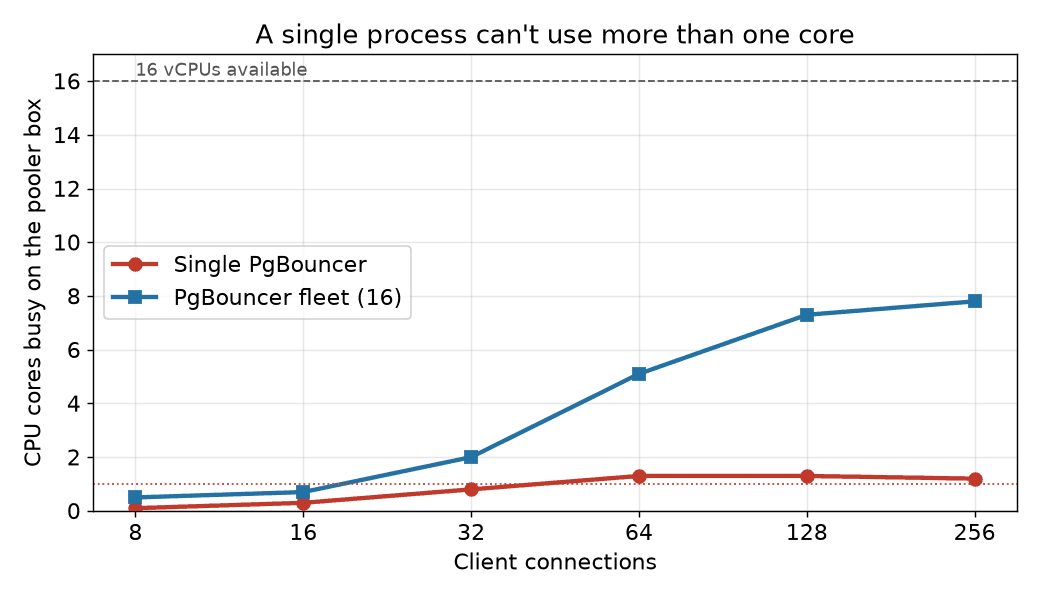
PgBouncer is single-threaded. A single process uses one CPU core, no matter how many the machine has. On a 16-vCPU box that means one core does all the connection pooling while the other fifteen sit idle, and the pooler starts capping throughput long before Postgres runs out of room.

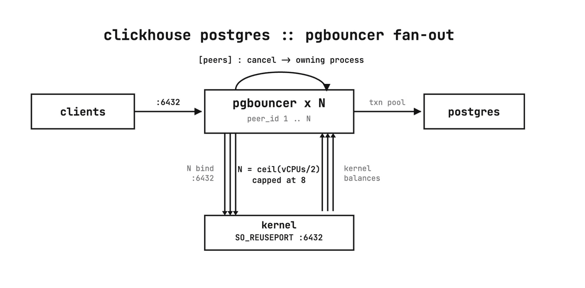
In ClickHouse Managed Postgres we run a fleet of PgBouncer processes, sized proportional to the available cores.

Every process in the fleet binds the same port with so_reuseport enabled. The kernel load-balances incoming connections across the processes, so clients still connect to a single endpoint and never know there is more than one PgBouncer behind it. This is the mechanism PgBouncer's own docs point to for using more than one core: it is single-threaded per process, and so_reuseport is how you put every core to work.

pgbouncer_jul2026_image5.png

The catch: query cancellation #

A Postgres cancel request arrives on a brand-new connection carrying a cancel key, separate from the connection running the query. With so_reuseport, the kernel is free to hand that new connection to a different process than the one holding the session. The cancel lands on a process that has never heard of the query, and nothing happens.

Peering fixes this. The processes are aware of one another, so a cancel that lands on the wrong process is forwarded to the one that actually owns the session. Cancellation works across the whole fleet, even though any given request can arrive anywhere.

Pooling runs in transaction mode, so a server connection is returned to the pool the moment a transaction commits. And the connection budget is split across the fleet: max_client_conn and max_db_connections are divided by the number of processes, so the fleet as a whole never oversubscribes Postgres.

Seeing it on real hardware #

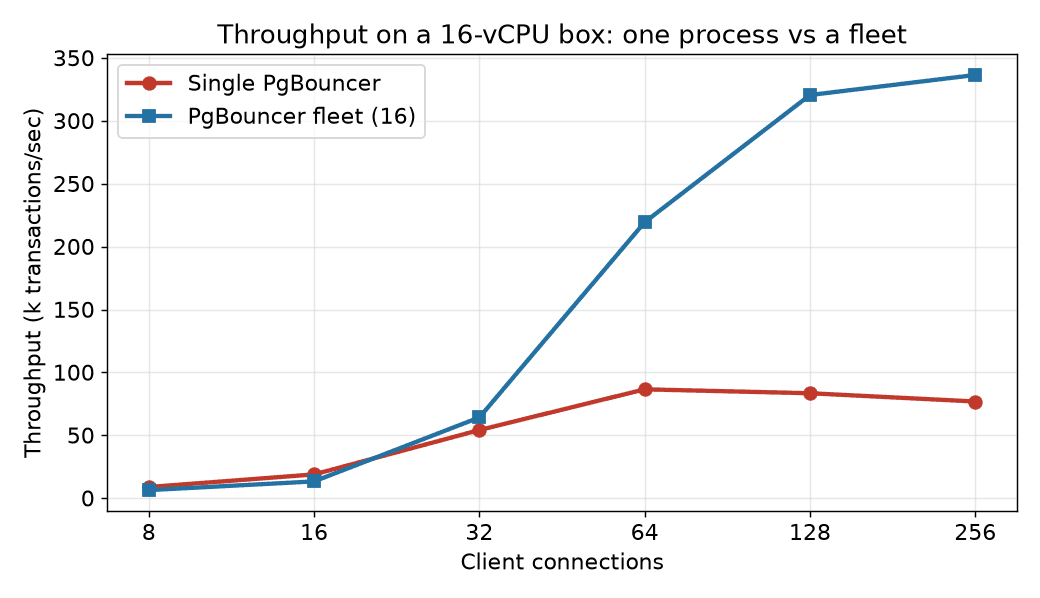
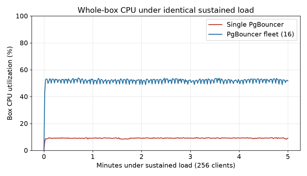
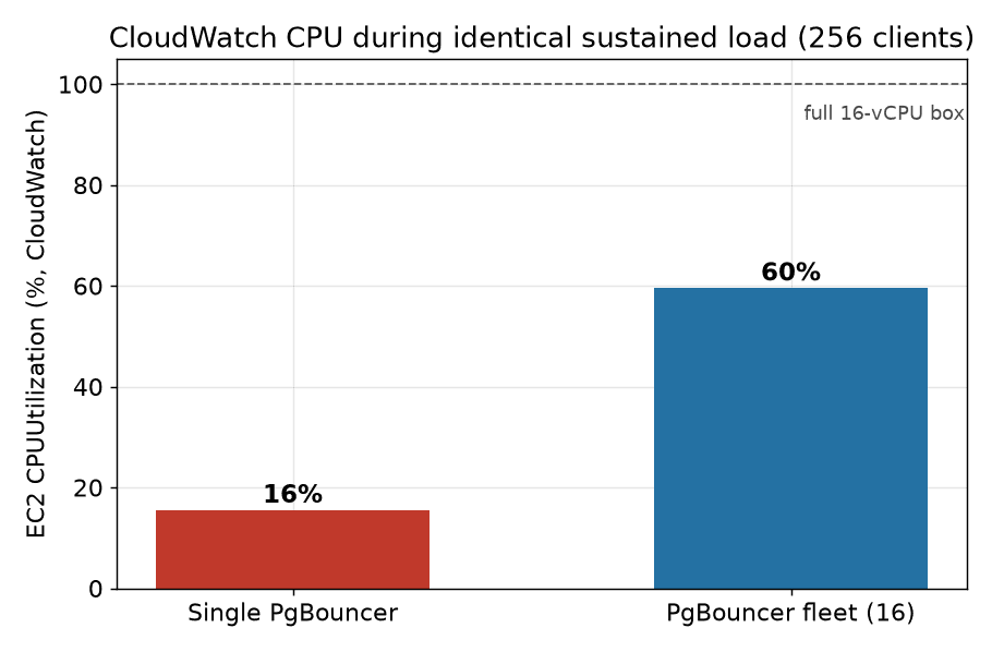
We ran both configurations on identical AWS EC2 instances: a 16-vCPU c7i.4xlarge for the pooler, a separate box for Postgres, and a third driving load with pgbench in select-only, transaction-pooled mode. One pooler box ran a single PgBouncer process; the other ran a fleet of 16. Same instance type, same Postgres, same workload. The only variable is one process versus sixteen.

We ramped client connections from 8 to 256 and measured throughput and how much of the 16-core box each pooler actually used.

The single process peaks around 87k transactions/sec and then gets worse under more load, sliding to 77k at 256 clients as everything contends for one core. The fleet keeps climbing to roughly 336k transactions/sec, about 4x, because it has more cores to climb into.

The single process never gets past about one core of work: under load, pidstat shows the PgBouncer process pinned at ~97% CPU, a full core, while the 16-vCPU box as a whole stays under 10% utilized. The fleet spreads across the machine, reaching roughly 8 cores busy, and it still had headroom when Postgres and the load generator became the limit.

Hold 256 clients steady against each box: the single-process box runs near 9% CPU for the entire run while the fleet holds around 52%. Same instance type, same Postgres, same workload. One configuration leaves the machine idle, the other puts it to work.

EC2's own CloudWatch metric says the same thing from outside the guest: during the load the single-process instance averages about 16% CPUUtilization, the fleet about 60%. CloudWatch reads a little higher than the in-guest number, but the same gap holds: on a box you're paying 16 vCPUs for, a single PgBouncer leaves almost all of it on the floor.

The connection ceiling behaves the same way. A single process enforces max_client_conn on its own, and once you cross it, new clients are turned away:

1FATAL:  no more connections allowed (max_client_conn)

Splitting the budget across the fleet is what lets you raise the aggregate ceiling while keeping each process, and Postgres, within safe limits.

ClientsSingle TPSSingle box CPUFleet TPSFleet box CPU88,9100.8%6,4502.9%3254,2035.2%64,24412.3%6486,5708.3%219,43931.9%12883,4638.1%320,54745.9%25676,8937.7%336,46948.9%

At a handful of connections the single process is actually fine, even a hair faster, since there's nothing to parallelize and the fleet's connections are spread thin. The gap opens exactly where it matters: under real concurrency, where one core becomes the wall.

The takeaway #

A single PgBouncer is a fine default until the pooler, not Postgres, is what caps your throughput. Sizing a fleet to the cores, sharing one port with so_reuseport, and wiring the processes together with peering turns the pooler back into plumbing instead of a bottleneck.

Every ClickHouse Managed Postgres server ships with this setup by default. Provision a Postgres and see it in action.

The Daily Front Page 9 of 25
Saturday, July 11, 2026 The Daily Front No. 2 — SQLite With a Spine
article

Prefer strict tables in SQLite

by ingve·▲ 330 points·165 comments·evanhahn.com ↗
“Strict tables help enforce rigid typing, preventing mistakes like putting text into integer columns.”

In short: I prefer strict tables in SQLite because they avoid some datatype problems, such as putting text in number columns.

SQLite has a feature that I think is underrated: strict tables. Strict tables help enforce rigid typing, preventing mistakes like putting text into integer columns. I like them, and wrote this post to promote their use!

To make a strict table, add STRICT to the end of its definition. Like this:

-CREATE TABLE people (name TEXT);
+CREATE TABLE people (name TEXT) STRICT;

That’s it! But what does it do?

Advantages of strict tables

Broadly, strict tables help enforce rigid types, like other SQL engines do.

Prevents type mismatches on insert/update

Most significantly, strict tables keep you from inserting the wrong type into a column. For example, SQLite normally lets you put text into an INTEGER column, but not with strict tables.

-- Non-strict tables let you put anything anywhere.
CREATE TABLE people_nonstrict (age INTEGER);
INSERT INTO people_nonstrict (age) VALUES ('garbage');
-- => works fine

-- Strict tables don't allow that, which I prefer.
CREATE TABLE people_strict (age INTEGER) STRICT;
INSERT INTO people_strict (age) VALUES ('garbage');
-- => error: cannot store TEXT value in INTEGER column

Personally, I think it’s a mistake to try to put text in an integer column, or vice-versa. I don’t want SQLite to let me make this error!

The same validation happens for UPDATEs, too.

Notably, if a value can be losslessly converted, it will still be accepted. For example, the string '123' can be perfectly converted to an integer, so it’s allowed. These two lines are equivalent, even for a strict table:

INSERT INTO people_strict (age) VALUES ('123');
INSERT INTO people_strict (age) VALUES (123);

Prevents bogus column types on table creation

By default, you can create columns with bogus types. For example, all of these work even though they aren’t valid SQLite datatypes:

-- SQLite doesn't support these types, but this is all accepted.
CREATE TABLE tbl (name GARBAGE);
CREATE TABLE tbl (name DATETIME);
CREATE TABLE tbl (name JSON);
CREATE TABLE tbl (name UUID);
CREATE TABLE tbl (name BLOBB);

I think these aren’t what the developer intended. Some of these are typos, some of them are misunderstandings of which datatypes SQLite supports, and some are egregious mistakes.

Appending STRICT to any of these statements makes them error. In my opinion, that’s the correct behavior!

-- All of these give errors, which I prefer.
CREATE TABLE tbl (name GARBAGE) STRICT;
CREATE TABLE tbl (name DATETIME) STRICT;
CREATE TABLE tbl (name JSON) STRICT;
CREATE TABLE tbl (name UUID) STRICT;
CREATE TABLE tbl (name BLOBB) STRICT;

Only INT, INTEGER, REAL, TEXT, BLOB, and ANY are allowed.

Strict tables also require a column type, so you can’t do CREATE TABLE tbl (name).

Still allows flexibility with ANY

If you still need a column to be flexible, you can use the ANY datatype. As the name suggests, it allows anything—even in a strict table.

CREATE TABLE tbl (value ANY) STRICT;

-- All of these are valid because the column is ANY:
INSERT INTO tbl (value) VALUES (123);
INSERT INTO tbl (value) VALUES ('text');
INSERT INTO tbl (value) VALUES (12.34);
INSERT INTO tbl (value) VALUES (X'8647');

I haven’t found a use for this, but maybe you will!

Disadvantages of strict tables

I prefer strict tables but I must share a few cons. Not everything is better!

Can’t strict-ify an existing table

I think it’s best to use strictness from the start, but that’s not always possible.

Unfortunately, I don’t think there’s a way to ALTER a table to make it strict. I think you have to copy the data out of the non-strict table into the strict one. Something like this:

-- 1. Create a new strict table with the same schema
CREATE TABLE new_people (name TEXT) STRICT;

-- 2. Copy data (risky if types are wrong!)
INSERT INTO new_people SELECT * FROM people;

-- 3. Replace the old table
DROP TABLE people;
ALTER TABLE new_people RENAME TO people;

Note that this could be tricky if the non-strict table has invalid data! For example, if the old data accidentally contains text in an integer column, you’ll get errors when doing the migration. You’ll probably need to clean the data or cast it.

You could make a rule for your codebase that all new tables are strict. That might be useful—at least some of your tables are valid! But it might also mean you have inconsistent validation across your tables, which might be more surprising than having weak validation on all tables. It’s up to you to decide whether this is a good fit for you.

The SQLite developers disagree with me

SQLite has a whole page called “The Advantages Of Flexible Typing”, where they argue that SQLite’s flexible behavior is good, actually.

I hesitate to wade into the controversy of static-versus-dynamic, but I disagree in most cases. I’ve personally encountered many bugs where an unexpected data type caused subtle headaches. I’d much rather these mistakes explode loudly. But it’s worth noting that SQLite’s developers seem not to share my preference for strict tables!

They point out a few good uses for flexible tables, such as “a pure key-value store” or “a place to store miscellaneous attributes” of different types. They also mention that you might want to keep the invalid data in some cases, like if you’re directly importing a messy CSV and don’t want to lose any data. I still prefer strict tables, but acknowledge there are some reasonable cases for non-strict ones.

(There’s also at least one comment in the SQLite source that calls non-strict tables “legacy”, but I trust that less than the official documentation.)

Only in SQLite 3.37.0+

SQLite introduced strict tables in version 3.37.0, released November 2021. If you’re on an older version of SQLite, you can’t use strict tables.

It’s worth noting that old versions of SQLite can’t read databases with strict tables. For example, if you create a strict table in the newest version of SQLite and then try to read that database in SQLite 3.36.0 (before strict tables were added), you’ll get an error—even if the strict table is already in the database.

Performance maybe?

Strict tables are theoretically slower because they have to do a little extra work. For example, they check datatypes when doing an insert or update.

But in practice, I don’t think this is an issue. I wrote a hacky script that inserted millions of rows into a table with 100 columns, and there was no obvious difference on multiple machines I tried. The file size on disk was also the same. I didn’t test this thoroughly, so maybe there’s something I missed, but I don’t think strict tables present a performance problem.

In fact, one might expect better performance because you won’t be accidentally mismatching SQLite’s column affinities. But again, I haven’t tested this.

Conclusion: I like strict tables!

Personally, I think the pros of strict tables outweigh the cons.

I generally prefer when types are rigidly enforced. It squashes a class of mistakes, and help enforce good data integrity. They’re not a panacea, but they’re usually easy to add and go a long way.

If there’s a SQLite feature you think is underrated, please tell me.

The Daily Front Page 10 of 25
Saturday, July 11, 2026 The Daily Front No. 2 — Files Atop Buckets
article

ZeroFS vs. Amazon S3 Files

by cbrewster·▲ 88 points·29 comments·zerofs.net ↗
“Amazon S3 Files and ZeroFS expose POSIX filesystems backed by object storage, but the shared interface hides opposite bucket layouts.”

Amazon S3 Files and ZeroFS expose POSIX filesystems backed by object storage, but the shared interface hides opposite bucket layouts. The choice turns on the role of the bucket: if files must remain ordinary S3 objects, S3 Files preserves that identity; if the bucket can be an internal persistence layer, ZeroFS trades direct S3 access for packing, compression, and client-side encryption.

Storage layout

The defining property of S3 Files, which is built using Amazon EFS, is that images/cat.jpg on the mount corresponds to the same key in the bucket, with changes flowing in both directions. Active data and metadata reside in a low-latency tier that AWS calls “high-performance storage.”

That one-file, one-object identity is deliberately absent from the ZeroFS storage format. Metadata lives in an LSM tree; file contents are split into extents, compressed and encrypted, then packed into immutable segment objects. An S3 client sees an opaque internal layout rather than the mounted files.

flowchart TB
    subgraph CLIENTS["Client Layer"]
        NFS["NFS Client"]
        P9["9P Client"]
        NBD["NBD Client"]
        WEB["Web Browser"]
    end
    subgraph CORE["ZeroFS Core"]
        NFSD["NFS Server"]
        P9D["9P Server"]
        NBDD["NBD Server"]
        WEBUI["Web UI"]
        VFS["Virtual Filesystem"]
        SEG["Segment store: compressed, encrypted file-data frames"]
        SLATE["LSM tree: metadata and 32-byte extent pointers"]
        CACHE["Local Cache"]
        NFSD --> VFS
        P9D --> VFS
        NBDD --> VFS
        WEBUI --> VFS
        VFS --> SEG
        VFS --> SLATE
        SEG --> CACHE
        SLATE --> CACHE
    end
    subgraph BACKEND["Storage Backend"]
        SEGOBJ["Immutable segment objects"]
        SSTS["Metadata SSTs and manifest"]
        S3["S3 Object Store"]
        CACHE --> SEGOBJ
        CACHE --> SSTS
        SEGOBJ --> S3
        SSTS --> S3
    end
    NFS --> NFSD
    P9 --> P9D
    NBD --> NBDD
    WEB --> WEBUI
  

ZeroFS keeps file data and filesystem metadata on separate paths until both reach the object store.

Both mounts use the client page cache. The write-path row below starts after the client sends the write to the server.

Amazon S3 FilesZeroFS Storage modelAWS-managed high-performance storage synchronized with a bucket; internal layout not documentedAn LSM tree and immutable data segments on object storage Object layoutOne file maps to one S3 objectMetadata in an LSM tree; file-data frames packed into segments Write path after client cacheNFS write to high-performance storage, durable immediately; asynchronous S3 export after write inactivityOver 9P, fsync uploads data segments and flushes LSM metadata to object storage before returning success Cold read and read-aheadLinux NFS read-ahead, directory metadata import, optional small-file import, or direct S3 readLSM lookup, then adaptive object and cross-segment frame prefetch S3 API access to filesYes; filesystem changes appear after asynchronous exportNo; reading files requires ZeroFS and the encryption password Client interfaceNFS 4.1/4.29P or NFS for files; NBD for blocks Object-store choiceAmazon S3Amazon S3, S3-compatible stores, Azure Blob, or Google Cloud Storage Cost modelS3 plus high-performance storage, file access, and synchronization chargesObject storage and requests, plus the compute and cache running ZeroFS

Object interoperability

Keeping that one-to-one mapping means a file written through the mount eventually becomes a normal S3 object. Export begins after 60 seconds without a write, so continued writes postpone S3 visibility. Once export completes, existing tools can read the object with GetObject, and S3-side changes flow back into the filesystem. If both sides modify the same file before synchronization, S3 wins and the file-side version moves to lost+found.

A ZeroFS pathname cannot be fetched with the S3 API, and a segment cannot be scanned as Parquet. In exchange, small files need neither one data object nor one PUT each: their extents are compressed, encrypted, and packed together. The bucket and raw local cache contain ciphertext, so mounting or recovery requires ZeroFS and its encryption password. The encryption documentation lists the structural metadata that remains visible.

If other applications need immediate S3 visibility after a filesystem write, neither model provides it: S3 Files exports asynchronously, while ZeroFS never exposes mounted files through the S3 API.

Cold access

The first S3 Files access can trigger an import: listing a directory loads every object's metadata and asynchronously copies files below the import threshold, 128 KiB by default, into high-performance storage. AWS says a first listing of 1,000 objects may take several seconds. Larger files stay in S3, and reads of at least 1 MiB go directly to S3.

ZeroFS instead populates a local RAM and disk cache from reads and uploads. Newly sealed segments enter the cache from bytes already in hand, so read-after-write needs no GET; the cache is not write-back, and writes still reach object storage when segments are sealed and metadata is flushed. A cold miss resolves the requested extents through the LSM tree and coalesces adjacent frames into ranged GETs. It pays the first object-store round trip without importing the rest of the file or every small file in the directory; once the working set fits locally, data reads generate few S3 requests.

Both paths add read-ahead for sequential traffic: ZeroFS prefetches within and across segment objects, while S3 Files relies on Linux NFS read-ahead alongside its direct-S3 routing.

Cost

S3 storage and request charges apply in either case. S3 Files also charges for its high-performance storage tier: resident storage per GB-month and reads and writes per GB. The AWS pricing example current at publication uses these rates:

S3 Files chargeRate used in AWS's exampleWhen it applies High-performance storage$0.30 per GB-monthFiles have a 10 KiB minimum billable size File reads$0.03 per GBReads from high-performance storage, including exports to S3 File writes$0.06 per GBWrites to high-performance storage, including imports from S3

The amount resident in high-performance storage depends on the configured import threshold and expiration window. Listing imports metadata and eligible small files, reads can load more data, and file metadata does not expire. Imports are metered as filesystem writes and exports as reads; the minimum operation sizes are 32 KiB for file data and 4 KiB for metadata. AWS reports resident bytes and inodes in CloudWatch, but total bucket size alone cannot forecast the bill.

Illustrative model: store 10,000 GiB and read it once

This is an illustrative scenario, not a general cost comparison. It uses 10,000 AWS billable GB (GiB) of logical data in S3 Standard in us-east-1, at $0.023 per GB-month. The direct case assumes 1 MiB reads from data already in S3; the resident case assumes reads below 1 MiB with all data also in high-performance storage. Internet egress is excluded.

CaseStorage/monthRead onceIllustrative subtotal ZeroFS (2:1)$115 + overheadS3 GETs$115 + infrastructure ZeroFS (1:1)$230 + overheadS3 GETs$230 + infrastructure S3 Files (1 MiB direct reads)$230 + metadata$1.17 + S3 GETs~$231 + metadata and requests S3 Files (small resident reads)$3,230$300$3,530
+$600 if imported

The ZeroFS figures are estimates: compression reduces payload bytes, while metadata, temporary compaction data, and requests add cost. At an ideal 8 MiB GET size, reading the file data costs about $0.26 at 2:1 compression or $0.51 at 1:1, before metadata and short or random reads. ZeroFS also requires one server, or two for high availability, plus local disk cache; each node needs about 2 GB of RAM beyond its configured memory cache. S3 Files may therefore cost less for large-file streaming. The difference grows when data is imported into, or written through, high-performance storage: writing 10,000 GiB through S3 Files adds $600 in filesystem writes and $300 for export, while a month of residency adds $3,000.

Actual costs depend on file count, compression, I/O size, residency, fsync frequency, and infrastructure. S3 Files also requires bucket versioning, so noncurrent versions need an appropriate lifecycle rule.

fsync and S3 visibility

Durability and S3 visibility are separate events in S3 Files. Writes to high-performance storage are durable immediately, but export starts only after approximately 60 seconds without a write; calling fsync does not make the object immediately visible through the S3 API. ZeroFS has no second visibility event because there is no export step. Over 9P, a successful fsync returns after object storage acknowledges the data segment and its LSM metadata, leaving the file recoverable after a cold restart.

Rename

S3 has no directories or atomic rename for general-purpose buckets. S3 Files renames on the mount, then copies each affected object to a new key and deletes the old one; during a directory rename, both prefixes can be visible. AWS says synchronizing 100,000 renamed files takes a few minutes. ZeroFS changes only its LSM directory entries, with no copy per descendant and no S3 prefix exposed to object clients.


The mount points may look similar, but the buckets make different promises: S3 Files preserves ordinary objects for the surrounding S3 ecosystem; ZeroFS treats object storage as the private substrate of the filesystem.

The Daily Front Page 11 of 25
Saturday, July 11, 2026 The Daily Front No. 2 — Memory, Interrupted
article

Preemption is GC for memory reordering (2019)

by mpweiher·▲ 49 points·7 comments·pvk.ca ↗
“Preemption ought to be treated as a sunk cost, like garbage collection: we’re already paying for it, so we might as well use it.”

I previously noted how preemption makes lock-free programming harder in userspace than in the kernel. I now believe that preemption ought to be treated as a sunk cost, like garbage collection: we’re already paying for it, so we might as well use it. Interrupt processing (returning from an interrupt handler, actually) is fully serialising on x86, and on other platforms, no doubt: any userspace instruction either fully executes before the interrupt, or is (re-)executed from scratch some time after the return back to userspace. That’s something we can abuse to guarantee ordering between memory accesses, without explicit barriers.

This abuse of interrupts is complementary to Bounded TSO. Bounded TSO measures the hardware limit on the number of store instructions that may concurrently be in-flight (and combines that with the knowledge that instructions are retired in order) to guarantee liveness without explicit barriers, with no overhead, and usually marginal latency. However, without worst-case execution time information, it’s hard to map instruction counts to real time. Tracking interrupts lets us determine when enough real time has elapsed that earlier writes have definitely retired, albeit after a more conservative delay than Bounded TSO’s typical case.

I reached this position after working on two lock-free synchronisation primitives—event counts, and asymmetric flag flips as used in hazard pointers and epoch reclamation—that are similar in that a slow path waits for a sign of life from a fast path, but differ in the way they handle “stuck” fast paths. I’ll cover the event count and flag flip implementations that I came to on Linux/x86[-64], which both rely on interrupts for ordering. Hopefully that will convince you too that preemption is a useful source of pre-paid barriers for lock-free code in userspace.

I’m writing this for readers who are already familiar with lock-free programming, safe memory reclamation techniques in particular, and have some experience reasoning with formal memory models. For more references, Samy’s overview in the ACM Queue is a good resource. I already committed the code for event counts in Concurrency Kit, and for interrupt-based reverse barriers in my barrierd project.

Event counts with x86-TSO and futexes

An event count is essentially a version counter that lets threads wait until the current version differs from an arbitrary prior version. A trivial “wait” implementation could spin on the version counter. However, the value of event counts is that they let lock-free code integrate with OS-level blocking: waiters can grab the event count’s current version v0, do what they want with the versioned data, and wait for new data by sleeping rather than burning cycles until the event count’s version differs from v0. The event count is a common synchronisation primitive that is often reinvented and goes by many names (e.g., blockpoints); what matters is that writers can update the version counter, and waiters can read the version, run arbitrary code, then efficiently wait while the version counter is still equal to that previous version.

The explicit version counter solves the lost wake-up issue associated with misused condition variables, as in the pseudocode below.

bad condition waiter:

while True:
    atomically read data
    if need to wait:
        WaitOnConditionVariable(cv)
    else:
        break

In order to work correctly, condition variables require waiters to acquire a mutex that protects both data and the condition variable, before checking that the wait condition still holds and then waiting on the condition variable.

good condition waiter:

while True:
    with(mutex):
        read data
        if need to wait:
	        WaitOnConditionVariable(cv, mutex)
	    else:
	        break Waiters must prevent writers from making changes to the data, otherwise the data change (and associated condition variable wake-up) could occur between checking the wait condition, and starting to wait on the condition variable.  The waiter would then have missed a wake-up and could end up sleeping forever, waiting for something that has already happened.

good condition waker:

with(mutex):
    update data
    SignalConditionVariable(cv)

The six diagrams below show the possible interleavings between the signaler (writer) making changes to the data and waking waiters, and a waiter observing the data and entering the queue to wait for changes. The two left-most diagrams don’t interleave anything; these are the only scenarios allowed by correct locking. The remaining four actually interleave the waiter and signaler, and show that, while three are accidentally correct (lucky), there is one case, WSSW, where the waiter misses its wake-up.
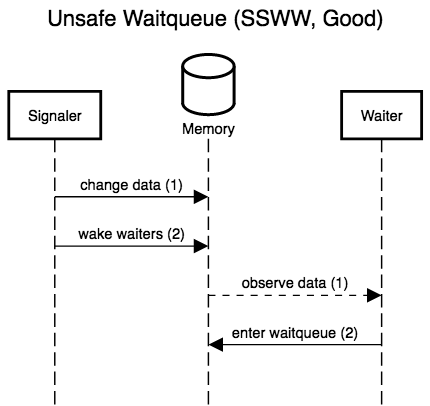
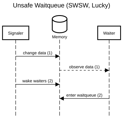
If any waiter can prevent writers from making progress, we don’t have a lock-free protocol. Event counts let waiters detect when they would have been woken up (the event count’s version counter has changed), and thus patch up this window where waiters can miss wake-ups for data changes they have yet to observe. Crucially, waiters detect lost wake-ups, rather than preventing them by locking writers out. Event counts thus preserve lock-freedom (and even wait-freedom!).

We could, for example, use an event count in a lock-free ring buffer: rather than making consumers spin on the write pointer, the write pointer could be encoded in an event count, and consumers would then efficiently block on that, without burning CPU cycles to wait for new messages.

The challenging part about implementing event counts isn’t making sure to wake up sleepers, but to only do so when there are sleepers to wake. For some use cases, we don’t need to do any active wake-up, because exponential backoff is good enough: if version updates signal the arrival of a response in a request/response communication pattern, exponential backoff, e.g., with a 1.1x backoff factor, could bound the increase in response latency caused by the blind sleep during backoff, e.g., to 10%.

Unfortunately, that’s not always applicable. In general, we can’t assume that signals corresponds to responses for prior requests, and we must support the case where progress is usually fast enough that waiters only spin for a short while before grabbing more work. The latter expectation means we can’t “just” unconditionally execute a syscall to wake up sleepers whenever we increment the version counter: that would be too slow. This problem isn’t new, and has a solution similar to the one deployed in adaptive spin locks.

The solution pattern for adaptive locks relies on tight integration with an OS primitive, e.g., futexes. The control word, the machine word on which waiters spin, encodes its usual data (in our case, a version counter), as well as a new flag to denote that there are sleepers waiting to be woken up with an OS syscall. Every write to the control word uses atomic read-modify-write instructions, and before sleeping, waiters ensure the “sleepers are present” flag is set, then make a syscall to sleep only if the control word is still what they expect, with the sleepers flag set.

OpenBSD’s compatibility shim for Linux’s futexes is about as simple an implementation of the futex calls as it gets. The OS code for futex wake and wait is identical to what userspace would do with mutexes and condition variables (waitqueues). Waiters lock out wakers for the futex word or a coarser superset, check that the futex word’s value is as expected, and enters the futex’s waitqueue. Wakers acquire the futex word for writes, and wake up the waitqueue. The difference is that all of this happens in the kernel, which, unlike userspace, can force the scheduler to be helpful. Futex code can run in the kernel because, unlike arbitrary mutex/condition variable pairs, the protected data is always a single machine integer, and the wait condition an equality test. This setup is simple enough to fully implement in the kernel, yet general enough to be useful.

OS-assisted conditional blocking is straightforward enough to adapt to event counts. The control word is the event count’s version counter, with one bit stolen for the “sleepers are present” flag (sleepers flag).

Incrementing the version counter can use a regular atomic increment; we only need to make sure we can tell whether the sleepers flag might have been set before the increment. If the sleepers flag was set, we clear it (with an atomic bit reset), and wake up any OS thread blocked on the control word.

increment event count:

old <- fetch_and_add(event_count.counter, 2)  # flag is in the low bit
if (old & 1):
    atomic_and(event_count.counter, -2)
    signal waiters on event_count.counter

Waiters can spin for a while, waiting for the version counter to change. At some point, a waiter determines that it’s time to stop wasting CPU time. The waiter then sets the sleepers flag with a compare-and-swap: the CAS (compare-and-swap) can only fail because the counter’s value has changed or because the flag is already set. In the former failure case, it’s finally time to stop waiting. In the latter failure care, or if the CAS succeeded, the flag is now set. The waiter can then make a syscall to block on the control word, but only if the control word still has the sleepers flag set and contains the same expected (old) version counter.

wait until event count differs from prev:

repeat k times:
    if (event_count.counter / 2) != prev:  # flag is in low bit.
        return
compare_and_swap(event_count.counter, prev * 2, prev * 2 + 1)
if cas_failed and cas_old_value != (prev * 2 + 1):
    return
repeat k times:
    if (event_count.counter / 2) != prev:
        return
sleep_if(event_count.center == prev * 2 + 1)

This scheme works, and offers decent performance. In fact, it’s good enough for Facebook’s Folly.
I certainly don’t see how we can improve on that if there are concurrent writers (incrementing threads).

However, if we go back to the ring buffer example, there is often only one writer per ring. Enqueueing an item in a single-producer ring buffer incurs no atomic, only a release store: the write pointer increment only has to be visible after the data write, which is always the case under the TSO memory model (including x86). Replacing the write pointer in a single-producer ring buffer with an event count where each increment incurs an atomic operation is far from a no-brainer. Can we do better, when there is only one incrementer?

On x86 (or any of the zero other architectures with non-atomic read-modify-write instructions and TSO), we can… but we must accept some weirdness.

The operation that must really be fast is incrementing the event counter, especially when the sleepers flag is not set. Setting the sleepers flag on the other hand, may be slower and use atomic instructions, since it only happens when the executing thread is waiting for fresh data.

I suggest that we perform the former, the increment on the fast path, with a non-atomic read-modify-write instruction, either inc mem or xadd mem, reg. If the sleepers flag is in the sign bit, we can detect it (modulo a false positive on wrap-around) in the condition codes computed by inc; otherwise, we must use xadd (fetch-and-add) and look at the flag bit in the fetched value.

The usual ordering-based arguments are no help in this kind of asymmetric synchronisation pattern. Instead, we must go directly to the x86-TSO memory model. All atomic (LOCK prefixed) instructions conceptually flush the executing core’s store buffer, grab an exclusive lock on memory, and perform the read-modify-write operation with that lock held. Thus, manipulating the sleepers flag can’t lose updates that are already visible in memory, or on their way from the store buffer. The RMW increment will also always see the latest version update (either in global memory, or in the only incrementer’s store buffer), so won’t lose version updates either. Finally, scheduling and thread migration must always guarantee that the incrementer thread sees its own writes, so that won’t lose version updates.

increment event count without atomics in the common case:

old <- non_atomic_fetch_and_add(event_count.counter, 2)
if (old & 1):
    atomic_and(event_count.counter, -2)
    signal waiters on event_count.counter

The only thing that might be silently overwritten is the sleepers flag: a waiter might set that flag in memory just after the increment’s load from memory, or while the increment reads a value with the flag unset from the local store buffer. The question is then how long waiters must spin before either observing an increment, or knowing that the flag flip will be observed by the next increment. That question can’t be answered with the memory model, and worst-case execution time bounds are a joke on contemporary x86.

I found an answer by remembering that IRET, the instruction used to return from interrupt handlers, is a full barrier.1 We also know that interrupts happen at frequent and regular intervals, if only for the preemption timer (every 4-10ms on stock Linux/x86oid).

Regardless of the bound on store visibility, a waiter can flip the sleepers-are-present flag, spin on the control word for a while, and then start sleeping for short amounts of time (e.g., a millisecond or two at first, then 10 ms, etc.): the spin time is long enough in the vast majority of cases, but could still, very rarely, be too short.

At some point, we’d like to know for sure that, since we have yet to observe a silent overwrite of the sleepers flag or any activity on the counter, the flag will always be observed and it is now safe to sleep forever. Again, I don’t think x86 offers any strict bound on this sort of thing. However, one second seems reasonable. Even if a core could stall for that long, interrupts fire on every core several times a second, and returning from interrupt handlers acts as a full barrier. No write can remain in the store buffer across interrupts, interrupts that occur at least once per second. It seems safe to assume that, once no activity has been observed on the event count for one second, the sleepers flag will be visible to the next increment.

That assumption is only safe if interrupts do fire at regular intervals. Some latency sensitive systems dedicate cores to specific userspace threads, and move all interrupt processing and preemption away from those cores. A correctly isolated core running Linux in tickless mode, with a single runnable process, might not process interrupts frequently enough. However, this kind of configuration does not happen by accident. I expect that even a half-second stall in such a system would be treated as a system error, and hopefully trigger a watchdog. When we can’t count on interrupts to get us barriers for free, we can instead rely on practical performance requirements to enforce a hard bound on execution time.

Either way, waiters set the sleepers flag, but can’t rely on it being observed until, very conservatively, one second later. Until that time has passed, waiters spin on the control word, then block for short, but growing, amounts of time. Finally, if the control word (event count version and sleepers flag) has not changed in one second, we assume the incrementer has no write in flight, and will observe the sleepers flag; it is safe to block on the control word forever.

wait until event count differs from prev:

repeat k times:
    if (event_count.counter / 2) != prev:
        return
compare_and_swap(event_count.counter, 2 * prev, 2 * prev + 1)
if cas_failed and cas_old_value != 2 * prev + 1:
    return
repeat k times:
    if event_count.counter != 2 * prev + 1:
        return
repeat for 1 second:
    sleep_if_until(event_count.center == 2 * prev + 1,
                   $exponential_backoff)
    if event_count.counter != 2 * prev + 1:
        return
sleep_if(event_count.center == prev * 2 + 1)

That’s the solution I implemented in this pull request for SPMC and MPMC event counts in concurrency kit. The MP (multiple producer) implementation is the regular adaptive logic, and matches Folly’s strategy. It needs about 30 cycles for an uncontended increment with no waiter, and waking up sleepers adds another 700 cycles on my E5-46xx (Linux 4.16). The single producer implementation is identical for the slow path, but only takes ~8 cycles per increment with no waiter, and, eschewing atomic instruction, does not flush the pipeline (i.e., the out-of-order execution engine is free to maximise throughput). The additional overhead for an increment without waiter, compared to a regular ring buffer pointer update, is 3-4 cycles for a single predictable conditional branch or fused test and branch, and the RMW’s load instead of a regular add/store. That’s closer to zero overhead, which makes it much easier for coders to offer OS-assisted blocking in their lock-free algorithms, without agonising over the penalty when no one needs to block.

Asymmetric flag flip with interrupts on Linux

Hazard pointers and epoch reclamation. Two different memory reclamation technique, in which the fundamental complexity stems from nearly identical synchronisation requirements: rarely, a cold code path (which is allowed to be very slow) writes to memory, and must know when another, much hotter, code path is guaranteed to observe the slow path’s last write.

For hazard pointers, the cold code path waits until, having overwritten an object’s last persistent reference in memory, it is safe to destroy the pointee. The hot path is the reader:

1. read pointer value *(T **)x.
2. write pointer value to hazard pointer table
3. check that pointer value *(T **)x has not changed

Similarly, for epoch reclamation, a read-side section will grab the current epoch value, mark itself as reading in that epoch, then confirm that the epoch hasn’t become stale.

1. $epoch <- current epoch
2. publish self as entering a read-side section under $epoch
3. check that $epoch is still current, otherwise retry

Under a sequentially consistent (SC) memory model, the two sequences are valid with regular (atomic) loads and stores. The slow path can always make its write, then scan every other thread’s single-writer data to see if any thread has published something that proves it executed step 2 before the slow path’s store (i.e., by publishing the old pointer or epoch value).

The diagrams below show all possible interleavings. In all cases, once there is no evidence that a thread has failed to observe the slow path’s new write, we can correctly assume that all threads will observe the write. I simplified the diagrams by not interleaving the first read in step 1: its role is to provide a guess for the value that will be re-read in step 3, so, at least with respect to correctness, that initial read might as well be generating random values. I also kept the second “scan” step in the slow path abstract. In practice, it’s a non-snapshot read of all the epoch or hazard pointer tables for threads that execute the fast path: the slow path can assume an epoch or pointer will not be resurrected once the epoch or pointer is absent from the scan.

No one implements SC in hardware. X86 and SPARC offer the strongest practical memory model, Total Store Ordering, and that’s still not enough to correctly execute the read-side critical sections above without special annotations. Under TSO, reads (e.g., step 3) are allowed to execute before writes (e.g., step 2). X86-TSO models that as a buffer in which stores may be delayed, and that’s what the scenarios below show, with steps 2 and 3 of the fast path reversed (the slow path can always be instrumented to recover sequential order, it’s meant to be slow). The TSO interleavings only differ from the SC ones when the fast path’s steps 2 and 3 are separated by something on slow path’s: when the two steps are adjacent, their order relative to the slow path’s steps is unaffected by TSO’s delayed stores. TSO is so strong that we only have to fix one case, FSSF, where the slow path executes in the middle of the fast path, with the reversal of store and load order allowed by TSO.

Simple implementations plug this hole with a store-load barrier between the second and third steps, or implement the store with an atomic read-modify-write instruction that doubles as a barrier. Both modifications are safe and recover SC semantics, but incur a non-negligible overhead (the barrier forces the out of order execution engine to flush before accepting more work) which is only necessary a minority of the time.

The pattern here is similar to the event count, where the slow path signals the fast path that the latter should do something different. However, where the slow path for event counts wants to wait forever if the fast path never makes progress, hazard pointer and epoch reclamation must detect that case and ignore sleeping threads (that are not in the middle of a read-side SMR critical section).

In this kind of asymmetric synchronisation pattern, we wish to move as much of the overhead to the slow (cold) path. Linux 4.3 gained the membarrier syscall for exactly this use case. The slow path can execute its write(s) before making a membarrier syscall. Once the syscall returns, any fast path write that has yet to be visible (hasn’t retired yet), along with every subsequent instruction in program order, started in a state where the slow path’s writes were visible. As the next diagram shows, this global barrier lets us rule out the one anomalous execution possible under TSO, without adding any special barrier to the fast path.

The problem with membarrier is that it comes in two flavours: slow, or not scalable. The initial, unexpedited, version waits for kernel RCU to run its callback, which, on my machine, takes anywhere between 25 and 50 milliseconds. The reason it’s so slow is that the condition for an RCU grace period to elapse are more demanding than a global barrier, and may even require multiple such barriers. For example, if we used the same scheme to nest epoch reclamation ten deep, the outermost reclaimer would be 1024 times slower than the innermost one. In reaction to this slowness, potential users of membarrier went back to triggering IPIs, e.g., by mprotecting a dummy page. mprotect isn’t guaranteed to act as a barrier, and does not do so on AArch64, so Linux 4.16 added an “expedited” mode to membarrier. In that expedited mode, each membarrier syscall sends an IPI to every other core… when I look at machines with hundreds of cores, \(n - 1\) IPI per core, a couple times per second on every \(n\) core, start to sound like a bad idea.

Let’s go back to the observation we made for event count: any interrupt acts as a barrier for us, in that any instruction that retires after the interrupt must observe writes made before the interrupt. Once the hazard pointer slow path has overwritten a pointer, or the epoch slow path advanced the current epoch, we can simply look at the current time, and wait until an interrupt has been handled at a later time on all cores. The slow path can then scan all the fast path state for evidence that they are still using the overwritten pointer or the previous epoch: any fast path that has not published that fact before the interrupt will eventually execute the second and third steps after the interrupt, and that last step will notice the slow path’s update.

There’s a lot of information in /proc that lets us conservatively determine when a new interrupt has been handled on every core. However, it’s either too granular (/proc/stat) or extremely slow to generate (/proc/schedstat). More importantly, even with ftrace, we can’t easily ask to be woken up when something interesting happens, and are forced to poll files for updates (never mind the weirdly hard to productionalise kernel interface).

What we need is a way to read, for each core, the last time it was definitely processing an interrupt. Ideally, we could also block and let the OS wake up our waiter on changes to the oldest “last interrupt” timestamp, across all cores. On x86, that’s enough to get us the asymmetric barriers we need for hazard pointers and epoch reclamation, even if only IRET is serialising, and not interrupt handler entry. Once a core’s update to its “last interrupt” timestamp is visible, any write prior to the update, and thus any write prior to the interrupt is also globally visible: we can only observe the timestamp update from a different core than the updater, in which case TSO saves us, or after the handler has returned with a serialising IRET.

We can bundle all that logic in a short eBPF program.2 The program has a map of thread-local arrays (of 1 CLOCK_MONOTONIC timestamp each), a map of perf event queues (one per CPU), and an array of 1 “watermark” timestamp. Whenever the program runs, it gets the current time. That time will go in the thread-local array of interrupt timestamps. Before storing a new value in that array, the program first reads the previous interrupt time: if that time is less than or equal to the watermark, we should wake up userspace by enqueueing in event in perf. The enqueueing is conditional because perf has more overhead than a thread-local array, and because we want to minimise spurious wake-ups. A high signal-to-noise ratio lets userspace set up the read end of the perf queue to wake up on every event and thus minimise update latency.

We now need a single global daemon to attach the eBPF program to an arbitrary set of software tracepoints triggered by interrupts (or PMU events that trigger interrupts), to hook the perf fds to epoll, and to re-read the map of interrupt timestamps whenever epoll detects a new perf event. That’s what the rest of the code handles: setting up tracepoints, attaching the eBPF program, convincing perf to wake us up, and hooking it all up to epoll. On my fully loaded 24-core E5-46xx running Linux 4.18 with security patches, the daemon uses ~1-2% (much less on 4.16) of a core to read the map of timestamps every time it’s woken up every ~4 milliseconds. perf shows the non-JITted eBPF program itself uses ~0.1-0.2% of every core.

Amusingly enough, while eBPF offers maps that are safe for concurrent access in eBPF programs, the same maps come with no guarantee when accessed from userspace, via the syscall interface. However, the implementation uses a hand-rolled long-by-long copy loop, and, on x86-64, our data all fit in longs. I’ll hope that the kernel’s compilation flags (e.g., -ffree-standing) suffice to prevent GCC from recognising memcpy or memmove, and that we thus get atomic store and loads on x86-64. Given the quality of eBPF documentation, I’ll bet that this implementation accident is actually part of the API. Every BPF map is single writer (either per-CPU in the kernel, or single-threaded in userspace), so this should work.

Once the barrierd daemon is running, any program can mmap its data file to find out the last time we definitely know each core had interrupted userspace, without making any further syscall or incurring any IPI. We can also use regular synchronisation to let the daemon wake up threads waiting for interrupts as soon as the oldest interrupt timestamp is updated. Applications don’t even need to call clock_gettime to get the current time: the daemon also works in terms of a virtual time that it updates in the mmaped data file.

The barrierd data file also includes an array of per-CPU structs with each core’s timestamps (both from CLOCK_MONOTONIC and in virtual time). A client that knows it will only execute on a subset of CPUs, e.g., cores 2-6, can compute its own “last interrupt” timestamp by only looking at entries 2 to 6 in the array. The daemon even wakes up any futex waiter on the per-CPU values whenever they change. The convenience interface is pessimistic, and assumes that client code might run on every configured core. However, anyone can mmap the same file and implement tighter logic.

Again, there’s a snag with tickless kernels. In the default configuration already, a fully idle core might not process timer interrupts. The barrierd daemon detects when a core is falling behind, and starts looking for changes to /proc/stat. This backup path is slower and coarser grained, but always works with idle cores. More generally, the daemon might be running on a system with dedicated cores. I thought about causing interrupts by re-affining RT threads, but that seems counterproductive. Instead, I think the right approach is for users of barrierd to treat dedicated cores specially. Dedicated threads can’t (shouldn’t) be interrupted, so they can regularly increment a watchdog counter with a serialising instruction. Waiters will quickly observe a change in the counters for dedicated threads, and may use barrierd to wait for barriers on preemptively shared cores. Maybe dedicated threads should be able to hook into barrierd and check-in from time to time. That would break the isolation between users of barrierd, but threads on dedicated cores are already in a privileged position.

I quickly compared the barrier latency on an unloaded 4-way E5-46xx running Linux 4.16, with a sample size of 20000 observations per method (I had to remove one outlier at 300ms). The synchronous methods mprotect (which abuses mprotect to send IPIs by removing and restoring permissions on a dummy page), or explicit IPI via expedited membarrier, are much faster than the other (unexpedited membarrier with kernel RCU, or barrierd that counts interrupts). We can zoom in on the IPI-based methods, and see that an expedited membarrier (IPI) is usually slightly faster than mprotect; IPI via expedited membarrier hits a worst-case of 0.041 ms, versus 0.046 for mprotect.

The performance of IPI-based barriers should be roughly independent of system load. However, we did observe a slowdown for expedited membarrier (between \(68.4-73.0\%\) of the time, \(p < 10\sp{-12}\) according to a binomial test3) on the same 4-way system, when all CPUs were running CPU-intensive code at low priority. In this second experiment, we have a sample size of one million observations for each method, and the worst case for IPI via expedited membarrier was 0.076 ms (0.041 ms on an unloaded system), compared to a more stable 0.047 ms for mprotect.

Now for non-IPI methods: they should be slower than methods that trigger synchronous IPIs, but hopefully have lower overhead and scale better, while offering usable latencies.

On an unloaded system, the interrupts that drive barrierd are less frequent, sometimes outright absent, so unexpedited membarrier achieves faster response times. We can even observe barrierd’s fallback logic, which scans /proc/stat for evidence of idle CPUs after 10 ms of inaction: that’s the spike at 20ms. The values for vtime show the additional slowdown we can expect if we wait on barrierd’s virtual time, rather than directly reading CLOCK_MONOTONIC. Overall, the worst case latencies for barrierd (53.7 ms) and membarrier (39.9 ms) aren’t that different, but I should add another fallback mechanism based on membarrier to improve barrierd’s performance on lightly loaded machines.

When the same 4-way, 24-core, system is under load, interrupts are fired much more frequently and reliably, so barrierd shines, but everything has a longer tail, simply because of preemption of the benchmark process. Out of the one million observations we have for each of unexpedited membarrier, barrierd, and barrierd with virtual time on this loaded system, I eliminated 54 values over 100 ms (18 for membarrier, 29 for barrierd, and 7 for virtual time). The rest is shown below. barrierd is consistently much faster than membarrier, with a geometric mean speedup of 23.8x. In fact, not only can we expect barrierd to finish before an unexpedited membarrier \(99.99\%\) of the time (\(p<10\sp{-12}\) according to a binomial test), but we can even expect barrierd to be 10 times as fast \(98.3-98.5\%\) of the time (\(p<10\sp{-12}\)). The gap is so wide that even the opportunistic virtual-time approach is faster than membarrier (geometric mean of 5.6x), but this time with a mere three 9s (as fast as membarrier \(99.91-99.96\%\) of the time, \(p<10\sp{-12}\)).

With barrierd, we get implicit barriers with worse overhead than unexpedited membarrier (which is essentially free since it piggybacks on kernel RCU, another sunk cost), but 1/10th the latency (0-4 ms instead of 25-50 ms). In addition, interrupt tracking is per-CPU, not per-thread, so it only has to happen in a global single-threaded daemon; the rest of userspace can obtain the information it needs without causing additional system overhead. More importantly, threads don’t have to block if they use barrierd to wait for a system-wide barrier. That’s useful when, e.g., a thread pool worker is waiting for a reverse barrier before sleeping on a futex. When that worker blocks in membarrier for 25ms or 50ms, there’s a potential hiccup where a work unit could sit in the worker’s queue for that amount of time before it gets processed. With barrierd (or the event count described earlier), the worker can spin and wait for work units to show up until enough time has passed to sleep on the futex.

While I believe that information about interrupt times should be made available without tracepoint hacks, I don’t know if a syscall like membarrier is really preferable to a shared daemon like barrierd. The one salient downside is that barrierd slows down when some CPUs are idle; that’s something we can fix by including a membarrier fallback, or by sacrificing power consumption and forcing kernel ticks, even for idle cores.

Preemption can be an asset

When we write lock-free code in userspace, we always have preemption in mind. In fact, the primary reason for lock-free code in userspace is to ensure consistent latency despite potentially adversarial scheduling. We spend so much effort to make our algorithms work despite interrupts and scheduling that we can fail to see how interrupts can help us. Obviously, there’s a cost to making our code preemption-safe, but preemption isn’t an option. Much like garbage collection in managed language, preemption is a feature we can’t turn off. Unlike GC, it’s not obvious how to make use of preemption in lock-free code, but this post shows it’s not impossible.

We can use preemption to get asymmetric barriers, nearly for free, with a daemon like barrierd. I see a duality between preemption-driven barriers and techniques like Bounded TSO: the former are relatively slow, but offer hard bounds, while the latter guarantee liveness, usually with negligible latency, but without any time bound.

I used preemption to make single-writer event counts faster (comparable to a regular non-atomic counter), and to provide a lower-latency alternative to membarrier’s asymmetric barrier. In a similar vein, SPeCK uses time bounds to ensure scalability, at the expense of a bit of latency, by enforcing periodic TLB reloads instead of relying on synchronous shootdowns. What else can we do with interrupts, timer or otherwise?

Thank you Samy, Gabe, and Hanes for discussions on an earlier draft. Thank you Ruchir for improving this final version.

P.S. event count without non-atomic RMW?

The single-producer event count specialisation relies on non-atomic read-modify-write instructions, which are hard to find outside x86. I think the flag flip pattern in epoch and hazard pointer reclamation shows that’s not the only option.

We need two control words, one for the version counter, and another for the sleepers flag. The version counter is only written by the incrementer, with regular non-atomic instructions, while the flag word is written to by multiple producers, always with atomic instructions.

The challenge is that OS blocking primitives like futex only let us conditionalise the sleep on a single word. We could try to pack a pair of 16-bit shorts in a 32-bit int, but that doesn’t give us a lot of room to avoid wrap-around. Otherwise, we can guarantee that the sleepers flag is only cleared immediately before incrementing the version counter. That suffices to let sleepers only conditionalise on the version counter… but we still need to trigger a wake-up if the sleepers flag was flipped between the last clearing and the increment.

On the increment side, the logic looks like

must_wake = false
if sleepers flag is set:
    must_wake = true
    clear sleepers flag
increment version
if must_wake or sleepers flag is set:
    wake up waiters

and, on the waiter side, we find

if version has changed
    return
set sleepers flag
sleep if version has not changed

The separate “sleepers flag” word doubles the space usage, compared to the single flag bit in the x86 single-producer version. Composite OS uses that two-word solution in blockpoints, and the advantages seem to be simplicity and additional flexibility in data layout. I don’t know that we can implement this scheme more efficiently in the single producer case, under other memory models than TSO. If this two-word solution is only useful for non-x86 TSO, that’s essentially SPARC, and I’m not sure that platform still warrants the maintenance burden.

But, we’ll see, maybe we can make the above work on AArch64 or POWER.


  1. I actually prefer another, more intuitive, explanation that isn’t backed by official documentation.The store buffer in x86-TSO doesn’t actually exist in silicon: it represents the instructions waiting to be retired in the out-of-order execution engine. Precise interrupts seem to imply that even entering the interrupt handler flushes the OOE engine’s state, and thus acts as a full barrier that flushes the conceptual store buffer. 
  2. I used raw eBPF instead of the C frontend because that frontend relies on a ridiculous amount of runtime code that parses an ELF file when loading the eBPF snippet to know what eBPF maps to setup and where to backpatch their fd number. I also find there’s little advantage to the C frontend for the scale of eBPF programs (at most 4096 instructions, usually much fewer). I did use clang to generate a starting point, but it’s not that hard to tighten 30 instructions in ways that a compiler can’t without knowing what part of the program’s semantics is essential. The bpf syscall can also populate a string buffer with additional information when loading a program. That’s helpful to know that something was assembled wrong, or to understand why the verifier is rejecting your program. 
  3. I computed these extreme confidence intervals with my old code to test statistical SLOs
The Daily Front Page 12 of 25
Saturday, July 11, 2026 The Daily Front No. 2 — Parallel-Universe Handheld
repository

RISCBoy is an open-source portable games console, designed from scratch

by mariuz·▲ 196 points·31 comments·github.com ↗
★ 459⑂ 20 forks C

Portable games console, designed from scratch: CPU, graphics, PCB, and the kitchen sink

RISCBoy is an open-source portable games console, designed from scratch. This includes:

  • A RISC-V compatible CPU
  • A raster graphics pipeline and display controller
  • Other chip infrastructure: busfabric, memory controllers, UART, GPIO etc.
  • A PCB layout in KiCad

It is a Gameboy Advance from a parallel universe where RISC-V existed in 2001. A love letter to the handheld consoles from my childhood, and a 3AM drunk text to the technology that powered them.

The design is written in synthesisable Verilog 2005, and is intended to fit onto an iCE40-HX8k FPGA. This is a LUT4-based FPGA with 7680 logic elements, so fitting a 32 bit games console requires a crowbar and some vaseline, or perhaps just careful design. The HX8k was once the largest FPGA targeted by the open-source Icestorm FPGA toolchain, but that toolchain has since moved on to greater things.

More detailed information can be found in the documentation.

The processor supports the RV32IMC instruction set, and passes the RISC-V compliance suite for these instructions, as well as the riscv-formal verification suite, and some of my own formal property checks for instruction frontend consistency and basic bus compliance. It also supports M-mode CSRs, exceptions, and a simple compliant extension for vectored external interrupts.

Cloning

This repository uses submodules for HDL as well as tests

git clone --recursive https://github.com/Wren6991/RISCBoy.git riscboy

Alternatively

git clone https://github.com/Wren6991/RISCBoy.git riscboy
cd riscboy
git submodule update --init --recursive

Note a recursive submodule update is required to run the processor's standalone tests. This is not necessary for building RISCBoy gateware.

Building RV32IMC Toolchain

The RV32IMC toolchain is required for compilation of software-based tests. Follow the instructions on the RISC-V GNU Toolchain GitHub, except for the configure line:

# Prerequisites for Ubuntu 20.04
sudo apt install -y autoconf automake autotools-dev curl python3 libmpc-dev libmpfr-dev libgmp-dev gawk build-essential bison flex texinfo gperf libtool patchutils bc zlib1g-dev libexpat-dev
cd /tmp
git clone --recursive https://github.com/riscv/riscv-gnu-toolchain
cd riscv-gnu-toolchain
# The ./configure arguments are the most important difference
./configure --prefix=/opt/riscv --with-arch=rv32imc --with-abi=ilp32 --with-multilib-generator="rv32i-ilp32--;rv32ic-ilp32--;rv32im-ilp32--;rv32imc-ilp32--"
sudo mkdir /opt/riscv
sudo chown $(whoami) /opt/riscv
make -j $(nproc)

On smaller FPGAs, like the iCE40 UP5k, RISCBoy may be configured to use a smaller RV32I variant of the processor, rather than the higher-performance RV32IMC version. The compiler will support any of the ISA variants available on RISCBoy, but we must also instruct the toolchain build scripts to produce standard libraries for these variants, via the --with-multilib arguments. Running a RV32I executable linked against an RV32IMC standard library on an RV32I-only processor will ruin your day!

Simulation

The simulation flow is driven by Xilinx ISIM 14.x; makefiles are found in the scripts/ folder. This has only been tested with the Linux version of ISIM.

You will also need to checkout the RISC-V compliance suite in order to run these tests (note the -- test is required to stop git from looking in the KiCad directories and complaining about the library structure there).

$ git submodule update --init --recursive

Once this is ready, you should be able to run the following:

. sourceme
cd test
./runtests

which will run all of the HDL-level tests. Software tests will require the RV32IC toolchain. You may need to adjust some of the paths in sourceme if ISIM is installed in a non-default location. To graphically debug a test, run its makefile directly:

cd system
make TEST=helloworld gui

PCB

The image shows the Rev A PCB. It is compatible with iTead's 4-layer 5x5 cm prototyping service, which currently costs $65 for 10 boards.

The schematic can be viewed here (pdf)

Rev B will look quite different; I am waiting for the gateware and bootloader to mature before proceeding. My current dev hardware looks a lot like my Snowflake FPGA board.

Synthesis

FPGA synthesis for iCE40 uses an open-source toolchain. If you would like to build this project using the existing makefiles, you will first need to build the toolchain I used:

Note that I have only built these on Linux. I've heard it is possible to build these on Windows, but haven't tried it. However, they can be built on a Raspberry Pi, which is neat.

Once the toolchain is in place, run

. sourceme
cd synth
make -f HX8k-EVN.mk bit

to generate an FPGA image suitable for Lattice HX8k evaluation board.

There is also highly experimental support (i.e. not my main dev platform) for ECP5, with board files for the Lattice LEF5UM5G-85F-EVN evaluation board:

make -f ECP5-EVN.mk BUILD=full bit

This build replaces the external, 512 kiB, 16 bit wide SRAM of RISCBoy development hardware with an internal, 256 kiB, 32 bit wide synchronous memory, which Trellis builds out of ECP5 sysmem blocks.

Directory Structure

  • board: KiCad files for main RISCBoy PCB and other small boards used during development

  • doc: LaTeX source and diagrams for documentation, and the most recently built PDF

  • hdl: The Verilog source for RISCBoy gateware.

    • busfabric: AHB-lite crossbar and APB peripheral fabric
    • graphics: Source for the pixel processing unit
    • hazard5: Source for the RISC-V processor. This is completely self-contained.
    • mem: Memory controllers, and inference/injection wrappers and models for the memories themselves
    • peris: Small peripherals such as UART, SPI, PWM
    • riscboy_core: Structural module to instantiate and connect the components that comprise RISCBoy
    • riscboy_fpga: Top-level wrappers for a few different FPGAs and boards: connect up IOs, provide clock and reset
  • reference: a few PDFs for standards used in RISCBoy, e.g. the RISC-V instruction set

  • scripts: Junk that I can't put anywhere else

  • software: Loose collection of C files that are used for system-level tests. Not really a useful software tree yet.

  • synth: Working directory for running whole-system synthesis. Top-level makefiles, pin constraint files.

  • test: Regression tests. Some are Verilog testbenches, others are software testcases that run on simulations of the processor or the full system.

The Daily Front Page 13 of 25
Saturday, July 11, 2026 The Daily Front No. 2 — Clojure by Graph
repository

Biff.graph: structure your Clojure codebase as a queryable graph

by jacobobryant·▲ 145 points·19 comments·github.com ↗
★ 1,090⑂ 54 forks Clojure

A Clojure web framework for solo developers.

Structure your data model as a queryable graph.

biff.graph allows you to query both your database and your business logic/derived data as a unified, extendable graph. Data model code can be split up into small, independent chunks ("resolvers"), and application code can declare the shape of the data it needs without having to know how to get that data. This makes your codebase easier to understand and test, especially as it grows larger.

biff.graph is basically a lightweight version of Pathom. It implements only a subset of Pathom's functionality with the intention of being easier to understand. The biggest difference is that biff.graph has no query planning step, so it may not execute some queries as efficiently as Pathom. (It does support batch resolvers and caching, though.) On the flip side, biff.graph's codebase is only about 600 lines, with the query execution code being about 200 lines.

I made biff.graph because I've loved using Pathom both at work and for side projects, but I was concerned about including it as part of Biff by default. For people working on small projects who haven't even heard of Pathom yet, I'm not extremely confident that the code structure benefits would outweigh the extra learning effort required. So biff.graph is an attempt to see how approachable I can make this graph data modeling pattern. Biff users who want to stick with biff.graph will still have to learn the same conceptual ideas as they would for Pathom about how to structure code; however, the next step—understanding what biff.graph is actually doing so you can debug your code when things go wrong—should hopefully be easier.

Dependency

com.biffweb/graph {:mvn/version "2.0.0-rc7"}

Status

This library will be a release candidate until all the other Biff 2 libraries have been released. Until then there could be breaking changes, but I don't anticipate any.

API Reference

com.biffweb.graph

Concepts

  • biff.graph uses a slightly modified subset of EQL / Datomic pull patterns to describe the shape of data.
  • "Resolvers" are functions with associated input and output queries. The function takes data in the shape of the input query and returns data in the shape of the output query.
  • After you define a bunch of resolvers, biff.graph's query engine uses them to return data in whatever shape you query for.

Example

In this snippet:

  1. We define a couple simulated database-access resolvers (rss-feed and post) which return an entity for a given primary key.
  2. We define a derived-data resolver (clean-post-title) which takes a :post/title attribute and returns a version with emojis filtered out.
  3. We query our data model graph via com.biffweb.graph/query, without needing to know which attributes come from the database and which are derived.
(require '[com.biffweb.graph :as biff.graph :refer [defresolver]])
(require '[clojure.string :as str])

(defresolver rss-feed
  {:input  [:rss-feed/id]
   :output [:rss-feed/title]}
  [_ctx {:rss-feed/keys [id]}]
  (get {1 {:rss-feed/title "My Blog"}}
       id))

(defresolver post
  {:input  [:post/id]
   :output [:post/title
            :post/url
            {:post/rss-feed [:rss-feed/id]}]}
  [_ctx {:post/keys [id]}]
  (get {2 {:post/url      "https://example.com/my-post"
           :post/title    "My Post 🎅"
           :post/rss-feed {:rss-feed/id 1}}
        3 {:post/title    "My Other Post 🎅"
           :post/rss-feed {:rss-feed/id 1}}}
       id))

(defn remove-emojis [s]
  (str/replace s #"🎅" ""))

(defresolver clean-post-title
  {:input  [:post/title]
   :output [:post/clean-title]}
  [_ctx {:post/keys [title]}]
  {:post/clean-title (-> title
                         remove-emojis
                         str/trim)})

(def resolvers [rss-feed
                post
                clean-post-title])

(def ctx (biff.graph/new-ctx resolvers))

(biff.graph/query ctx
                  [{:post/id 2}
                   {:post/id 3}]
                  [:post/id
                   :post/clean-title
                   ;; Optional attributes are denoted with [:? ...]
                   [:? :post/url]
                   ;; Join attributes are denoted with nested maps
                   {:post/rss-feed [:rss-feed/title]}
                   ;; An optional join attribute looks like this:
                   ;; {[:? :post/rss-feed] [:rss-feed/title]}
                   ])
;; =>
[{:post/id           2,
  :post/clean-title "My Post",
  :post/url         "https://example.com/my-post",
  :post/rss-feed    {:rss-feed/title "My Blog"}}
 {:post/id          3,
  :post/clean-title "My Other Post",
  :post/rss-feed    {:rss-feed/title "My Blog"}}]

Usage

Defining resolvers

First, you'll typically want to have some kind of function that can autogenerate resolvers (using com.biffweb.graph/resolver rather than defresolver) based on your database schema (e.g. post and rss-feed from the example above would be autogenerated). Guidelines:

  • There should be one resolver per table / entity type.
  • The input query should be just the primary key (e.g. [:person/id]).
  • The output query should include all the other columns / attributes (e.g. [:person/age, :person/favorite-color, ...]).
  • The output query should also include a join key for each foreign key / ref attribute in the entity, and the join subquery should be the primary key for that entity (e.g. [{:person/pet [:pet/id]}, ...]).
  • The resolver options should include :batch true so that your database query can fetch multiple entities at once. Resolvers with this setting receive a vector of input maps and must return a vector of output maps in the same order.
  • The resolver function then needs to basically do a SELECT * for each of the input primary keys and ensure that join keys are present and formatted as nested maps.

The not-yet-released biff.sqlite library includes such a function for sqlite (content warning: unedited AI code).

Then you can define whatever additional resolvers you think would be helpful with com.biffweb.graph/defresolver. You can move logic from helper functions to resolvers gradually as needed. See the reference docs for more details about writing resolvers.

Finally you pass your resolvers to com.biffweb.graph/new-ctx which does some simple indexing needed by the query engine. new-ctx also wraps your resolvers with some middleware that handles things like caching and validation.

Running queries

After your resolvers are defined, you can run queries from wherever needed, such as at the start of a Ring request handler:

(defn settings-page [{:keys [session] :as ctx}]
  (let [user (biff.graph/query ctx
                               {:user/id (:uid session)}
                               [:user/email
                                :user/display-name
                                :user/subscribed])]
    ...))

The example above assumes you have middleware that merges the output of com.biffweb.graph/new-ctx into incoming Ring requests.

Debugging

Exceptions thrown from inside com.biffweb.graph/query include a :biff.graph/trace key in the exception data which tells you what the query engine's location in the graph traversal was when the exception occurred (which part of your query did the exception come from, which resolvers were we trying to resolve the input for, ...). You can use this information to produce a minimal repro if needed by focusing your query on just the path that failed.

Testing

Resolver functions are stored under the :biff.graph/resolve-fn key. They take a single argument (the ctx map) and expect resolver input to be stored under :biff.graph/input.

(defresolver my-resolver
  {:input [:user/id]
   :output [...]}
   [ctx input]
  ...)

(deftest test-my-resolver
  (is (= ((:biff.graph/resolve-fn my-resolver)
          {:biff.graph/input {:user/id 1}})
         ...)))

biff.fx integration

If you use biff.fx, you can merge com.biffweb.graph/fx-handlers in to your handlers map. It exposes com.biffweb.graph/query under the :biff.graph.fx/query key:

(require '[com.biffweb.fx :refer [defmachine]])

(defmachine do-something
  :start
  (fn [{:keys [session]}]
    {:user [:biff.graph.fx/query
            {:user/id (:uid session)}
            [:user/email
             ...]]
     :biff.fx/next :next})
  ...)

If you want to use biff.fx to handle effects inside your resolvers (such as database queries or external service calls), defresolver also supports a form where you define the resolver body as a biff.fx machine:

(defresolver my-resolver
  {:input [...]
   :output [...]}

  :start
  (fn [ctx input]
    ...)

  :next
  (fn [ctx input]
    ...))

Note that the state functions defined with defresolver take two parameters instead of one as is the case for regular biff.fx machines.

biff.core integration

If you include (com.biffweb.graph/module) in your modules, you can put your resolvers in a :biff.graph/resolvers vector on your other modules.

If you register your application's schema with com.biffweb.core/register, biff.graph will ensure that resolver output conforms to that schema.

Tips

  • I like to put my resolvers under a model/ directory, then each namespace there exposes a biff.core module with :biff.graph/resolvers set.
  • You can even make resolvers that return hiccup (or that return functions that return hiccup), e.g. (defresolver ... {:com.example/my-component (fn [{:keys [href]}] [:div ...])}). This can be handy for making reusable UI components that are specific to your data model (as opposed to more generic components like "buttons" and "modals" etc). I put these under ui_components/.
  • It can make sense sometimes to write "global" resolvers that don't have an input query. For example, a background job might want to query for all the users in the database who meet certain criteria. It can also be convenient to write resolvers that return data from ctx, like a :output [{:session/user [:user/id]}] resolver so you don't have to get the user ID from the session explicitly.
  • In that vein, for authorization I've been using "params" resolvers that take entity IDs from path / query params, ensure the current user is authorized to read the given entity, and then return it as a join (like :output [{:params/widget [:widget/id]}]. If the user isn't authorized, you can either throw an exception or simply omit the entity from the resolver output. There are different ways to convert either approach into a 4XX HTTP response; I'm still experimenting myself.
The Daily Front Page 14 of 25
Saturday, July 11, 2026 The Daily Front No. 2 — A Fan Without the Cloud
article

An iroh powered smart fan

by surprisetalk·▲ 164 points·54 comments·iroh.computer ↗
“Unlike most IoT devices, there won't be any cloud.”

If you live in Europe the northern hemisphere, you are probably suffering through a heat wave right now. Let's do something to bring back some chill, using iroh.

The previous ESP32 examples demonstrated echo protocols. But typically ESP32s are used for more than just echoing data; you use an ESP32 as a cheap means to read sensors and drive actuators.

So we are going to write a very simple end-to-end example using an ESP32 to measure temperature and control a fan. Unlike most IoT devices, there won't be any cloud component. Just a tiny website that you can use from anywhere in the world using any browser that supports WebAssembly.

As the base, we are going to use an ESP32-WROVER devkit with 4 MiB of PSRAM, so we have all of iroh's networking capabilities available, including a relay connection, and remote control it from anywhere in the world. You can also use a M5StickC-Plus2, but you will have to adapt the GPIO pins.

If you have another devkit such as an ESP32-S3 with PSRAM, you should be able to run the examples with small config tweaks.

If all you have is an ESP32 without PSRAM, you can still use iroh. But you need to disable the relay connection and tweak QUIC buffers so we don't run out of memory. Use an appropriate example from iroh-esp32-examples as base.

Basic setup

As the first step, we are going to copy over an echo example from iroh-esp32-examples. We will use server-esp32-psram for the ESP32 binary.

For the client side we just use client, it runs on a desktop PC and is as vanilla as it gets.

This is going to be a smart fan example, so we just rename server-esp32-psram to server-smart-fan, and client to smart-fan-cli.

Note that we need different toolchains and want to keep the option to use a patch of iroh for the ESP32 variant, so the two directories are completely separate Rust projects. We do not use a workspace.

Initial state

First flash

Let's try it out once before we do modifications. cargo run on the server project will search for an ESP32 connected via USB and flash it. So we just connect our ESP32 with a USB-C cable.

The initial release build will take some time, since we are compiling not just iroh, but also the operating system to the xtensa architecture. Subsequent builds will be faster, since the compilation results are cached in the .embuild directory.

Flashing itself will never be really fast, because the data rate to the chip is very limited. We can make it go a bit faster by setting the ESPFLASH_BAUD environment variable. My chip supports 230400 baud, but YMMV. If it doesn't work just run without the environment variable set, then it will use safe defaults.

We need to tell the ESP32 how to connect to WLAN. In the example we just use another environment variable WIFI_CONFIG=SSID:PASSWORD. Set this to your local WLAN.

You can do a single export WIFI_CONFIG=SSID:PASSWORD so you don't have to pass it every single time.

ESPFLASH_BAUD=230400 WIFI_CONFIG=myap:mypass cargo run --release
❯ cargo run --release
    Finished `release` profile [optimized] target(s) in 0.56s
     Running `espflash flash --monitor target/xtensa-esp32-espidf/release/esp32-psram`
[2026-07-01T07:14:23Z INFO ] 🚀 A new version of espflash is available: v4.4.0
[2026-07-01T07:14:23Z INFO ] Serial port: '/dev/cu.usbserial-210'
[2026-07-01T07:14:23Z INFO ] Connecting...
[2026-07-01T07:14:30Z INFO ] Using flash stub
Chip type:         esp32 (revision v3.1)
Crystal frequency: 40 MHz
Flash size:        4MB
Features:          WiFi, BT, Dual Core, 240MHz, VRef calibration in efuse, Coding Scheme None
MAC address:       00:70:07:19:c8:4c
App/part. size:    3,953,296/4,128,768 bytes, 95.75%
[00:00:00] [========================================]      17/17      0x1000   Skipped! (checksum matches)                                                                                                 [00:00:00] [========================================]       1/1       0x8000   Skipped! (checksum matches)                                                                                                 [00:04:11] [========================================]    2295/2295    0x10000  Verifying... OK!                                                                                                            [2026-07-01T07:18:43Z INFO ] Flashing has completed!

As you can see from the flash output, we are pretty close to the limit of the flash size.

App/part. size:    3,953,296/4,128,768 bytes, 95.75%

You might think that every single added line of code will get you over the limit, but that is not the case. Additional pure Rust dependencies such as irpc add very little size.

Trying it out

What we should have now is a simple echo server running on the ESP32.

Endpoint Id

First of all, how do we assign the endpoint id? We want the ability to assign an endpoint id, but even if we don't do so we want the endpoint id to be stable after reboots. So the ESP32 should not generate a random one on each startup.

Instead we generate and store the secret key in non volatile memory on first startup and reuse it on subsequent startups. Non volatile memory is not overwritten by flashing, so we will get the same endpoint id for the same device unless we explicitly delete non volatile memory.

Startup

On startup the device will try to connect to WiFi using the given credentials. If that doesn't work it will hang. This happens before any iroh endpoint setup.

For a real product you would want two alternative WiFi configs and some recovery option, but we are going to skip this for the example.

Once the endpoint on the ESP32 starts up, we get very familiar output:

I (7413) server_esp32_psram: Iroh endpoint bound
I (7413) server_esp32_psram:   Listening on: 192.168.0.186:51831
I (7413) server_esp32_psram:   Endpoint ID: 03b43add965a3eaa2d20d3b60dcb1aa2fa8fdd36cdc1544511af11c26f45fd4b
I (7423) server_esp32_psram:   Short ticket: endpointaab3iow5sznd5krnedj3mdoldkrpvd65g3g4cvcfcgxrdqtpix6uwaa
I (7433) server_esp32_psram:   Long ticket:  endpointaab3iow5sznd5krnedj3mdoldkrpvd65g3g4cvcfcgxrdqtpix6uwaibadakqaf266kag
I (7443) server_esp32_psram: Router started, accepting connections

The device has been assigned a local IP address 192.168.0.186:51831 by the DHCP of the router. It prints both a long and short ticket, but for now is only reachable locally using the long ticket that contains the IP address.

Next it tries figuring out its location in the world using QAD.

W (7473) iroh::net_report: QADv4; relay_url=https://aps1-1.relay.n0.iroh.link./
W (7473) iroh::net_report: QADv4; relay_url=https://euc1-1.relay.n0.iroh.link./
W (7483) iroh::net_report: QADv4; relay_url=https://use1-1.relay.n0.iroh.link./
W (7493) iroh::net_report: QADv4; relay_url=https://usw1-1.relay.n0.iroh.link./

Assuming you are connected to the internet, after a short time it will figure out which relay is closest and set that as its home relay.

I (8963) iroh::socket::transports::relay::actor: home is now relay https://euc1-1.relay.n0.iroh.link./, was None

At this point it is reachable from anywhere in the world using the short ticket that contains just the endpoint id.

Connecting

So now let's try it out using the client binary.

❯ cargo run endpointaab3iow5sznd5krnedj3mdoldkrpvd65g3g4cvcfcgxrdqtpix6uwaa
...
Discovery: relay=on, mdns=on
Connecting to ESP32...
Connected!
Sent: Hello from iroh!
Received: Hello from iroh!
Echo OK — crates.io iroh <-> ESP32!

Locally you can use the long ticket and bypass the relay, but as soon as the endpoint has published its home relay it should be reachable globally.

The client has an option to disable relay. If you do that you will only be able to use the long ticket.

It also has options for mDNS, but we are not using mDNS for this project.

Shutdown

You might think that stopping the cargo run --release will stop the binary. But this is not the case. It just stops the connection to the device. The endpoint will happily continue to run as long as it has power.

You can even disconnect it and plug it into a separate USB-C power supply, and it will boot up again with the same endpoint id. This is the whole point. The ESP32 is a fully self-contained embedded computer. It just needs power.

If you really want to shut it down, unplug it or delete the flash using espflash erase-flash.

Adding a sensor

Now that we have confirmed that the example works, we can start making it actually do something.

Since we want to build a smart fan, the first thing we need is a temperature sensor. We are going to use a DHT22 temperature and humidity sensor.

A DHT22 temperature and humidity sensor

A DHT22 sensor. Photo by L293D, CC BY-SA 4.0, via Wikimedia Commons.

Wiring up the sensor is very simple. It has three wires, two for +3.3V (do not use +5V!) and GND and one for data.

If you use the ESP32 dev kit with the extension board and a breadboard, it will power the breadboard rails with +3.3V and +5V from the USB port. You can pull only ~100 mA without an external power supply, but it is enough for the DHT22, which only takes 1.5 mA while measuring and even less when idle.

We need to connect the middle wire to one of the many GPIO ports of the ESP32. We will choose GPIO 26, but you can use almost all GPIOs for this. Some GPIOs have special functions during boot, but GPIO26 does not.

Just to test the sensor, we will print out the sensor readings using tracing.

Running it

I (322812) smart_fan_esp32: DHT22: 26.9°C  36.7%

Troubleshooting:

Make sure you have +3.3V and GND wired up the right way. If not you will notice the sensor getting hot and have a few seconds to react before smoke comes out.

The DHT22 should work with the signal wire directly connected to GPIO 26. But if you get frequent timeouts you can try adding a pull up resistor of 3.3 kΩ that connects the GPIO to the +3.3V rail. Do not connect to the +5V rail!

Don't be afraid to get things wrong. Both the DHT22 and the ESP32 are pretty robust and forgiving for wiring mistakes if you correct them quickly!

Commit that adds sensor reading

Adding a protocol

At this point we have an iroh endpoint that supports our echo protocol, and local sensor readings. Obviously we want to read the sensor remotely as well.

To do that we are going to use irpc. If all we wanted to do is to read a single sensor, this would be overkill. But using irpc will make it easier to extend the protocol in the future.

Protocol crate

We will define the protocol in a separate crate smart-fan-proto, since it will be used by both the client and the ESP32 itself.

The first rpc call will be just reading the current sensor values. For now this is just a temperature and humidity, but in the future there might be more. So we are going to use a sensor state struct.

Here is the complete protocol definition:

/// The ALPN for the smart-fan sensor RPC protocol.
pub const SENSOR_ALPN: &[u8] = b"smart-fan/sensor/0";

/// A single sensor reading: temperature in °C, relative humidity in %.
#[derive(Debug, Clone, Copy, Serialize, Deserialize)]
pub struct Reading {
    pub temperature: f32,
    pub humidity: f32,
}

/// Request the most recent reading. Returns `None` until the first successful read.
#[derive(Debug, Serialize, Deserialize)]
pub struct GetLatest;

/// The sensor RPC service. `rpc_requests` generates the [`SensorMessage`] enum
/// (the channel-carrying form) consumed by the server handler.
#[rpc_requests(message = SensorMessage)]
#[derive(Debug, Serialize, Deserialize)]
pub enum SensorProtocol {
    #[rpc(tx = oneshot::Sender<Option<Reading>>)]
    GetLatest(GetLatest),
}

Server side

On the server side we have a struct that carries the current sensor state in a mutex:

/// iroh `ProtocolHandler` for the sensor RPC. Cloneable shared-state server: every
/// accepted connection reads requests and answers them from the latest reading.
#[derive(Debug, Clone)]
struct SensorServer {
    latest: Arc<Mutex<Option<Reading>>>,
}

impl ProtocolHandler for SensorServer {
    async fn accept(&self, conn: Connection) -> Result<(), AcceptError> {
        while let Some(msg) = read_request::<SensorProtocol>(&conn).await? {
            match msg {
                SensorMessage::GetLatest(msg) => {
                    let WithChannels { tx, .. } = msg;
                    let latest = *self.latest.lock().expect("poisoned");
                    tx.send(latest).await.ok();
                }
            }
        }
        conn.closed().await;
        Ok(())
    }
}

Client side

We will add more in the future, but for now the client side just does a single reading.

    // Wrap the QUIC connection as an irpc client and make one call.
    let client: Client<SensorProtocol> = Client::boxed(IrohRemoteConnection::new(conn));
    match client.rpc(GetLatest).await? {
        Some(r) => println!("Latest reading: {:.1}°C  {:.1}%", r.temperature, r.humidity),
        None => println!("No reading yet — the sensor hasn't produced one."),
    }

Can we still have something simple?

Maybe we still want a simple way to check that the endpoint is up. We could of course add a dummy endpoint to the irpc protocol, but we can also just keep supporting the echo protocol.

When using the router, you can combine as many protocols as you want!

let _router = Router::builder(endpoint)
    .accept(ECHO_ALPN, Echo)
    .accept(SENSOR_ALPN, SensorServer { latest })
    .spawn();

Commit that adds separate protocol crate

A proper GUI

The CLI tool is nice for debugging, but what we really want is a GUI to show the temperature and, eventually, to control the fan. We could write a native GUI using dioxus that works on all major platforms. But who wants to install an app for this? So let's do a WASM GUI that runs in the browser.

I am not a javascript developer, so the WASM GUI is vibe coded. I just briefly checked it.

This first version is just a remote thermometer: paste a ticket from your device to see its temperature and humidity live over the relay.

To run the GUI, go into smart-fan-wasm and run npm run build; npm run serve, and then open the GUI on http://localhost:8080. But you don't have to! The GUI in this blog post is live, you can just paste your ticket and try it out.

Commit that adds WebAssembly GUI

Adding an actuator

At this point we have a remote accessible temperature and humidity meter. But we want a smart fan. So let's add an output. We are going to use a 5V desktop computer fan like, for example, the Noctua NF-A14-5V. This connects to the +5V and GND rail and has a single PWM control wire to switch or throttle the fan.

If you don't have such a fan, you can also just wire up a LED with a ~330 Ω resistor, or wire up a relay to control a household fan. It's more fun with a real fan though!

The actuator will be controlled using a simple logic: if the temperature is above some value, switch on the fan. We add a tiny bit of stickiness so the fan doesn't constantly toggle on and off.

fan_on = if fan_on {
    r.temperature >= s.threshold - FAN_HYSTERESIS
} else {
    r.temperature >= s.threshold
};

Then to set the actual pin:

let _ = if fan_on { fan.set_high() } else { fan.set_low() };

So far, so good.

Commit that adds output switching

At this point the major components are in place, and I stopped keeping the commit history clean.

Protocol evolution

During development, you could just change the protocol at will and make sure both client and server are up to date.

For a new production deployment, we would just change the ALPN to make it clear that this is a new protocol.

But what if we wanted the old remote thermometer GUI to still work? In that case we have to be careful to only add new methods to the RPC protocol, and leave the current methods in the same place in the enum with the same structures. Irpc is using postcard, and unlike json or protobuf, postcard makes zero attempts to be self-describing. Trying to read a different struct than what was written will just fail or produce weird results.

We can still evolve the protocol without changing ALPNs by adding new RPC methods at the end of the protocol enum. Then we can keep the ALPN, and old GUI versions will continue to work.

We have a much more principled approach for schema evolution, irpc-schema, but that will be the subject of another blog post.

So here is our new compatible schema enum:

#[rpc_requests(message = SensorMessage)]
#[derive(Debug, Serialize, Deserialize)]
pub enum SensorProtocol {
    // position 1: old RPC call to get temperature and humidity
    #[rpc(tx = oneshot::Sender<Option<Reading>>)]
    GetLatest(GetLatest),
    // position 2: new RPC call to get the full status including fan on/off
    #[rpc(tx = oneshot::Sender<Option<Status>>)]
    GetStatus(GetStatus),
}

The read-only GUI uses only GetStatus: it shows temperature, humidity, and whether the fan is running — but can't change anything, so it's safe to share publicly. It's the same page as the thermometer above, just talking to the newer protocol:

Controlling the fan threshold

We now want the ability to set the threshold above which the fan starts to work. But we still want the ability to have the smart fan GUI hosted on a public website. We could rely on the endpoint id being secret, but that is not a good idea. If we use discovery, data is published for the endpoint id on dns.iroh.link. Also, we might want to retain the ability to share a read-only view of the fan state.

So let's extend the RPC protocol with a call to set the threshold, but add some authentication. We will use a simple secret that is baked into the code, then use it only in the new RPC call.

Added RPC methods

#[rpc_requests(message = SensorMessage)]
#[derive(Debug, Serialize, Deserialize)]
pub enum SensorProtocol {
    #[rpc(tx = oneshot::Sender<Option<Reading>>)]
    GetLatest(GetLatest),
    #[rpc(tx = oneshot::Sender<Option<Status>>)]
    GetStatus(GetStatus),
    #[rpc(tx = oneshot::Sender<SetThresholdResponse>)]
    SetThreshold(SetThreshold),
}

#[derive(Debug, Serialize, Deserialize)]
pub struct SetThreshold {
    pub secret: String,
    pub threshold: f32,
}

#[derive(Debug, Clone, Copy, PartialEq, Eq, Serialize, Deserialize)]
pub enum SetThresholdResponse {
    Ok,
    Unauthorized,
    OutOfRange,
}

GUI additions

For the new GUI, we just add a slider that shows the current threshold and can be used to change it.

Here it is, running live in the browser as WebAssembly. Paste a ticket from your device to connect, and optionally enter its FAN_API_SECRET to unlock the threshold slider:

Making it real

So far we got a breadboard with an ESP32, a LED or fan, and a DHT22 sensor wired up. In many cases this is where it ends for such projects - you confirm that it works, then have it sit on the desk for a few days, then disassemble it because you need the parts for the next fun project or because you want to clean up.

In this case I wanted to assemble the parts into an usable widget. So I designed an enclosure to hold the fan and the breadboard.

The enclosure model loaded on the print bed in Bambu Studio

The enclosure in Bambu Studio. Download the STL.

I didn't bother with using a soldered prototype board or even a custom PCB. Here is the end result:

The assembled smart fan: a Noctua NF-A14 5V PWM fan in the 3D-printed housing, standing on a wooden floor, with a vent for the sensor

The finished fan: a Noctua NF-A14 in the printed housing, with an opening for the DHT22.

The ESP32 devkit on a breadboard, wired to the DHT22 sensor and an external antenna, mounted in the base of the 3D-printed enclosure

The electronics — ESP32 on a breadboard, DHT22 sensor and fan connected — glued into the base.

I used an ESP32-S3 because I had a spare lying around, and also changed the GPIO pins to simplify wiring. With the ESP32-S3 you only get one side of the breadboard accessible.

I put a QR code on the outside that opens the readonly web UI, and a QR code inside that opens the web UI with the secret for controlling the temperature threshold.

The QR codes are blurred, but if you manage to recover the original image with some fancy deconvolution algorithm, you can control my fan until I change the endpoint id.

Try it out

The complete code for this blog post can be found in iroh-smart-fan. The 3D-printable enclosure is available as case.stl.

What else can you do

There are a wide variety of input and output devices available that work out of the box with an ESP32. For input, there is everything from simple temperature and light sensors to precise CO2 and VOC sensors, accelerometers, GPS, microphones, even various cameras. The ESP32 can configure the GPIOs as analog-to-digital converters, so you can easily use simple analog sensors such as potentiometers, photoresistors or switches.

The ESP32 also comes with a powerful built-in sensor suite - since you can get a lot of details about the WiFi signal. WiFi scanners or even complete pose estimation can be done without any external sensors.

For output, there is everything from LEDs to displays. One nice trick is to drive a normal RC servo directly from the +5V bus and a GPIO configured as PWM output. If you want to drive larger loads, you can either use a transistor or mosfet for amplifying the GPIO output signal, or use a PWM compatible solid state relay to drive any household appliance (at your own risk!).

I was never much of an electronics expert, but wiring stuff up to an ESP32 is like lego, it is very simple, and the ESP32 is also very forgiving of small wiring mistakes.

Is this local-first?

If you use the long tickets and the local LAN, then yes. If you use existing relays, you do have a small component in the cloud. But it is a completely application independent, open source, commodity component. You can use our public relays to play around, our hosted relays for a production deployment, or even self host if you don't mind the complexity of operating relays in multiple regions and don't dread the 3AM phone call.

If you have a special requirement for a commercial project, talk to us.

Iroh is a dial-any-device networking library that just works. Compose from an ecosystem of ready-made protocols to get the features you need, or go fully custom on a clean abstraction over dumb pipes. Iroh is open source, and already running in production on hundreds of thousands of devices.
To get started, take a look at our docs, dive directly into the code, or chat with us in our discord channel.

The Daily Front Page 15 of 25
Saturday, July 11, 2026 The Daily Front No. 2 — Satellites in the Viewfinder
show hn

Show HN: Orbit – AR satellite tracker, watch 15k+ objects

by lukas9·▲ 84 points·19 comments·nagylukas.github.io ↗
“Point your camera at the sky to find the ISS and thousands of other spacecraft, planets, constellations, and debris.”

Watch satellites pass overhead in real time.

Point your camera at the sky to find the ISS and thousands of other spacecraft, planets, constellations, and debris.

View on the App Store Privacy policy

Orbit turns your iPhone and iPad into a real-time satellite tracker. Watch satellites, planets, constellations, and orbital debris appear through augmented reality, then tap to explore everything currently flying overhead.

Everything above you, on one screen

At a glance

iPhone & iPadPlatform

**iOS 17+**Requires

Augmented realitySky view

**15,000+**Tracked objects

Privacy Policy

Orbit is designed to respect your privacy. This policy explains what the app accesses on your device, why, and what happens to it. In short: Orbit does not require an account or ask for your personal information. The diagnostics and usage data we collect is anonymous and not linked to your identity, used solely to keep the app stable and improve it. The one exception is the optional AI chatbot, which sends the messages you type to Google to generate a reply, as explained below.

Camera

Orbit uses your device camera to power the augmented-reality Sky View, overlaying satellite positions, planets, and constellations onto the live view of the sky. The camera feed is processed on your device in real time and is never recorded, stored, or transmitted anywhere.

Location

Orbit uses your approximate location and your device's motion and orientation sensors to calculate which satellites are overhead, where to point you in the sky, and when upcoming passes will be visible from where you are. This data is used only on your device to perform those calculations. It is not stored on our servers, shared, or used to identify you.

Data we collect

Orbit collects a limited amount of diagnostics and usage data. In line with Apple's App Store privacy definitions, all of it is labelled "Data Not Linked to You" — it is not associated with your identity, account, or device in a way that could identify you. Specifically:

  • Performance data — metrics such as launch times, responsiveness, and energy use that help us find and fix slowdowns.
  • Crash data — diagnostic logs generated if the app crashes, so we can reproduce and resolve the problem.
  • Product interaction — anonymous, aggregated usage signals (such as which features are opened) that show us how the app is used so we can improve it.

This data is collected in aggregate and is never used to track you across other apps or websites.

Information we do not collect

  • We do not require you to create an account or provide a name, email, or any personal details to use the app.
  • We do not collect or store your photos, camera frames, or precise location history.
  • We do not sell or share your data.

Satellite and orbital data

To show accurate positions, Orbit downloads publicly available satellite tracking data (such as orbital elements) from trusted public sources. These requests retrieve reference data only and do not transmit personal information about you.

AI chatbot

Orbit includes an optional in-app chatbot that answers space-related questions with short replies. The chatbot is powered by Google's Gemini API. When you send a message to the chatbot, the text you type is sent to Google to generate a response, and is subject to Google's Privacy Policy.

The chatbot is heavily guardrailed to stay on the topic of space and astronomy. Please avoid entering personal or sensitive information into it. Messages are sent only when you choose to use the chatbot; if you never open it, no chat data leaves your device. Orbit does not attach your name or account to these messages, because the app has no account, and it does not use your conversations to build a profile of you.

How this data is handled

The performance, crash, and product-interaction data described above is used only to diagnose problems and improve Orbit. It is aggregated, cannot be used to identify you, and is never sold. Orbit does not use third-party advertising or cross-app tracking SDKs.

Children's privacy

Orbit does not knowingly collect personal information from children. The app is suitable for general audiences, and the only data it collects is the anonymous, non-identifying diagnostics described above.

Changes to this policy

If this policy changes, the updated version will be posted on this page with a new "last updated" date.

Contact

Questions about this policy or your privacy in Orbit? Email nagy.lukas50@gmail.com.

The Daily Front Page 16 of 25
Saturday, July 11, 2026 The Daily Front No. 2 — The Tongue Speaks Silently
article

Silent speech with ultrasound

by chrwn·▲ 106 points·35 comments·alephneuro.com ↗
“We trained a model to predict speech from ultrasound recordings of the tongue while the speaker remains silent.”

We trained a model to predict speech from ultrasound recordings of the tongue while the speaker remains silent. On open-vocabulary speech, our system achieves a 15.6% word error rate.

For comparison, lip-reading achieves 12.5% word error rate on a 1M hour dataset. We're excited that our system approaches existing methods despite being an early investigation trained on a 50-hour dataset and done in just a month.

We place an ultrasound probe behind the chin and capture videos like this of the tongue:

Your browser does not support the video tag.

Illustration of holding an ultrasound probe under the chin next to an ultrasound monitor showing the tongue

And then we turn them into words. Here's a quick demo:

Your browser does not support the video tag.

A few days ago, we found out that the model also generalizes to new people (as long as they speak with an American accent 🇺🇸🦅11Our Eastern European friends were less thrilled.). Our friends were able to walk in, pick up a probe, and start using the system right away. We did not expect this to work with so little data.

Your browser does not support the video tag.

Speaking silently

Speech is roughly four times faster than typing, making it one of the fastest ways to communicate with a computer. As AI gets better at understanding natural language, we're beginning to interact with computers the way science fiction always imagined: by simply talking to them. We're already seeing the beginning of this with tools like Wispr Flow and ChatGPT voice.

But regular speech has one major limitation: most of the time, we're around other people. We're sitting next to coworkers and strangers in coffee shops or on the subway, and we don't want other people overhearing our conversations with our computers.

Just as earphones made listening private, silent speech could make speaking private.

There are several ways of detecting silent speech: EMG, radar, lip reading, etc.22Andy Matuschak has a great brief review here and on his Patreon. What's special about ultrasound is that you can see the tongue directly and cleanly in the image — no need to infer what's going on from noisy indirect measurements like EMG or radar. And it enables invisible silent speech, where, in principle, you wouldn't even be able to tell that someone is speaking silently.

Moreover, the tongue carries so much information about speech. The tongue forms around 34 distinct phoneme classes across the 40 English phonemes,33Some phoneme pairs like /t/ and /d/ or /s/ and /z/ differ mainly in voicing rather than tongue position, but they still produce subtle differences in the root of the tongue that ultrasound can detect. compared with only about 10–14 visually distinguishable lip shapes.

A submental ultrasound pulse propagating up through the floor of the mouth into the tongue. Drag to rotate.

Data & Infra

We collected our own dataset of ultrasound tongue imaging with silent speech.

To train a good model, the data has to satisfy two conditions: (1) an ultrasound recording should actually show the tongue, and (2) a person should actually say the text they were supposed to say. Both were surprisingly challenging, as people got tired, mumbled, and didn't hold their probes correctly.

When setting up data collection, the first question was: should people speak silently or out loud?

We ultimately care about decoding silent speech, but audible speech allows us to easily check that people said the words properly. By looking at tongue recordings, we noticed that silent and vocalized speech show similar tongue movements. That led us to believe that we could collect vocalized ultrasound speech data, use the audio to quality-check the data, and still train a model that generalizes to silent speech.

To quality-check the vocalized data, we asked people to speak audibly, transcribed the audio, and checked whether it matched the sentence they were supposed to read. We also used a real-time ultrasound quality classifier to detect poor probe positioning or poor coupling, and had a supervisor with a real-time dashboard monitoring the sessions.

We collected 50 hours of data of people reading synthetically generated short stories out loud.

Data collection setup: a person seated at a desk reading a prompt off a laptop while holding an ultrasound probe under the chin, with ultrasound gel on the table

We used stories instead of isolated phrases because they are easier to read and produce more natural speech. People can stay in the flow of reading, while we still control what appears in the data: broad vocabulary, different sentence structures, and hard cases like articles and contractions.

Training

The task is simple to describe but hard to solve: given an ultrasound video of the tongue, predict the spoken text.

Instead of training everything from scratch, we started with models that already knew something useful: ResNet-18 2+1d for video and Whisper Base for decoding speech-like embeddings into text.

Whisper is a strong speech-to-text model. We found its decoder useful as it is a pretrained model that can convert speech embeddings into text. We just needed to transfer our video embeddings into the embedding space of Whisper. To do that, we trained the tongue-video encoder's embeddings to be as close as possible to the embeddings of Whisper's encoder outputs for the corresponding spoken audio.

Because our dataset was still limited, we used the smallest Whisper decoder. Early training was unstable: the model would either collapse or lean too heavily on its language priors. But after about 20,000 samples, we started seeing the kind of mistakes we wanted: "a key stick" instead of "acoustic," "heart" instead of "hard," and a few others.

These errors were more encouraging than many of the correct answers we had seen before. They suggested that the model was starting to generalize from the signal itself and learn phonetic structure, rather than just predicting likely word sequences.

Two-phase training: phase 1 matches ultrasound-video and audio embeddings; phase 2 decodes the video embeddings to text with a tiny Whisper decoder

By collecting more data, running more ablations, training a better model, and improving post-processing (such as generating multiple candidate outputs, using beam search, incorporating sentence-length awareness, or using an LLM as a judge), we reached a word error rate (WER) of 15.6% on our internal open-vocabulary cross-speaker validation set.44Silent-speech numbers are messy because the task changes a lot across papers. Many low-WER systems use fixed command sets, visible lip video, or implanted sensors. The closest ultrasound-only cross-speaker baseline we found reports 83.8% WER on TaL. Our system reaches 15.6% WER from about 50 hours of tongue ultrasound alone.

Word error rate falling from 102% at 15k training examples to 15.6% at 50k

The word error rate keeps dropping as the dataset grows — from 102% at 15k examples to 15.6% at 50k — and shows no sign of flattening out yet.

Future

This is still an early prototype, not yet a consumer product. The two biggest hardware challenges are reducing the size and weight of the ultrasound probe and replacing ultrasound gel with a more practical coupling material, such as hydrogel. We think both are solvable, making it possible for the probe to eventually become a lightweight wearable or adhesive patch.

With about 50 hours of data and a system built in a month, we already see open-vocabulary transcription that generalizes across people. The current version still struggles with non-American accents. However, more data, better models, and smaller ultrasound hardware should move this from a research demo towards something people can actually use in their daily lives.

Acknowledgements

Thanks to Evan and Angelina for supervising the data collection and keeping the data quality high, and to everyone who came in to read stories into a probe under their chin.

We also thank Charlie Wang for making data collection not fall apart, Cynthia Kwan for getting the data collection set up, Thomas Ribeiro for help with the animations, Alex Pokras for staying up all night to film the videos, Claire Wang for helping set up the data curation pipeline, Mustafa Toumi for making many probes, Artem Brustovetskii for helping set up the infrastructure, Galen Mead for providing great thoughts on the product, demo, and model architecture, and Donald Jewkes for directing the video and much of the launch.

The Daily Front Page 17 of 25
Saturday, July 11, 2026 The Daily Front No. 2 — When Rooms Hurt
article

Modern decor may be straining people's brains

by downwithdisease·▲ 258 points·252 comments·studyfinds.com ↗
“Striped floors and flickering LEDs can overload the human mind.”

Modern office

A bright, colorful modern office design. (© Dariusz Jarzabek - stock.adobe.com)

Striped Floors and Flickering LEDs Can Overload the Human Mind, Leaving Some With Headaches or Nausea

In a Nutshell

  • Study authors propose that the brain may use more energy than normal to process certain artificial visual patterns, and hypothesize that this overload is what causes physical discomfort in many people, though this mechanism has not yet been fully tested.
  • People with autism, ADHD, migraines, dyslexia, and other conditions are disproportionately affected, possibly because their brains may have less ability to suppress overactive visual signals, though the exact mechanism remains unsettled.
  • Striped patterns, flickering lights, bright glare, and crowded visual environments such as supermarkets are among the specific stimuli documented as most discomfort-inducing, with a consistent pattern found across at least 11 clinical diagnoses and areas of neurodiversity.

Striped office floors. Flickering lights. Walls covered in repetitive geometric patterns. For many people (including those who are neurodivergent or who live with migraines, epilepsy, or other neurological conditions), these everyday features of modern life are more than an eyesore. They may be causing real physical distress, and a new scientific review sets out a detailed hypothesis to explain why.

A large team of researchers from institutions across the United States, United Kingdom, Europe, Asia, and Canada has published a detailed review arguing that visual discomfort, the headaches, eye strain, nausea, and perceptual distortions that some people experience in response to certain visual stimuli, has a measurable, physical basis in the brain. The paper, published in the journal Vision, pulls together decades of research across neuroscience, architecture, lighting design, and psychology to build a unified theory of why some things are so hard to look at, and what can be done about it.

At its core, the argument is this: the human brain evolved to process the natural world efficiently. When it’s forced to handle the highly repetitive, artificially sharp, and often flickering patterns that dominate modern urban environments — think fluorescent-lit offices, car headlights, striped acoustic panels, or the dense text of a printed page — the researchers argue it may drive greater neural activity than it should, potentially placing excessive demands on the visual cortex. That metabolic overload, they hypothesize, may be what triggers discomfort, and in people with pattern-sensitive epilepsy, it can provoke seizures.

A stressed office worker has a headache

Too much bright visual stimui at the office could be leaving some workers with headaches. (© NAMPIX – stock.adobe.com)

Why the Brain Prefers Nature Over Modern Design

To understand why modern environments can be so hard on the brain, it helps to know how the visual system is built. Eyes and brain alike evolved over millennia to process natural scenes, forests, rivers, coastlines, open skies. These environments share a specific mathematical pattern: their visual complexity decreases predictably as you zoom in on finer and finer details.

Natural scenes follow this rule almost universally. Modern human-made environments frequently do not. Striped wallpaper, gridded building facades, acoustic ceiling tiles, even the lines of printed text create patterns that deviate sharply from what the brain expects. And when the brain encounters something it can’t process efficiently, it doesn’t simply adapt. Brain imaging studies cited in the review show it generates stronger neural responses in visual areas, consumes more oxygen, and in some people produces pain, distortion, or worse.

“We hypothesize that the discomfort is a homeostatic response to the excessive oxygen demands of the visual cortex due to inefficient encoding of the visual stimuli,” the authors write in the paper. Essentially. the brain is sounding an alarm because it’s being overworked.

Brain imaging research cited in the review shows that uncomfortable images, particularly striped, high-contrast patterns, produce much larger responses in visual areas of the brain than natural images do. Tinted glasses chosen specifically for a patient with migraines were shown in one study to normalize that overactive brain response. Patients who viewed comfortable building images in another study showed smaller brain responses and also rated those images as easier to look at.

Who Gets Hit Hardest by Visual Discomfort

Most people experience some degree of visual discomfort at some point. But the burden is not shared equally. People who are neurodivergent, a broad term covering autism, ADHD, dyslexia, and related conditions, are disproportionately affected. So are people with migraines, epilepsy, anxiety, depression, and a range of other neurological conditions.

A possible biological explanation cuts across many of these conditions. In several of them, the brain may have a reduced ability to suppress its own overactivity, a kind of broken dimmer switch. One proposed contributor is GABA, a chemical messenger in the brain that normally acts as a brake on neural activity, though the authors note the evidence linking GABA levels to visual discomfort remains incomplete. Lower levels of that suppression, they suggest, could leave some people’s visual systems more vulnerable to overload when confronted with difficult stimuli.

A study using the Cardiff Hypersensitivity Scale, which categorized visual sensitivity into four subtypes (sensitivity to patterns, brightness, strobing or motion, and intense visual environments like supermarkets), found a consistent profile of discomfort across a wide range of diagnoses. Whether a person has autism, fibromyalgia, migraine, or a mental health condition, they tend to be bothered by the same kinds of visual input. The nature of the discomfort appears consistent across conditions, with differences mainly in how intense it gets.

Younger people are also more susceptible than older adults, as are those who experience frequent headaches.

Flicker Is Particularly Brutal

Among the many sources of visual discomfort the review examines, light flicker emerges as especially problematic. Electric lighting has always flickered, cycling on and off with the alternating electrical current that powers it. In the days of old-fashioned incandescent bulbs, the hot metal filament stayed warm enough between cycles to smooth most of this out. Gas discharge lighting in the mid-20th century was worse, and it took more than forty years before researchers confirmed that the flicker from fluorescent lighting causes headaches.

LED lighting, now standard in homes, offices, and cars, has brought new complications. Many LED systems use a dimming technique that rapidly switches the light on and off (sometimes hundreds of times per second). While this is invisible as flicker to the naked eye under normal conditions, eye movements can expose it. During a rapid eye movement, the flickering light source can paint a streak of ghost images across the retina, a phenomenon called the phantom array. People who experience migraines find this particularly distressing, and research has shown it can interfere with reading.

Car headlights also present a documented source of discomfort. Some modern car lights use temporal light modulation, rapidly switching on and off, at frequencies the review notes “can make the phantom array annoyingly visible.” A recent study cited in the review found that high-frequency temporal light modulation activates the visual cortex in measurable ways.

Bright car headlights at night

Bright car headlights can also cause strain for other motorists. (Photo by Mohammad Alizade on Unsplash+)

Designing Spaces to Reduce Visual Discomfort

One of the most actionable sections of the review is its discussion of design. Many of the changes needed to reduce visual discomfort are cost-neutral if built in from the start, the researchers argue, and it’s retrofitting that gets expensive.

An analysis of apartment building images drawn from Google found that apartment building design has moved progressively further from the natural visual patterns that the brain processes most efficiently. Repetitive grids, stark contrasts, and uniform surfaces have replaced the organic variation of earlier styles. This trend, the authors argue, may make such built environments more visually demanding, particularly for the substantial portion of the population with heightened sensitivities.

Practical recommendations include reducing contrast in unavoidable repetitive patterns, avoiding striped acoustic paneling in places like lecture halls, and using software tools now available to assess how stressful a building facade or interior might be before it’s built. On the individual level, the review discusses the evidence for colored lenses, precision-tinted glasses selected to match an individual’s specific sensitivity, as a way of reducing the brain’s overactive response to difficult visual stimuli. Colored overlays placed over text have also shown promise in some studies for people who experience visual distress from repetitive text patterns, though researchers note the mechanisms remain uncertain and not everyone is affected equally.

A Field United Around a Single Theory

This review was written by more than 30 researchers from across a wide range of disciplines (optometry, neuroscience, architecture, lighting engineering, education) following a workshop held at Birkbeck, University of London, in January 2025. For a problem that has historically been scattered across different fields, with different names and different assumed causes, the unusually broad collaboration lends weight to the hypothesis.

Visual discomfort has long been dismissed as subjective and therefore hard to take seriously. This review pushes back on that dismissal. The researchers argue that the discomfort is real and that brain imaging studies point toward a measurable physical basis for it. They conclude that addressing this will require collaboration across neuroscience, design, engineering, and education, and that, while key questions remain unresolved, enough evidence has accumulated to make a compelling case for building spaces that are less visually demanding.

When modern environments hurt to look at

What a major new scientific review says about visual discomfort and the brain — Vision, 2026

The core hypothesis

Natural world

Visual complexity decreases predictably at finer scales — forests, rivers, coastlines. The brain evolved to process this efficiently, with low metabolic cost.

Low neural load Efficient encoding

Modern environments

Striped floors, flickering LEDs, tiled ceilings, dense text — patterns that deviate sharply from what the brain expects, triggering stronger responses.

Higher neural load More oxygen demand

Proposed mechanism — how discomfort may occur

Difficult visual input

Repetitive, high-contrast, or flickering patterns

Inefficient encoding

Visual cortex works harder than it should

Metabolic overload

Excessive oxygen demand — hypothesized trigger

Discomfort

Headaches, nausea, eye strain, distortions

This is a proposed hypothesis, not a proven causal mechanism. The authors acknowledge key questions remain unresolved.


Common triggers

Striped patterns

Floors, acoustic panels, wallpaper, dense printed text

LED flicker

Pulse-width dimming creates invisible-but-detectable flicker

Car headlights

High-frequency modulation can make the “phantom array” visible

Busy spaces

Supermarkets, crowded urban facades, gridded building designs

Who may be most affected

Neurodivergent people — autism, ADHD, dyslexia, dyspraxia — disproportionately affected, possibly due to reduced cortical suppression

People with migraines or epilepsy — the same patterns that cause discomfort can trigger attacks

Those with anxiety, depression, fibromyalgia, or PTSD — consistent sensitivity profile found across 11+ diagnoses

Younger people and those with frequent headaches are also more susceptible than average

Potential solutions

1

Precision-tinted lenses

Individually selected color tints shown in studies to normalize overactive brain responses in migraine patients

2

Smarter building design

Reduce contrast on repetitive patterns; avoid striped acoustic panels; use assessment software before construction begins

3

Colored reading overlays

Shown to improve reading speed for some people who experience visual distress from text patterns

About the study

A review paper by 32 researchers across optometry, neuroscience, architecture, lighting engineering, and education. No external funding. Published June 2026.

32

researchers
& institutions

11+

diagnoses
studied

5%

of epilepsy
patients

Source: Hibbard et al., “A Cerebral Basis for Visual Discomfort and Visual Stress,” Vision, Vol. 10, Issue 2, Art. 34 (2026). DOI: 10.3390/vision10020034

Disclaimer: This article describes a review paper, meaning the authors compiled and synthesized existing research rather than conducting a new clinical trial or laboratory study. The proposed mechanism connecting certain visual stimuli to brain overload is presented as a hypothesis, not a proven causal finding. Individual responses to visual stimuli vary widely. People experiencing discomfort, headaches, or other symptoms related to visual environments should consult a qualified healthcare provider.

Paper Notes

Limitations

This paper is a review, meaning it synthesizes and interprets existing research rather than presenting new experimental data. The authors themselves note that current visual tests for susceptibility to discomfort are subjective and poorly standardized. They also acknowledge that the proposed mechanism (that discomfort is the brain’s response to overwork) has not been fully tested, particularly the hypothesis that colored tints reduce discomfort by steering visual stimulation away from overactive brain areas. The relationship between the brain’s excitatory and inhibitory chemical signals and visual discomfort also remains, in their words, “unsettled.” Several key research questions are flagged as unresolved, including how to best quantify the real-world impact of visual stress on people’s lives and how to objectively measure susceptibility.

Funding and Disclosures

The research received no external funding. The paper originated from a workshop held at Birkbeck, University of London, in January 2025, arranged by Daphne Jackson Research Fellow Beverley Burke and funded by a conference and research activities allowance. Several authors disclosed potential conflicts of interest: Arnold Wilkins receives royalties from Cerium Visual Technologies but has donated these for a student bursary; Katherine Batey and Andrew Keyes operate the visual stress clinic Vision Through Colour; Karen Monet runs the visual stress clinic Opticalm; and Miroslav Slouka is affiliated with indie Technologies Switzerland AG (Exalos). The remaining authors declared no commercial or financial relationships that could be construed as conflicts of interest.

Publication Details

Authors: Paul B. Hibbard, Peter Allen, Jordi M. Asher, Katherine Batey, Beverley Burke, Jason J. Braithwaite, Geoff G. Cole, Caelan Dow, Bruce J.W. Evans, Anna Franklin, Sarah M. Haigh, Hillevi Hemphälä, Ian Hosking, Andrew Keyes, Chan-su Lee, Ute Leonards, Cathy Manning, John Maule, Naomi Miller, Karen Monet, Louise O’Hare, Olivier Penacchio, Gordon T. Plant, Georgie Powell, Alice Price, Andrew J. Schofield, Miroslav Slouka, Petroc Sumner, Cleo Valentine, Thomas Wilcockson, Sanae Yoshimoto, and Arnold J. Wilkins.

Journal: Vision, Volume 10, Issue 2, Article 34 (2026) | Paper Title: “A Cerebral Basis for Visual Discomfort and Visual Stress” | DOI: 10.3390/vision10020034

Published: June 11, 2026. Open access under Creative Commons Attribution (CC BY) license.

The Daily Front Page 18 of 25
Saturday, July 11, 2026 The Daily Front No. 2 — Oars Across the Pacific
article

Female US rower completes historic solo journey from California to Hawaii

by speckx·▲ 311 points·104 comments·theguardian.com ↗
“Kelsey Pfendler set out to become first US woman, youngest woman and fastest woman to solo over 2,400-mile journey.”

Sunset view of edge of volcanic crater, with high rise buildings along a beach, and blue ocean.

Waikiki Beach in Honolulu, with Honolulu harbor visible to the west. Photograph: Joe Sohm/Visions of America/Universal Images Group/Getty Images

Female US rower completes historic solo journey from California to Hawaii

Kelsey Pfendler set out to become first US woman, youngest woman and fastest woman to solo over 2,400-mile journey

A Grand Canyon river-rafting guide who aimed to become the first US woman to row solo across the mid-Pacific has completed a record-breaking journey from California to Hawaii.

Hundreds of people gathered to cheer on Kelsey Pfendler as she pulled into a Honolulu harbor on Friday night on her 21ft rowboat, Lily, after nearly a month and a half at sea, local media reported.

Pfendler, who launched from Monterey, California, in May, set out to become the first American woman, youngest woman and fastest woman to make the more than 2,400-mile (3,900km) journey solo, according to her website. Hundreds of thousands of people followed along with her journey on social media, where she shared the highs, lows and quirks of her trek in videos taken as she bobbed alone on the vast ocean.

Pfendler appears to have broken both the previous women’s speed record as well as the men’s speed record, according to records maintained by Ocean Rowing Society International, which adjudicates ocean-rowing achievements for Guinness World Records. The organization didn’t immediately respond to requests for comment from the Associated Press about Pfendler’s finish.

A woman with a sunglasses tan, wearing a tank top and bandana and watch, taking a selfie on a small craft, surrounded by water.

Kelsey Pfendler. Photograph: YouRowKelsey

The rowing society’s online records showed on Saturday morning that Pfendler finished in just under 44 days, faster than the previous comparable female record-holder’s 86 days or the male record holder’s 52 days as recorded by both the society and Guinness World Records.

Pfendler’s video diaries explained the logistics of her passage and survival on the ocean. She detailed challenges including blistered hands, the struggle to sleep amid stiff winds and the mental and physical struggle of coping with sometimes-unfavorable currents and wind.

She explained how she cooked, protected her skin from the sun, washed her clothes and made fresh water.

In some videos, her voice cracked with emotion. In others, she poked fun at her own forehead hat tan line and joked about the importance of her caffeine pills.

Pfendler’s website says she has been a professional raft guide since she was 18 and has spent the last eight years leading trips along the Colorado River in the Grand Canyon.

“I just love boats in the middle of nowhere,” she said in one video.

Local news outlets reported Pfendler was eventually expected to address the media. An emailed interview request sent to Pfendler’s team was not immediately returned.

In a recent video posted as she neared Oahu, she reflected on the meaning of her accomplishment and what she hoped others would take from it.

“If any part of this made at least one person feel a little bit more powerful in their own skin, I couldn’t ask for anything else and I’m happy,” she said.

“Think about trying to find your own big, hard, scary thing. You might not think that you are strong enough to finish it right now, but you’re definitely strong enough to start it, and you’ll find everything else along the way. I’m going to go finish my big, hard scary thing.”

Pfendler’s accomplishment came two days after marathon swimmer Catherine Breed began a 900-mile swim, aiming to becoming the first person to swim California’s entire coast.

Her goal is to swim five hours daily from the Oregon state line to Mexico’s border, with the hopes of finishing by November, the California news outlet SFist reported.

Guardian staff contributed reporting

The Daily Front Page 19 of 25
Saturday, July 11, 2026 The Daily Front No. 2 — The Poison in the Pump
article

Leaded gas was a known poison the day it was invented (2016)

by downbad_·▲ 190 points·136 comments·smithsonianmag.com ↗
“Lead is a poison, and burning it had dire consequences.”

For most of the mid-twentieth century, lead gasoline was considered normal. But lead is a poison, and burning it has had dire consequences

Standard_Stations_filling_station_in_California_1939.jpg

A Standard Stations filling station in California, circa 1939. Wikimedia Commons

For most of the mid-twentieth century, lead gasoline was considered normal. It wasn’t: lead is a poison, and burning it had dire consequences. But how did it get into gasoline in the first place?

The answer goes back to this day in 1921, when General Motors engineer named Thomas Midgley Jr. told his boss Charles Kettering that he’d discovered a new additive which worked to reduce the “knocking” in car engines. That additive: tetraethyl lead, also called TEL or lead tetraethyl, a highly toxic compound that was discovered in 1854. His discovery continues to have impact that reaches far beyond car owners.

Kettering himself had designed the self-starter a decade before, wrote James Lincoln Kitman for The Nation in 2000, and the knocking was a problem he couldn’t wait to solve. It made cars less efficient and more intimidating to consumers because of the loud noise. But there were other effective anti-knock agents. Kitman writes that Midgley himself said he tried any substance he could find in the search for an antiknock, “from melted butter and camphor to ethyl acetate and aluminum chloride.” The most compelling option was actually ethanol.

But from the perspective of GM, Kitman wrote, ethanol wasn’t an option. It couldn’t be patented and GM couldn’t control its production. And oil companies like Du Pont "hated it," he wrote, perceiving it to be a threat to their control of the internal combustion engine.

TEL filled the same technical function as ethanol, he wrote: it reduced knock by raising the fuel's combustability, what would come to be known as "octane." Unlike ethanol, though, it couldn't be potentially used as a replacement for gasoline, as it had been in some early cars. The drawback: it was a known poison, described in 1922 by a Du Pont executive as "a colorless liquid of sweetish odor, very poisonous if absorbed through the skin, resulting in lead poisoning almost immediately." That statement is important, Kitman wrote: later, major players would deny they knew TEL to be so poisonous.

So in February 1923, a filling station sold the first tank of leaded gasoline. Midgley wasn’t there: he was in bed with severe lead poisoning, writes History.com. The next year, there was serious backlash against leaded gasoline after five workers died from TEL exposure at the Standard Oil Refinery in New Jersey, writes Deborah Blum for Wired, but still, the gasoline went into general sale later that decade. In 1926, she writes, a public health service report concluded there was “no reason to prohibit the sale of leaded gasoline” so long as workers were protected when they made it. Blum continues:

The task force did look briefly at risks associated with every day exposure by drivers, automobile attendants, gas station operators, and found that it was minimal. The researchers had indeed found lead residues in dusty corners of garages. In addition,  all the drivers tested showed trace amounts of lead in their blood. But a low level of lead could be tolerated, the scientists announced.

That report acknowledged that exposure levels might rise over time. “But, of course, that would be another generation’s problem,” she writes. Those early actions set a precedent that was hard to undo: it wouldn’t be until the mid-1970s that a growing body of evidence about the dangers of leaded gasoline lead the EPA to enter into a years-long legal struggle with gasoline-makers over phasing out leaded gasoline.

The effects of so much lead being burned and forced into the air are still being felt in the United States and other countries where leaded gasoline was—or still is—used.

“Chidren are the first and worst victims of leaded gas; because of their immaturity, they are most susceptible to systemic and neurological injury,” wrote Kitman. Research has shown that lead exposure in children is linked to "a whole raft of complications later in life," writes Kevin Drum for Mother Jones, among them lower IQ, hyperactivity, behavioral problems and learning disabilities. A significant body of research links lead exposure in children to violent crime, he writes. Much of that lead is still around in environments that were contaminated by gasoline fumes during the era of unleaded. It's a problem that can't be left for another generation, Drum writes.

The Daily Front Page 20 of 25
Saturday, July 11, 2026 The Daily Front No. 2 — Optimization by the Call
article

Optimization Solver as a Service

by paddi91·▲ 50 points·41 comments·quicopt.com ↗
“Keep it simple, just one call to solve every model.”

Quicopt is a solver for hard optimization problems. The point of this page is to get you from an empty directory to a solved model in three steps: install, run an example, understand what happened. You build the model in a standard Python modeling front-end — OR-Tools MathOpt or Pyomo, nothing Quicopt-specific to learn — and hand it to a single client.solve() call.

Everything here runs on the free tier: no account, no API key to manage — your first call sets one up automatically. It is a small entry point to try the API; if you have questions or want to go further, talk to us.

Step 1 — Install

The client is one package on PyPI. Install it with the front-end you model in — the examples on this page use OR-Tools MathOpt:

pip install "quicopt[mathopt]"

If you prefer Pyomo, install quicopt[pyomo] instead — solve() accepts both kinds of model directly. That's the whole setup: no license file, no signup, no key to copy anywhere.

Step 2 — Run an example

Two ready-to-run scripts — a QUBO and a small MILP. Save either one and run it. Switch tabs to compare — each slide shows the model and exactly what prints:

qubo.py

from ortools.math_opt.python import mathopt
from quicopt import Client

# A QUBO: 4 binary variables, a quadratic objective, no constraints.
model = mathopt.Model(name="qubo")
x = [model.add_binary_variable(name=f"x{i}") for i in range(4)]

# Reward each variable; penalise adjacent pairs on the 4-cycle 0-1-2-3-0.
# Distinct linear weights break the symmetry, so the optimum is unique.
model.minimize(
    -(1.0 * x[0] + 0.7 * x[1] + 1.3 * x[2] + 0.5 * x[3])
    + 2.0 * (x[0] * x[1] + x[1] * x[2] + x[2] * x[3] + x[0] * x[3])
)

client = Client("https://try.quicoptapi.pgi.fz-juelich.de")
result = client.solve(model)
print(result.display)

$ python qubo.py

├── shots
│   ├── 1 · Heuristic 1   -2.3   0.0s  ◀ best
│   ├── 2 · Heuristic 2   -2.3   0.0s
│   └── 3 · Heuristic 2   -2.3   0.0s
├── status:     heuristic
├── feasible:   n/a
├── objective:  -2.3
├── x:          x0=1, x1=0, x2=1, x3=0  (4 variables)
└── solve_time: 0.0017 s
from ortools.math_opt.python import mathopt
from quicopt import Client

# A tiny mixed-integer model: one continuous and one integer variable.
model = mathopt.Model(name="milp")
x = model.add_variable(lb=0.0, name="x")
y = model.add_integer_variable(lb=0.0, ub=10.0, name="y")
model.add_linear_constraint(x + 2 * y <= 14)
model.add_linear_constraint(3 * x - y >= 0)
model.maximize(3 * x + 4 * y)

client = Client("https://try.quicoptapi.pgi.fz-juelich.de")
result = client.solve(model)
print(result.display)

$ python milp.py

├── status:     optimal
├── feasible:   true
├── objective:  42.0
├── x:          x=14, y=0  (2 variables)
└── solve_time: 0.0041 s

Step 3 — Understand what happened

The example did three things:

  1. Built a model — a standard MathOpt Model with variables, an objective, and (in the MILP) constraints. Nothing in it is Quicopt-specific; the same code runs against any MathOpt-compatible solver, and a Pyomo model works the same way.
  2. Called client.solve(model) — the client converted the model, sent it to the Quicopt API, and took care of the API key: your very first call needs no key, one is set up automatically and reused for every later call on the same Client.
  3. Printed and returned the resultresult.display is the framed view the server renders; the Result object also carries status, objective, and the solution keyed by your variable names. Every field is described in the API reference.

What you can solve today

The API currently solves LP, QP, MILP, MINLP, QUBO, PUBO/HUBO, and NLP models — there is a runnable example for each. One free-tier edge to know: in a non-linear model, integer variables beyond binary on/off decisions aren't accepted yet. Black-box objectives are coming soon; a model outside today's classes is declined with a readable message, never a half-solved result.

Beyond the free tier

The free tier is a small, one-time entry point to try the API. Questions, something unclear, or real models you want to try Quicopt on? Just ask:

Where next

  • Examples — a runnable model for every supported problem class, including how an infeasible model comes back.
  • API reference — the quicopt Python client in full: Client, solve(), the Result fields, and the async job API.
  • Modeling front-ends — what you can express in Pyomo and OR-Tools MathOpt.

About this service

The free evaluation API is provided as-is, for evaluation and research only — without availability, functionality or result guarantees, and without any service level. Liability is limited, to the extent permitted by law, to intent and gross negligence.

We keep the data you send over the API to improve future versions of our solvers. Please don't submit personal, confidential or otherwise sensitive data inside an optimization model — the service isn't designed for that. Full details: Privacy Policy · Legal notice.

The Daily Front Page 21 of 25
Saturday, July 11, 2026 The Daily Front No. 2 — New Tools & Small Languages
article

Otary – Image and Geometry Python Library Now Has Tutorials

by poupeaua·▲ 94 points·2 comments·alexandrepoupeau.com ↗

This part of the documentation contains examples of what you one can do with Otary.

Those examples are just meant to help you understand how to use Otary and not to be a complete reference. Just explore and have fun with all the possibilities that Otary has to offer.

Table of content:

The Daily Front Page 22 of 25
Saturday, July 11, 2026 The Daily Front No. 2 — Mathematics, Time & Old Machines
article

Alternate clock designs and time systems

by ethanpil·▲ 200 points·115 comments·serialc.github.io ↗

A day has 24 hours in it. That's 1,440 minutes or 86,400 seconds. If you wonder why Americans don't understand the need for using the metric system then ask yourself why you use this inconsistent time measurement system.

What if we could design a better time system that is easier to read and convert between units? Would it still have the same number of hours, minutes or seconds in a day?

The clocks below explore some alternative clock designs and time systems.

The standard clock

Those who enjoy the metric system find computations regarding time inconsistent. The breakdown of a day into 24 hours containing each 60 minutes and each minute with 60 seconds, while steeped in history, seems arbitrary. The design however still looks great, classic and *ahem* timeless.

The 24 hour clock

I dislike AM / PM. I dislike that the hour hand must go around the face twice in one day. I don't need amazing accuracy with the hour hand. The minute hand gives me that. I would much rather own a wrist watch like this.

The decimal (base 10) clock

Let's slice up the day into 10 hours and give each hour 100 minutes and each minute 100 seconds. Look to your left and read the time (really do it!). It's a simplistic pleasure. It's currently 8:62 as I write this. The hour numbers also act as minute and second indicators. This is significantly easier to read. Try and do any kind of calculations and it's a simple matter of shifting the decimal in the correct direction and number of places. The observer will observe that the seconds are shorter/faster - each lasting 86.4% of a classic second.

The binary (base 2) clocks

This one is for those geeks out there. It's not extremely effective since each binary 'second' lasts three hours. It lacks accuracy. These clocks only update upon loading and for their 'seconds'. You'll have to come back within three hours to see a hand move.

The hexadecimal (base 16) clock

This is for those who enjoy hexadecimal characters. It uses 16 'hours' with 128 'minutes' and 128 'seconds'. Each hex 'second' lasts 1/3 a classic second. Again the labels should be 1-F

The 36(0) degree clock

Someone reached out asking for a clock with this break-down. The code doesn't handle all the labels too well, and I hadn't implemented a system where ticks can appear independent of labels. This time system uses 36 hours (a nod to the 360 degrees on a compass), 60 minutes, and 60 seconds. As there are 36 hours here, rather than 24, minutes and seconds last 2/3 the duration of 'normal'.

It's interesting to revisit this old code (2012?) and see how inflexible I designed it.

I hope you enjoyed this little exploration of time systems. If you are keen to suggest an additional time system please let me know as it's quite easy to add. If you hack around the code (if that's your thing) you can probably make it display your custom format yourself.

The Daily Front Page 23 of 25
Saturday, July 11, 2026 The Daily Front No. 2 — Culture, Camouflage & Search
article

Google Search lets creators know more about their reach

by herbertl·▲ 99 points·45 comments·theverge.com ↗

A new feature will let creators and publishers see what search terms take people to their social platforms.

STK093_GOOGLE_B

Image: Cath Virginia / The Verge

Google is going to give content creators and website owners a better idea of how people find their social media profiles and YouTube content through Search. With a new feature in the Google Search Console called “platform properties,” Google says that you’ll be able to “easily track which search terms lead people to your Instagram, TikTok, X and YouTube content on Search, and see exactly how your audience is interacting with your posts,” according to a blog post.

The new feature continues Google’s push to make Search more of a hub for everything creators and publishers do online. In June, Google started letting big creators and publishers claim dedicated profiles in Search that can feature links to other platforms and pin videos from TikTok and Instagram. With the update announced today, creators will have more data on how people discover their content while they’re googling around.

A screenshot of Google Search console showing the platform properties feature.

Image: Google

“Content creators and publishers use many channels beyond their own websites to reach their audiences,” Google says. “As people gravitate towards first-hand perspectives and different content formats, we want to make it easier for site owners and creators – even those without their own website – to get a consolidated view of how all of their content is getting discovered on Search.”

The new platform properties feature is rolling out “gradually over the coming weeks.”

The Daily Front Page 24 of 25
Saturday, July 11, 2026 The Daily Front No. 2 — Colophon

That's the Front for Today

Issue No. 2 — Saturday, July 11, 2026 — went to press 2026-07-16 at 11:27 UTC.

About This Magazine

The Daily Front is a daily digital magazine assembled from the stories that reached the front page of Hacker News on Saturday, July 11, 2026. Headlines, points, and comment counts are recorded as they stood at press time. All articles remain the property of their original authors — every piece links back to its source and its discussion thread.

How It Was Made

Fetched, cleaned, and typeset by an automated pipeline. An editor model laid out the pages, chose the highlights, and briefed the cover illustrator — 30 model calls and 245k tokens in total. Set in Jacquard 12, Playfair Display, Source Serif 4, and IBM Plex Mono, all served via Google Fonts under the SIL Open Font License.

The Cover

The cover illustration was commissioned with this prompt:

A sophisticated editorial magazine cover illustration for a digital newspaper, with a refined, artsy, New-Yorker-esque sensibility: a twilight city rooftop scene where a polished humanoid AI in a tailored suit sits at a small café table, reviewing legal papers, glowing financial ledgers, and a miniature rocket launchpad. Around the table, subtle symbolic details: an apple-shaped briefcase slightly open with floating code fragments, golden GPU chips arranged like casino tokens, a constellation of tiny satellites forming a luminous net across the sky, and faint atomic orbitals shimmering around a heavy metallic sculpture. Elegant muted palette of navy, cream, graphite, brass, and soft electric blue. Hand-drawn ink lines with watercolor wash, witty visual metaphor, understated humor, cinematic composition, high-end literary magazine cover, minimal clutter, beautiful negative space, no visible text, no logos, highly aesthetic, intellectual, modern, whimsical, gallery-worthy.

Production Ledger

StageModelCallsTokens InTokens Out
extractgpt-5.5 28 156,176 63,342
layoutgpt-5.5 1 17,554 2,539
covergpt-image-2 1 153 5,488

The Publisher

Published by Johnny.

Support the Press

If The Daily Front brightens your morning, consider supporting its publisher.

Credits & Contact

All content — articles, posts, comments, and the images within them — belongs to its original authors and is reproduced here to point readers back to the source. Full credit goes to those creators; every item links to its original and its Hacker News discussion.

If you are an author and would like your content removed from an issue, write to hi@johnnys.page and it will be taken down.

Feedback is always welcome at the same address: hi@johnnys.page.

Credit where credit is due.

Every page of this issue began as someone else's work — these are the original sources, linked in full.

  1. Apple sues OpenAI, accuses ex-employees of stealing trade secrets by stock_toaster — 9to5mac.com·HN discussion ↗
  2. Nvidia, CoreWeave, and Nebius: Inside the Circular Financing of the GPU Boom by adletbalzhanov — io-fund.com·HN discussion ↗
  3. SpaceX wants to launch 100k more Starlink satellites for 100x the bandwidth by CrankyBear — zdnet.com·HN discussion ↗
  4. AI 2040: Plan A by kschaul — ai-2040.com·HN discussion ↗
  5. Einstein's relativity rules chemical bonds in heavy elements, new research shows by hhs — brown.edu·HN discussion ↗
  6. UPI: Anatomy of a Payment Transaction by prtk25 — timeseriesofindia.com·HN discussion ↗
  7. We scaled PgBouncer to 4x throughput by saisrirampur — clickhouse.com·HN discussion ↗
  8. Prefer strict tables in SQLite by ingve — evanhahn.com·HN discussion ↗
  9. ZeroFS vs. Amazon S3 Files by cbrewster — zerofs.net·HN discussion ↗
  10. Preemption is GC for memory reordering (2019) by mpweiher — pvk.ca·HN discussion ↗
  11. RISCBoy is an open-source portable games console, designed from scratch by mariuz — github.com·HN discussion ↗
  12. Biff.graph: structure your Clojure codebase as a queryable graph by jacobobryant — github.com·HN discussion ↗
  13. An iroh powered smart fan by surprisetalk — iroh.computer·HN discussion ↗
  14. Show HN: Orbit – AR satellite tracker, watch 15k+ objects by lukas9 — nagylukas.github.io·HN discussion ↗
  15. Silent speech with ultrasound by chrwn — alephneuro.com·HN discussion ↗
  16. Modern decor may be straining people's brains by downwithdisease — studyfinds.com·HN discussion ↗
  17. Female US rower completes historic solo journey from California to Hawaii by speckx — theguardian.com·HN discussion ↗
  18. Leaded gas was a known poison the day it was invented (2016) by downbad_ — smithsonianmag.com·HN discussion ↗
  19. Optimization Solver as a Service by paddi91 — quicopt.com·HN discussion ↗
  20. Show HN: Ant – A JavaScript runtime and ecosystem by theMackabu — antjs.org·HN discussion ↗
  21. Show HN: Learn by rebuilding Redis, Git, a database from scratch by acley — shipthatcode.com·HN discussion ↗
  22. Amber the programming language compiled to Bash/Ksh/Zsh by _superposition_ — amber-lang.com·HN discussion ↗
  23. Otary – Image and Geometry Python Library Now Has Tutorials by poupeaua — alexandrepoupeau.com·HN discussion ↗
  24. The early History of the Singular Value Decomposition (1993) [pdf] by wolfi1 — math.ucdavis.edu·HN discussion ↗
  25. Alternate clock designs and time systems by ethanpil — serialc.github.io·HN discussion ↗
  26. Book: RISC-V System-on-Chip Design by xlmnxp — amazon.com·HN discussion ↗
  27. Digital Deli, 1984 book by early PC hackers and enthusiasts by achairapart — atariarchives.org·HN discussion ↗
  28. The vintage beauty of Soviet control rooms (2018) by mvdtnz — designyoutrust.com·HN discussion ↗
  29. How to hide from killer drones by pseudolus — economist.com·HN discussion ↗
  30. Google Search lets creators know more about their reach by herbertl — theverge.com·HN discussion ↗

Browse all issues in the archive →